Corresponding author.
]E-mail address: alejo@fing.edu.uy

Sub-ballistic behavior in quantum systems with Lévy noise

Abstract

We investigate the quantum walk and the quantum kicked rotor in resonance subjected to noise with a Lévy waiting time distribution. We find that both systems have a sub-ballistic wave function spreading as shown by a power-law tail of the standard deviation.

In the last decades the study of simple quantum systems, such as the quantum kicked rotor (QKR) Izrailev and the quantum walk (QW) Kempe , have exposed unexpected behaviors that suggest new challenges both theoretical and experimental in the field of quantum information processing Chuang . The behavior of the QKR has two characteristic modalities: dynamical localization (DL) and ballistic spreading of the variance in resonance. These different behaviors depend on whether the period of the kick is a rational or irrational multiple of $4\pi$. For rational multiples the behavior of the system is resonant and the average energy grows ballistically and for irrational multiples the average energy of the system grows, for a short time, in a diffusive manner and afterwards DL appears. Quantum resonance is a constructive interference phenomena and DL is a destructive one. The DL and the ballistic behavior have already been observed experimentally Moore ; Kanem . On the other hand the concept of QW introduced in Aharonov ; Godoy is a counterpart of the classical random walk. Its most striking property is its ability to spread over the line linearly in time, this means that the standard deviation grows as $\sigma(t)\sim t$, while in the classical walk it grows as $\sigma(t)\sim t^{1/2}$. We have developed alejo1 ; alejo2 a parallelism between the behavior of the QKR and a generalized form of the QW showing that these models have similar dynamics. In alejo3 we have investigated the resonances of the QKR subjected to an excitation that follows an aperiodic Fibonacci prescription; there we proved that the primary resonances retain their ballistic behavior while the secondary resonances show a sub-ballistic wave function spreading ($\sigma(t)\sim t^{c}$ with $0.5<c<1$) like the QW with the same prescription for the coin Ribeiro . Casati et al. Casati have studied the dynamics of the QKR kicked according to a Fibonacci sequence outside the resonant regime, they found sub-diffusive behavior for small kicking strengths and a threshold above which the usual diffusion is recovered. More recently Schomerus and Lutz Shomerus investigated the QKR subjected to a Lévy noise Levy and they show that this decoherence never fully destroys the DL of the QKR but leads to a sub-diffusion regime for a short time before DL appears.

In this article we investigate the QKR in resonant regime and the usual QW when both are subjected to decoherence with a Lévy noise. In the case of the QKR the model has two strength parameters whose action alternate in a such way that the time interval between them follows a power law distribution. In the case of QW the model uses two evolution operators whose alternation follows the same power law distribution. We show that this noise in the secondary resonances of the QKR and in the usual QW produces a change from ballistic to sub-ballistic behavior. This change of behavior is similar to that obtained for both systems when they are subjected to an aperiodic Fibonacci excitation alejo3 ; Ribeiro .

Lévy distribution.- We consider two time step unitary operators $U_{0}$ and $U_{1}$ in a large sequence to generate the dynamics of the quantum system. The time interval for the alternation of $U_{0}$ and $U_{1}$ is generated by a waiting time distribution $\rho(\Delta T)$, where $\Delta T=iT$  with $T$ a time step and $i$ an integer. Then $i$ is the number of times that $U_{0}$ is repeated before $U_{1}$ is applied once, e.g. the sequence of operators when the first interval is $\Delta T_{1}=4T$ and the second is $\Delta T_{2}=2T$, is $U_{1}U_{0}U_{0}U_{1}U_{0}U_{0}U_{0}U_{0}$. In this paper we take $\rho(\Delta T)$ in accordance with the Lévy distribution  This distribution appears frequently in nonlinear, fractal, chaotic and turbulent phenomena Shlesinger ; Klafter ; Zaslavsky , it includes a parameter $\alpha$, with $0<\alpha\leq 2$, and it is identical to the Gaussian distribution when $\alpha=2$. When $\Delta T$ is large the asymptotic behavior of $\rho(\Delta T)$ is $(1/\Delta T)^{1+\alpha}$, this implies that the second moment of $\rho(\Delta T)$ is infinite when $\alpha<2$ and then there is no characteristic size for the temporal jump, except in the Gaussian case. It is just this absence of characteristic scale that makes Lévy random walks scale-invariant fractals. As we are interested in the asymptotic behavior of the QKR and QW, the most important characteristic of the Lévy noise is the power law shape of the tail. To capture the essence of the Lévy noise distribution, and simplify at the same time the numerical calculation, we define the waiting time distribution as

$$\rho(t)=\frac{\alpha}{\left(1+\alpha\right)T}\left\{\begin{array}[]{cc}1&0\leq t<T\\ \left(\frac{T}{t}\right)^{\alpha+1}&t\geq T\end{array}\right..$$ (1)

Then, the mechanism to obtain the time interval $\Delta T$ in agreement with the previous discussion is the following: a) we sort a stochastic variable $\gamma$ with uniform distribution in $\left[0,1\right]$, b) we obtain $\xi$ as a solution of the equation $\gamma={\int\limits_{0}^{\xi}{\rho(t)}dt}$ and finally c) $\Delta T=iT$ where $i$ is the integer part of $\xi$.

Quantum kicked rotor.- The QKR Hamiltonian is

$$H=\frac{P^{2}}{2I}+K\cos\theta\sum_{n=1}^{\infty}\delta(t-nT),$$ (2)

where the external kicks occur at times $t=nT$ with $n$ integer and $T$ the kick period, $I$ is the moment of inertia of the rotor, $P$ the angular momentum operator, $K$ the strength parameter and $\theta$ the angular position. In the angular momentum representation, $P|\ell\rangle=\ell\hbar|\ell\rangle$, the wave-vector is $|\Psi(t)\rangle=\sum_{\ell=-\infty}^{\infty}a_{\ell}(t)|\ell\rangle$ and the average energy is $E(t)=\left\langle\Psi\right|H\left|\Psi\right\rangle=\varepsilon\sum_{\ell=-\infty}^{\infty}\ell^{2}\left|a_{\ell}(t)\right|^{2}$, where $\varepsilon=\hbar^{2}/2I$. Using the Schrödinger equation the quantum map is readily obtained from the Hamiltonian (2)

$$a_{\ell}(t_{n+1})=\sum_{j=-\infty}^{\infty}U_{\ell j}a_{j}(t_{n}),$$ (3)

where the matrix element of the time step evolution operator $U(\kappa)$ is

$$U_{\ell j}=i^{-(j-\ell)}e^{-ij^{2}\varepsilon T/\hbar}\,J_{j-\ell}(\kappa),$$ (4)

$J_{m}$ is the $m$th order cylindrical Bessel function and its argument is the dimensionless kick strength $\kappa\equiv K/\hbar$. The resonance condition does not depend on $\kappa$ and takes place when the frequency of the driving force is commensurable with the frequencies of the free rotor. Inspection of eq.(4) shows that the resonant values of the scale parameter $\tau\equiv\varepsilon T/2\hbar$ are the set of the rational multiples of $4\pi$, i.e. $\tau=4\pi$ $p/q$. In what follows we assume that the resonance condition is satisfied, therefore the evolution operator depends on $\kappa$, $p$ and $q$. We call a resonance primary when $p/q$ is an integer and secondary when it is not.

With the aim to generate the dynamics of the system we consider two values of the strength parameter $\kappa_{1}$ and $\kappa_{2}$, and combine the corresponding time step operators $U_{0}=U\left(\kappa_{1}\right)$ and $U_{1}=U\left(\kappa_{2}\right)$ in a large sequence. We have proved in alejo3 that the ballistic behavior is maintained in the primary resonances for any type of sequences of the operators $U_{0}$ and $U_{1}$ because the operators $U_{0}$ and $U_{1}$ commute. For the same reason the antiresonance $p/q=1/2$ is not changed. Then we only need to study the secondary resonances in this work.

Using the operators $U_{0}$, $U_{1}$ and the waiting time distribution (1) we obtain the wave function spreading as given by the exponent $c$ of the asymptotic expression of the standard deviation $\sigma(t)=\sqrt{\sum_{\ell=-\infty}^{\infty}\ell^{2}\left|a_{\ell}(t)\right|^{2}}\sim t^{c}$. The initial condition for the wave-vector is the position eigenstate $|0\rangle$, that is $a_{0}(0)=1$. The average standard deviation $\sigma(t)$ is numerically obtained running a code with an ensemble of $10000$ trajectories for several thousands of $T$. The table (5)

$$\begin{array}[]{ccccc}p/q&1/3&1/4&1/5&2/5\\ c&0.87&0.92&0.59&0.89\end{array},$$ (5)

shows that $c$ depends on the ratio $p/q$. It is calculated with $\kappa_{1}=0.5$, $\kappa_{2}=-0.5$ and $\alpha=1$. The value of $c$ remains unchanged when $p/q$ is changed for $\left(q-p\right)/q$; this symmetry in $c$ being a consequence of the trivial symmetry of the time step evolution operator $U$ as was shown in alejo3 .

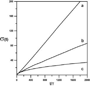
Figure 1: The standard deviation for the QKR as a function of time in units of $T$, with the parameters $\kappa_{1}=1$, $\kappa_{2}=-1$ and $p/q=1/3$. (a) $\alpha=0.2$ and $c=0.998$; (b) $\alpha=1$ and $c=0.772$; (c) $\alpha=2$ and $c=0.518$.

We have verified that the exponent $c$ has a dependence with the strength parameters $\kappa_{1}$and $\kappa_{2}$ and its range is always between $0.5$ and $1$, thus the sub-ballistic behavior is maintained. In Fig. 1 $\sigma(t)$ is plotted for several values of the parameter $\alpha$, displaying the qualitative differences between the periodic case $(\alpha\sim 0,$ $c\sim 1)$, the Lévy noise case $(0<\alpha<2$ and $0.5<c<1)$ and the Gaussian case $(\alpha\sim 2,$ $c\sim 0.5)$. The exponent $c$ is plotted in Fig. 2 as a function of $\alpha$ showing a clear dependence of $c$ with $\alpha$. We have also studied higher moments of order four and six, they all have smaller exponents than those obtained with a periodical sequence, thus the asymptotic behavior of these moments is consistent with the power-law behavior of the second moment.

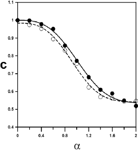
Figure 2: The exponent $c$ of the power law of the standard deviation as a function of the parameter $\alpha$. (a) The black dots correspond to the QKR with $\kappa_{1}=1$, $\kappa_{2}=-1$ and $p/q=1/3$, the full line is an adjustment. The parameters for the QKR are.; (b) The white dots correspond to the QW with $\theta_{1}=\pi/3$, $\theta_{2}=\pi/6$, the dashed line is an adjustment.

Quantum walk.-

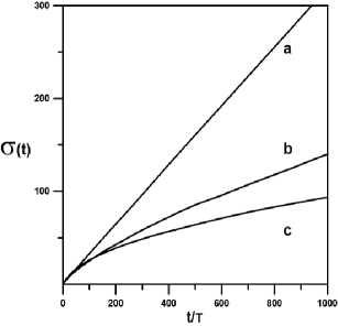
Figure 3: The standard deviation for the QW as a function of time in units of $T$ with the parameters $\theta_{1}=\pi/3$ and $\theta_{2}=\pi/6$. (a) $\alpha=0.2$ and $c=988$; (b) $\alpha=1$ and $c=0.71$; (c) $\alpha=2$ and $c=0.546$.

The standard QW corresponds to a one-dimensional evolution of a quantum system (the walker), in a direction which depends on an additional degree of freedom, the chirality, with two possible states: “left” $|L\rangle$ or “right” $|R\rangle$. The global Hilbert space of the system is the tensor product $H_{s}\otimes H_{c}$ where $H_{s}$ is the Hilbert space associated to the motion on the line and $H_{c}$ is the chirality Hilbert space. Let us call $T_{-}$ ($T_{+}$) the operators in $H_{s}$ that move the walker one site to the left (right), and $|L\rangle\langle L|$ and $|R\rangle\langle R|$ the chirality projector operators in $H_{c}$. We consider the unitary transformations

$$U(\theta)=\left\{T_{-}\otimes|L\rangle\langle L|+T_{+}\otimes|R\rangle\langle R|\right\}\circ\left\{I\otimes K(\theta)\right\},$$ (6)

where $K(\theta)=\sigma_{z}e^{-i\theta\sigma_{y}}$, $I$ is the identity operator in $H_{s}$, and $\sigma_{y}$ and $\sigma_{z}$ are Pauli matrices acting in $H_{c}$. The unitary operator $U(\theta)$ evolves the state in one time step, $|\Psi(t+1)\rangle=U(\theta)|\Psi(t)\rangle$. Here we are generalizing the QW to the case where different quantum coins are applied as in Ribeiro . As for the QKR, we combine two different step operators $U_{0}=U(\theta_{1})$ and $U_{1}=U(\theta_{2})$, with $\theta_{1}\neq\theta_{2}$, into a large sequence where we apply the same Lévy waiting time distribution. The wave function spreading is given by the exponent $c$ in $\sigma(t)=\sqrt{\sum_{i=0}^{\infty}i^{2}\left(\left|a_{i}(t)\right|^{2}+\left|b_{i}(t)\right|^{2}\right)}\sim t^{c}$. We take as the initial condition for the QW the position eigenstate $|0\rangle$, with chirality $(1,0)$ for the calculations of Fig. 3 and Fig. 2, and $(1,i)/\sqrt{2}$ for the calculations of Fig. 4. The standard deviation $\sigma(t)$ is numerically obtained for an ensemble of $1000$ trajectories for each value of the parameter $\alpha$ of the Lévy distribution. In Fig. 3 $\sigma(t)$ is plotted for different values of $\alpha$ and the sub-ballistic behavior is clearly shown. In Fig. 2 $c$ is plotted as a function of the parameter $\alpha$, here a functional dependence between them is evident. In Fig. 4 $c$ is plotted as a function of $\theta$, where $\theta=\theta_{1}=-\theta_{2}$This figure shows that the range of $c$ is always $\left[0.5,1\right]$, thus the sub-ballistic behavior is independent of the value of $\theta$ (except for the trivial cases $\theta=0$, $\theta=\pi/2$); additionally this figure is in concordance with Fig. $3$ in ref. Ribeiro These figures show qualitative similarities with the corresponding figures for the QKR, and point to the parallelism between the QW and the QKR in the secondary resonance regime. Again in this system, the moments of order four and six are consistent with the power-law behavior of the second moment.

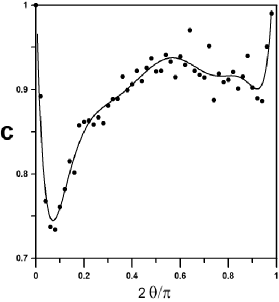
Figure 4: The exponent $c$ that characterizes de power law of the standard deviation for the QW as a function of the parameter $\theta$. The evolution is obtained with $\theta=\theta_{1}=-\theta_{2}$ in the interval $\left[0,\pi/2\right)$. The dots correspond to the calculation and the full line is a polynomial adjustment

Conclusion.- The quantum resonances and the DL of the QKR have been experimentally observed in samples of cold atoms interacting with a far-detuned standing wave of laser light expwave ; expqkr ; Ammann and in particular the secondary resonances have been recently observed by Kanem et al. Kanem . On the other hand several systems have been proposed as candidates to implement the QW model. These proposals include atoms trapped in optical lattices Dur , cavity quantum electrodynamics Sanders and nuclear magnetic resonance in solid substrates Du ; Berman . All these proposed implementations face the obstacle of decoherence due to environmental noise and imperfections. Thus the study of the behavior of these systems, subjected to different types of noise, is very important for the design and construction of future technologies. Here we proposed the study of the QKR and QW subjected to noisy pulses with a Lévy waiting time distribution. As Gaussian noise is a particular case of the Lévy noise, then our study is open to wider experimental situations. We prove that for QKR and QW the Lévy noise does not break completely the coherence in the dynamics but produces a sub-ballistic behavior in both systems, as an intermediate situation between the ballistic and the diffusive behavior. Then QKR and QW have essentially the same dynamical evolution and our results fortify the previously established parallelism between them alejo1 ; alejo2 ; alejo3 . More generally we can say that the dynamical evolution of the QKR and QW show certain patterns that seem to be common to a greater class of systems that are defined mainly by their symmetries and not by their microscopic details. The existence of an universality in the behavior of these systems suggests that one is allowed a larger flexibility in the choice of the physical systems to build quantum computers. It is important to highlight that the sub-ballistic behavior obtained in this paper for the QW and the QKR is essentially the same as that obtained for these systems when the perturbation follows a Fibonacci prescription Ribeiro ; alejo3 . The reason may lie in the fact that behind the Fibonacci prescription hides the lack of a typical scale in the sequence of the operators $U_{0}$ and $U_{1}$ which leads to a power law Henrik in the standard deviation, in the same way as for the Lévy noise.

We acknowledge the support from PEDECIBA and PDT S/C/OP/28/84.

References

- (1) F. M. Izrailev, Phys. Rep. 196, 299 (1990).
- (2) J. Kempe, Contemp. Phys. 44, 302 (2003); also in quant-ph/0303081
- (3) M. Nielssen and I. Chuang, Quantum Computation and Quantum Information, Cambridge University Press, 2000.
- (4) F.L. Moore, J.C. Robinson, C.F. Bharucha, B. Sundaram, and M.G. Raizen, Phys. Rev. Lett. 75, 4598 (1995)
- (5) J.F. Kanem, S. Maneshi, M. Partlow, M. Spanner and A. M. Steinberg in quant-ph/0604110.
- (6) Y. Aharonov, L. Davidovich and N. Zagury Phys. Rev. A 48, 1687 (1993).
- (7) S. Godoy and S. Fujita, J. Chem. Phys. 97, 5148 (1992).
- (8) A. Romanelli, A.C. Sicardi Schifino, R. Siri, G. Abal, A. Auyuanet and R. Donangelo. Physica A, 338, 395 (2004); also in quant-ph/0310171.
- (9) A. Romanelli, A. Auyuanet, R. Siri, G. Abal and R. Donangelo. Physica A, 352, 409 (2005); also in quant-ph/0408183.
- (10) A. Romanelli, A. Auyuanet, R. Siri and V. Micenmacher. Phys. Lett. A, 365, 200-203 (2007); also in quant-ph/0607146.
- (11) P. Ribeiro, P. Milman and R. Mosseri, Phys. Rev. Lett. 93, 190503 (2004).
- (12) G. Casati, G. Mantica and D.L. Shepelyansky Phys. Rev. E 63, 066217 (2001).
- (13) H. Schomerus and E. Lutz in quant-ph/0611162
- (14) P. Lévy, Theorie de l’Addition de Variables Aleatoires, Gauthier-Villiars, Paris (1937)
- (15) M. F. Shlesinger, G.M. Zaslavsky and J. Klafter, Nature 363, 31 (1993).
- (16) J. Klafter, M. F. Shlesinger, and G. Zumofen, Phys. Today 49 (2), 33 (1996).
- (17) G. M. Zaslavsky Phys. Today 52 (8), 39 (1999).
- (18) F.L. Moore, J.C. Robinson, C. Bharucha, P.E. Williams and M.G. Raizen, Phys. Rev. Lett. 73, 2974 (1994).
- (19) J.C. Robinson, C. Bharucha, F.L. Moore, R. Jahnke, G.A. Georgakis, Q. Niu, M.G. Raizen and B. Sundaram Phys. Rev. Lett. 74, 3963 (1995); J.C. Robinson, C.F. Bharucha, K.W. Madison, F.L. Moore, Bala Sundaram, S.R. Wilkinson and M.G. Raizen, Phys. Rev. Lett. 76, 3304 (1996).
- (20) H. Ammann, R. Gray, I. Shvarchuck and N. Christensen, Phys. Rev. Lett. 80, 4111 (1998).
- (21) W. Dür, R. Raussendorf, V.M. Kendon and H.J. Briegel, Phys. Rev. A 66, 052319 (2002); arXiv:quant-ph/0207137.
- (22) B.C. Sanders, S.D. Bartlett, B. Tregenna and P.L. Knight, Phys. Rev. A 67, 042305 (2003); arXiv:quant-ph/0207028.
- (23) J. Du, X. Xu, M. Shi, J. Wu, X. Zhou and R. Han, Phys. Rev. A 67, 042316 (2003).
- (24) G.P. Berman, D.I. Kamenev, R.B. Kassman, C. Pineda and V.I. Tsifrinovich, Int. J. Quant. Inf. 1, 51 (2003); arXiv:quant-ph/0212070
- (25) H. J. Jensen, Self-Organized Criticality, Cambridge University Press, 1998