Geodesics for Efficient Creation and Propagation of Order along Ising Spin Chains

Abstract

Experiments in coherent nuclear and electron magnetic resonance, and optical spectroscopy correspond to control of quantum mechanical ensembles, guiding them from initial to final target states by unitary transformations. The control inputs (pulse sequences) that accomplish these unitary transformations should take as little time as possible so as to minimize the effects of relaxation and decoherence and to optimize the sensitivity of the experiments. Here we give efficient syntheses of various unitary transformations on Ising spin chains of arbitrary length. The efficient realization of the unitary transformations presented here is obtained by computing geodesics on a sphere under a special metric. We show that contrary to the conventional belief, it is possible to propagate a spin order along an Ising spin chain with coupling strength $J$ (in units of Hz), significantly faster than $(2J)^{-1}$ per step. The methods presented here are expected to be useful for immediate and future applications involving control of spin dynamics in coherent spectroscopy and quantum information processing.

I Introduction

According to the postulates of quantum mechanics, the evolution of the state of a closed quantum system is unitary and is governed by the Schröedinger equation. This evolution of the state of a quantum system can be controlled by changing the Hamiltonian of the system. The control of quantum systems has important applications in physics and chemistry. In particular, the ability to steer the state of a quantum system (or an ensemble of quantum systems) from a given initial state to a desired target state forms the basis of spectroscopic techniques such as nuclear magnetic resonance (NMR) and electron spin resonance (ESR) spectroscopy Ernst ; electron and laser coherent control optics and quantum computing QC1 ; QC2 . Developing a specific set of control laws - pulse sequences- which produce a desired unitary evolution of the state has been a major thrust in NMR spectroscopy Ernst . For example, in the NMR spectroscopy of proteins Cavanagh , the transfer of coherence along spin chains is an essential step in a large number of key experiments. Spin chain topologies have also been proposed as architectures for quantum information processing kane ; yamamoto . In practice, the transfer time should be as short as possible, in order to reduce the loss due to relaxation or decoherence.

The time-optimal synthesis of unitary operators is now well understood for coupled two-spin systems navintoc ; Bennett ; Timo2spin ; General2spin ; yuan . This problem has also been recently studied in the context of linear three-spin topologies navingeodes ; navingeodes_exp ; navingeodes2 , where significant savings in the implementation time of trilinear Hamiltonians and synthesis of couplings between indirectly coupled qubits were demonstrated over conventional methods. In navingeodes ; navingeodes_exp ; navingeodes2 , it was shown that the time-optimal synthesis of indirect couplings and of trilinear Hamiltonians from linear Ising couplings can be reduced to the problem of computing singular geodesics. In this paper we extend these methods to linear Ising spin chains of size greater than $3$. In navin.chain , the problem of efficient propagation of spin coherences was studied. It was shown that by encoding the inital state of a spin into certain so called soliton operators, it is possible to propagate the unknown spin state through a spin chain at a rate of $(2J)^{-1}$ per step. In this paper, we extend these ideas to finding efficient ways to synthesize multiple-spin order and propagate coherences in linear Ising spin chains. Our methods are based on reducing the problem of efficient synthesis of the unitary propagator with the available Hamiltonians in minimum time to finding geodesics on a sphere under a suitable metric detailed subsequently. The main result of this paper is that contrary to common belief, it is possible to propagate a spin order along an Ising spin chain with coupling strength of $J$ (in units of Hz) between nearest neighbours, significantly faster than $(2J)^{-1}$ per step. We present explicit pulse sequences for advancing a spin order along an Ising spin at a rate $\sim\frac{\sqrt{2}-1}{J}$, which reduces the propagation time to $81\%$ of the best known methods.

Numerous approaches have been proposed and are currently used Cavanagh to transfer polarization or coherence through chains of coupled spins. Examples are pulse trains that create an effective ’XY’ Hamiltonian XYa ; XYb ; Advances which make it possible to propagate spin waves in such chains spinwave1 ; spinwave2 ; Brueschweiler . In order to achieve the maximum possible transfer amplitude, many other approaches have been developed, that rely either on a series of selective transfer steps between adjacent spins or on simple concatenations of two such selective transfer steps Cavanagh ; Advances . In our recent work, we showed by suitable encodings of the spin operators it is possible to transfer the unknown state of a spin at the rate of $\frac{1}{2J}$ time units per step through the spin chain navingeodes2 . Subsequently, the problem has been studied in other contexts, see jones1 ; twamley and references in there. We show that methods presented here are significantly shorter than these state of the art techniques. Furthermore, the transfer mechanisms that result from the methods presented have a clear geometric interpretation.

II Theory

We consider a linear chain of $n$ spins, placed in a static external magnetic field in the $z$ direction, with equal Ising type couplings between next neighborsIsing1925 ; Caspers . In a suitably chosen (multiple) rotating frame, which rotates with each spin at its resonant frequency, the free evolution of the spin system is given by the coupling Hamiltonian

$$H_{c}=2\pi J\sum_{m=1}^{n-1}I_{mz}I_{(m+1)z}.$$

We assume that the Larmor frequency of the spins are well separated compared to the coupling constant $J$, so that we can selectively rotate each spin at a rate much faster than the evolution of the couplings. The goal of the pulse designer is to make an appropriate choice of the control variables like the amplitude and phase of the external RF field to effect a net desired unitary evolution.

We first consider the problem of synthesizing a unitary $U$, which efficiently transfers a single spin coherence represented by the initial operator $I_{1x}$ to a multiple spin order represented by the operator $2^{n-1}\prod_{m=1}^{n}I_{mz}$. This transfer is routinely performed in multidimensional high resolution NMR experiments Cavanagh . The techniques developed in solving this problem time optimally will be used subsequently for other key transfers.

The conventional strategy for achieving this transfer is achieved through the following stages

$$\begin{aligned} &I_{1x}\stackrel{{\scriptstyle H_{c}}}{{\rightarrow}}2I_{1y}I_{2z}\stackrel{{\scriptstyle I_{2y}}}{{\rightarrow}}2I_{1y}I_{2x}\stackrel{{\scriptstyle H_{c}}}{{\rightarrow}}4I_{1y}I_{2y}I_{3z}\\ &\stackrel{{\scriptstyle I_{3y}}}{{\rightarrow}}4I_{1y}I_{2y}I_{3x}\rightarrow\cdots\rightarrow 2^{n-1}(\prod_{m=1}^{n-1}I_{my})I_{nz}\end{aligned}$$ (1)

In the first stage of the transfer, operator $I_{1x}$ evolves to $2I_{1y}I_{2z}$ under the natural coupling Hamiltonian $H_{c}$ in $\frac{1}{2J}$ units of time. This operator is then rotated to $2I_{1y}I_{2x}$ by applying a hard $(\frac{\pi}{2})_{y}$ pulse on the second spin, which evolves to $4I_{1y}I_{2y}I_{3z}$ under the natural coupling, followed by a hard $(\frac{\pi}{2})_{y}$ pulse on spin $3$ and so on. The final state $2^{n-1}(\prod_{m=1}^{n-1}I_{my})I_{nz}$ prepared in this manner is locally equivalent to $2^{n-1}\prod_{m=1}^{n}I_{mz}$. The whole transfer involves $n-1$ evolution steps under the natural Hamiltonian, each taking $\frac{1}{2J}$ units of time, resulting in a total time of $\frac{n-1}{2J}$. We now formulate the problem of this transfer as a problem of optimal control and derive time efficient strategies for achieving this transfer.

Figure 1: The figure depicts the conventional pulse sequence for the creation of multiple spin order as in Equation (1). The spins are sequentially irradiated with hard $(\frac{\pi}{2})_{y}$ pulses with a period of $\tau=\frac{1}{2J}$ between them for the evolution of natural coupling.

III The Optimal Control Problem

To simplify notation, we introduce the following symbols for the expectation values of operators that play a key part in the transfer.

$$\begin{aligned} &x_{1}=<I_{1x}>\\ &x_{2}=<2I_{1y}I_{2z}>\\ &x_{3}=<2I_{1y}I_{2x}>\\ &x_{4}=<4I_{1y}I_{2y}I_{3z}>\\ &\vdots\\ &x_{2n-3}=<2^{n-1}I_{1y}I_{2y}I_{3y}\cdots I_{(n-1)x}>\\ &x_{2n-2}=<2^{n-1}I_{1y}I_{2y}I_{3y}\cdots I_{(n-1)y}I_{nz}>\end{aligned}$$ (2)

Let $X=(x_{1},x_{2},x_{3},\dots,x_{2n})^{T}$. The evolution of the system is given by

$$\frac{dX}{dt}=\pi J\left(\begin{array}[]{cccccccc}0&-1&0&0&0&0&\cdots\\ 1&0&-u_{1}&0&0&0&\cdots\\ 0&u_{1}&0&-1&0&0&\cdots\\ 0&0&1&0&-u_{2}&0&\cdots\\ 0&0&0&u_{2}&0&-1&\cdots\\ 0&0&0&0&1&0&\cdots\\ \vdots&\vdots&\vdots&\vdots&\vdots&\vdots&\vdots&\vdots\par\end{array}\right)X$$ (3)

where $u_{k}$ are the control parameters representing the amplitude of the $y$ pulse on spin $k+1$. The problem now is to find the optimal $u_{k}(t)$, steering the system from $(1,0,0,\cdots,0)$ to $(0,0,\cdots,0,1)$ in the minimum time.

In this picture, the conventional transfer method is described as setting all $u_{k}=0$ for $\frac{1}{2J}$ units of time, then transfer $x_{1}=1\rightarrow x_{2}=1$. Now using the control $u$, we rotate $x_{2}=1$ to $x_{3}=1$ in arbitrary small time as control can be performed arbitrarily fast (compared to the evolution of couplings). Now we set $u_{k}=0$ again, evolve $\frac{1}{2J}$ units of time under natural Hamiltonian, transfer $x_{3}=1$ to $x_{4}=1$ and so on. This way the total time for the transfer is $\frac{(n-1)}{2J}$.

We now show how significantly shorter transfer times are achievable, if we relax the constraint that the selective rotations on a given spin are only hard pulses. We show that if we let the selective operations be carried out by soft shaped pulses, along with evolution of the coupling Hamiltonian, then we can achieve significantly shorter transfer time. The analytical pulse shapes can be computed by formulating the problem as computation of geodesics on a sphere under a special metric. We divide the total transfer into transfer steps. We first transfer $x_{1}=1$ to $x_{3}=x_{4}=\frac{1}{\sqrt{2}}$, then transfer $x_{3}=x_{4}=\frac{1}{\sqrt{2}}$ to $x_{5}=x_{6}=\frac{1}{\sqrt{2}}$ and so on and finally at the last transfer $x_{2n-3}=x_{2n-2}=\frac{1}{\sqrt{2}}$ to $x_{2n}=1$. The first step is described by the following equation. The subsequent steps can also be understood by relating them to the following equation (we suppress the factor of $\pi J$ in the front of the equation).

$$\frac{d}{dt}\left(\begin{array}[]{c}x_{1}\\ x_{2}\\ x_{3}\\ x_{4}\end{array}\right)=\left(\begin{array}[]{cccc}0&-1&0&0\\ 1&0&-u&0\\ 0&u&0&-1\\ 0&0&1&0\par\end{array}\right)\left(\begin{array}[]{c}x_{1}\\ x_{2}\\ x_{3}\\ x_{4}\end{array}\right),$$ (4)

We make the following change of variables. Let

$$r_{1}=x_{1},r_{2}=\sqrt{x_{2}^{2}+x_{3}^{2}},r_{3}=x_{4},\tan\theta=\frac{x_{3}}{x_{2}}$$

as depicted in the following picture.

Figure 2: The figure depicts the control angle $\theta$

Using $u$, we can control the angle $\theta$, so we can think of $\theta$ as a control variable. The equation for the evolution of $r_{i}$ are

$$\frac{d}{dt}\left(\begin{array}[]{c}r_{1}\\ r_{2}\\ r_{3}\\ \end{array}\right)=A\left(\begin{array}[]{c}r_{1}\\ r_{2}\\ r_{3}\\ \end{array}\right),$$ (5)

where

$$A=\left(\begin{array}[]{ccc}0&-\cos\theta(t)&0\\ \cos\theta(t)&0&-\sin\theta(t)\\ 0&\sin\theta(t)&0\\ \end{array}\right).$$

We now need to find $\theta(t)$ for steering the system from $(1,0,0)$ to $(0,\frac{1}{\sqrt{2}},\frac{1}{\sqrt{2}})$ in the minimum time.

We now show that this is equivalent to find the geodesic on the sphere from $(1,0,0)$ to $(0,\frac{1}{\sqrt{2}},\frac{1}{\sqrt{2}})$ under the metric $g=\frac{dr_{1}^{2}+dr_{3}^{2}}{r_{2}^{2}}$ navingeodes2 .

The time of transfer $\tau$ can be written as $\int_{0}^{\tau}\sqrt{\sin^{2}\theta(t)+\cos^{2}\theta(t)}\ dt$. Substituting for $\sin\theta(t)$ and $\cos\theta(t)$ from (5), this reduces to

$$\int\underbrace{\sqrt{\frac{(\dot{r}_{1})^{2}+(\dot{r}_{3})^{2}}{r_{2}^{2}}}}_{L}dt.$$

Thus minimizing $\tau$ amounts to computing the geodesic under the metric

$$g={\frac{dr_{1}^{2}+dr_{3}^{2}}{r_{2}^{2}}}.$$

The Euler-Lagrange equations for the geodesic take the form $\frac{d}{dt}(\frac{\partial L}{\partial\dot{r}_{1}})=\frac{\partial L}{\partial r_{1}}$ and $\frac{d}{dt}(\frac{\partial L}{\partial\dot{r}_{3}})=\frac{\partial L}{\partial r_{3}}$. Note, $r_{2}^{2}=1-r_{1}^{2}-r_{3}^{2}$ and along the geodesic, $L$ is constant. We get

$$\frac{d}{dt}\frac{\dot{r}_{1}}{r_{2}^{2}}=L^{2}\frac{r_{1}}{r_{2}^{2}};\ \ \frac{d}{dt}\frac{\dot{r}_{3}}{r_{2}^{2}}=L^{2}\frac{r_{3}}{r_{2}^{2}}$$ (6)

which implies that

$$\frac{d}{dt}\frac{\dot{r}_{1}r_{3}-\dot{r}_{3}r_{1}}{r_{2}^{2}}=0$$

Let $f=\frac{\dot{r}_{3}r_{1}-\dot{r}_{1}r_{3}}{r_{2}^{2}}$, then $f$ is constant along the optimal trajectory. For $f$ to be finite, we need $\sin\theta(0)=0$, i.e., $\theta(0)=0$. From Eq. 6, we get

$$\frac{d}{dt}(\frac{\dot{r}_{1}}{r_{2}})=f\frac{\dot{r}_{3}}{r_{2}}$$ (7)

Substitute $\frac{\dot{r}_{1}}{r_{2}}=-\cos\theta(t)$,$\frac{\dot{r}_{3}}{r_{2}}=\sin\theta(t)$, gives

$$\frac{d}{dt}(-\cos\theta(t))=f\sin\theta(t),$$

so $\dot{\theta}=f$,

$$\theta(t)=ft+\varphi$$

Since $\theta(0)=0$ we get $\varphi=0$. We can now simply search numerically for the constant $f$ and it turns out that for the transfer from $(1,0,0)$ to $(0,\frac{1}{\sqrt{2}},\frac{1}{\sqrt{2}})$, the optimal $f$ (in units of $\pi J$) and the minimum time $\tau_{1}$ (in units of $\frac{1}{\pi J}$) are

$$f=0.542,\ \ \ \tau_{1}=1.94\sim\frac{3\pi(\sqrt{2}-1)}{2}$$ (8)

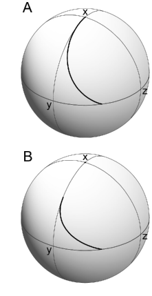
Figure 3: The curve in Fig. A, depicts the shortest path connecting the north pole $(1,0,0)$ to a point $(0,\frac{1}{\sqrt{2}},\frac{1}{\sqrt{2}})$, under the metric $g$. The curve in Fig. B, depicts the shortest path connecting $(\frac{1}{\sqrt{2}},\frac{1}{\sqrt{2}},0)$ to a point $(0,\frac{1}{\sqrt{2}},\frac{1}{\sqrt{2}})$, under the metric $g$.

Now differentiating the expression, $\frac{x_{3}}{x_{2}}(t)=\tan(\theta(t))$ gives that $u(t)$ in is constant with a value $u=1.084$. The subsequent transfer steps, whereby $(x_{k},x_{k+1})=(\frac{1}{\sqrt{2}},\frac{1}{\sqrt{2}})$ is transferred to $(x_{k+2},x_{k+3})=(\frac{1}{\sqrt{2}},\frac{1}{\sqrt{2}})$, are described by the same equation of the type as (4), except we now want to transfer from initial state $(\frac{1}{\sqrt{2}},\frac{1}{\sqrt{2}},0,0)$ to final state $(0,0,\frac{1}{\sqrt{2}},\frac{1}{\sqrt{2}})$ for the intermediate steps and finally from $(\frac{1}{\sqrt{2}},\frac{1}{\sqrt{2}},0,0)$ to $(0,0,0,1)$ for the last step. For the intermediate steps, using the same method as before, we get $f$ (in the units of $\pi J$) and the minimum time $\tau_{2}$ (in units of $(\pi J)^{-1}$) as

$$f=1.2377,\tau_{2}=1.2692\sim(\sqrt{2}-1)\pi.$$ (9)

The optimal $u(t)$ in Eq. (4) for this transfer is shown in Fig. 4.

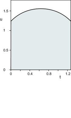
Figure 4: Fig. shows the optimal $u(t)$ in Eq. (4) for the transfer $(\frac{1}{\sqrt{2}},\frac{1}{\sqrt{2}},0,0)$ to $(0,0,\frac{1}{\sqrt{2}},\frac{1}{\sqrt{2}})$. The time is in the units of $(\pi J)^{-1}$.

.

The optimal transfer for the last step takes the same time as in (8). The total time (in units of $(\pi J)^{-1}$ ) is

$$\sim\pi((n-1)(\sqrt{2}-1)),$$

which is approximately $81\%$ of the conventional method described earlier.

Figure 5: The figure depicts the new pulse sequence for the creation of multiple spin order. The spins $I_{3}$ to $I_{n-2}$ are sequentially irradiated with shaped pulses as in Fig. 4, with pulse duration of $\tau_{2}$. The couplings evolve during the pulse duration and there is no delay between the sequential pulses. The initial rectangular pulse of duration $\tau_{1}$ on spin 2, creates the state $(x_{3},x_{4})=(\frac{1}{\sqrt{2}},\frac{1}{\sqrt{2}})$ in (2). The final rectangular pulse of duration $\tau_{1}$ on spin $I_{n-1}$, creates the desired spin order.

We now use these methods for finding efficient ways to propagate coherences along Ising spin-chains.

III.1 Efficient Transfer of Coherence

Consider the transfer of coherence

$$I_{1x}\rightarrow I_{nx},$$

between the spins $1$ and $n$.

The fastest conventional method for achieving this transfer is based on the concatenated INEPT transfer concatenation , whereby bilinear operators $2I_{kx}I_{(k+1)z}$ are propagated through the spin chain using the following steps:

$$2I_{kx}I_{(k+1)z}\stackrel{{\scriptstyle(H_{1})_{\frac{\pi}{2}}}}{{\rightarrow}}-2I_{kz}I_{(k+1)x}\stackrel{{\scriptstyle(H_{c})_{\frac{\pi}{2}}}}{{\rightarrow}}2I_{(k+1)x}I_{(k+2)z}.$$ (10)

The control Hamiltonian $H_{1}=(I_{ky}+I_{(k+1)y})$ evolves for a time corresponding to $\frac{\pi}{2}$ rotation, (this step takes arbitrarily small time), followed by evolution of the coupling Hamiltonian $H_{c}$ for $\frac{1}{2J}$ units of time. Under this transfer strategy, bilinear operators are propagated through the spin chain at a propagation speed of $\frac{1}{2J}$. We now show how the propagation rate of coherences through the chain can be enhanced by preparing suitable spin states and efficient transfer of these states using methods described before. Using these ideas, it becomes possible to transfer the operators one step along the chain in only $\frac{\sqrt{2}-1}{J}$ units of time.

$\Lambda_{1k}$	$4I_{kz}I_{(k+1)y}I_{(k+2)x}$
$\Lambda_{2k}$	$8I_{kz}I_{(k+1)y}I_{(k+2)y}I_{(k+3)z}$
$\Lambda_{3k}$	$2I_{(k+1)x}I_{(k+2)x}$
$\Lambda_{4k}$	$4I_{(k+1)x}I_{(k+2)y}I_{(k+3)z}$
$D_{1k}$	$8I_{kz}I_{(k+1)y}I_{(k+2)y}I_{(k+3)x}$
$D_{2k}$	$16I_{kz}I_{(k+1)y}I_{(k+2)y}I_{(k+3)y}I_{(k+4)z}$
$D_{3k}$	$4I_{(k+1)x}I_{(k+2)y}I_{(k+3)x}$
$D_{4k}$	$8I_{(k+1)x}I_{(k+2)y}I_{(k+3)y}I_{(k+4)z}$

Table 1: Relevant operators for transfer of spin order.

Consider the operator

$$\Lambda_{k} = \frac{1}{2}(\Lambda_{1k}+\Lambda_{2k}+\Lambda_{3k}+\Lambda_{4k}),$$ (11)

where various operators in the equation are displayed in Table I. By application of the Hamiltonian $H=H_{c}+u(t)H_{2}$, the operator $\Lambda_{k}$ is advanced one step in the spin chain,

$$\Lambda_{k}\stackrel{{\scriptstyle H}}{{\longrightarrow}}\Lambda_{k+1},$$

where $H_{2}=\pi J(I_{(k+1)y}+I_{(k+3)y})$ and $u(t)$ is the optimally shaped pulse that transfers $(\frac{1}{\sqrt{2}},\frac{1}{\sqrt{2}},0,0)$ to $(0,0,\frac{1}{\sqrt{2}},\frac{1}{\sqrt{2}})$ in equation (4) in the minimum time. The time of this transfer is $\tau_{2}\sim\frac{(\sqrt{2}-1)}{J}$ and it advances the spin operators one step in the spin chain. This is best understood by splitting the Hamiltonian $H$ into two commuting Hamiltonians $H_{a}=\pi J(2I_{(k+2)z}I_{(k+3)z}+2I_{(k+3)z}I_{(k+4)z}+u(t)I_{(k+3)y})$ and $H_{b}=\pi J(2I_{kz}I_{(k+1)z}+2I_{(k+1)z}I_{(k+2)z}+u(t)I_{(k+1)y})$, whose action can be analyzed separately. We identify $(\langle\Lambda_{1k}\rangle,\langle\Lambda_{2k}\rangle,\langle D_{1k}\rangle,\langle D_{2k}\rangle)$ and $(\langle\Lambda_{3k}\rangle,\langle\Lambda_{4k}\rangle,\langle D_{3k}\rangle,\langle D_{4k}\rangle)$ with $(x_{1},x_{2},x_{3},x_{4})$.

Under the action of the Hamiltonian $H_{a}$, the evolution of the operators $(x_{1},x_{2},x_{3},x_{4})$ is exactly identical to the one in equation (4). If $u(t)$ is chosen optimally, as described, in Fig. 4, we transfer the state $(\langle\Lambda_{1k}\rangle,\langle\Lambda_{2k}\rangle,\langle D_{1k}\rangle,\langle D_{2k}\rangle)=(\frac{1}{2},\frac{1}{2},0,0)$ to $(0,0,\frac{1}{2},\frac{1}{2})$. Similarly $(\langle\Lambda_{3k}\rangle,\langle\Lambda_{4k}\rangle,\langle D_{3k}\rangle,\langle D_{4k}\rangle)=(\frac{1}{2},\frac{1}{2},0,0)$ is transferred to $(0,0,\frac{1}{2},\frac{1}{2})$. So under $H_{a}$, $\Lambda_{k}$ is transferred to $\frac{1}{2}(D_{1k}+D_{2k}+D_{3k}+D_{4k})$.

Similar analysis shows that under the action of $H_{b}$, we transfer $(\langle D_{1k}\rangle,\langle D_{2k}\rangle,\langle D_{3k}\rangle,\langle D_{4k}\rangle)=\frac{1}{2}(1,1,1,1)$ to $(\langle\Lambda_{1(k+1)}\rangle,\langle\Lambda_{2(k+1)}\rangle,\langle\Lambda_{3(k+1)}\rangle,\langle\Lambda_{4(k+1)}\rangle)=\frac{1}{2}(1,1,1,1)$, which is the desired operator $\Lambda_{k+1}$.

Creation of the operator $\Lambda_{1}$ from the operator $I_{1x}$ can also be achieved in many ways. Here we present one such preparation, (which is not necessarily time optimal). Similarly, the final operator $\Lambda_{n-3}$ can be collapsed on to the final state $I_{nx}$ using steps as before.

$$\begin{aligned} &I_{1x}\stackrel{{\scriptstyle(H_{c})_{\frac{\pi}{2}}}}{{\rightarrow}}2I_{1y}I_{2z}\stackrel{{\scriptstyle(I_{2y})_{\frac{\pi}{2}}}}{{\rightarrow}}2I_{1y}I_{2x}\stackrel{{\scriptstyle(H_{c})_{\frac{\pi}{2}}}}{{\rightarrow}}4I_{1y}I_{2y}I_{3z}\\ &\stackrel{{\scriptstyle(I_{3y})_{\frac{\pi}{2}}}}{{\rightarrow}}4I_{1y}I_{2y}I_{3x}\stackrel{{\scriptstyle(H_{c})_{\frac{\pi}{4}}}}{{\rightarrow}}\frac{1}{\sqrt{2}}(4I_{1y}I_{2y}I_{3x}+8I_{1y}I_{2y}I_{3y}I_{4z}).\end{aligned}$$ (12)

Now by applying a $(\frac{\pi}{2})_{x}$ pulse on the first spin, we will get a superposition of $4I_{1z}I_{2y}I_{3x}$ and $8I_{1z}I_{2y}I_{3y}I_{4z}$. Now, letting the natural coupling $H_{c}$ evolve for another $\frac{\pi}{4}$ rotation period with spin $4$ is decoupled, followed by a $(\pi)_{y}$ pulse on spin 2, we will generate the operator $\Lambda_{1}$.

We now show how these ideas can be generalized for transferring the unknown state of a spin $1$ to spin $n$. All we need to show is that we can simultaneously transfer $I_{1x}\rightarrow I_{nx}$ and $I_{1y}\rightarrow I_{ny}$, and this ensures that $I_{1z}$ is transferred to $I_{nz}$. Furthermore, this ensures that an arbitrary unknown state of spin $1$, ($aI_{1z}+bI_{1x}+cI_{1y}$), is transferred to the final state ($aI_{nz}+bI_{nx}+cI_{ny}$). Consider the pair of operators $(\Lambda_{k},\Lambda_{k+2})$, where $\Lambda_{k}$ is defined in Eq.(11). Then observe,

$$(\Lambda_{k},\Lambda_{k+2})\stackrel{{\scriptstyle(H)}}{{\longrightarrow}}(\Lambda_{k+1},\Lambda_{k+3}),$$

where $H=H_{c}+u(t)\pi J(I_{(k+1)y}+I_{(k+3)y}+I_{(k+5)y})$ and $u(t)$ is the same optimal pulse shape as in Eq.(9) and it takes $\frac{\sqrt{2}-1}{J}$ units of time to advance the pair $(\Lambda_{k},\Lambda_{k+2})$, one step in the spin chain. We can now encode the operators $(I_{1y},I_{1x})$ via operators $(\Lambda_{1},\Lambda_{3})$ and transport it along the chain at a rate of $\frac{\sqrt{2}-1}{J}$ units of time per step. The encoding can be achieved by the following steps: first applying a $(\frac{\pi}{2})_{-x}$ pulse on the first spin, transfer $I_{1y}$ to $-I_{1z}$, then follow the steps in the last paragraph applying the pulses transferring $I_{1x}$ to $\Lambda_{1}$, these pulses will also transfer $-I_{1z}$ to $\frac{1}{\sqrt{2}}(I_{1y}+2I_{1x}I_{2z})$. We then apply the pulses transferring

$$\Lambda_{1}\stackrel{{\scriptstyle(H_{1})}}{{\longrightarrow}}\Lambda_{2}\stackrel{{\scriptstyle(H_{2})}}{{\longrightarrow}}\Lambda_{3},$$

where $H_{1}=H_{c}+u(t)\pi J(I_{2y}+I_{4y}),H_{2}=H_{c}+u(t)\pi J(I_{3y}+I_{5y})$ and $u(t)$ is the optimally shaped pulse that transfers $(\frac{1}{\sqrt{2}},\frac{1}{\sqrt{2}},0,0)$ to $(0,0,\frac{1}{\sqrt{2}},\frac{1}{\sqrt{2}})$ in equation (5) in the minimum time. These pulses will transfer $\frac{1}{\sqrt{2}}(I_{1y}+2I_{1x}I_{2z})$ to

$$\begin{aligned} &\frac{1}{\sqrt{2}}(I_{1y}+2I_{1x}I_{2z})\stackrel{{\scriptstyle(H_{1})}}{{\longrightarrow}}\frac{1}{\sqrt{2}}(2I_{1x}I_{2x}+4I_{1x}I_{2y}I_{3z})\\ &\stackrel{{\scriptstyle(H_{2})}}{{\longrightarrow}}\frac{1}{\sqrt{2}}(4I_{1x}I_{2y}I_{3x}+8I_{1x}I_{2y}I_{3y}I_{4z})\end{aligned}$$ (13)

then by applying a $(\frac{\pi}{2})_{-y}$ pulse on the first spin, we will get a superposition of $4I_{1z}I_{2y}I_{3x}$ and $8I_{1z}I_{2y}I_{3y}I_{4z}$ and let the natural coupling $H_{c}$, evolve for another $\frac{\pi}{4}$ rotation period with spin $4$ and $6$ decoupled, followed by a $(\pi)_{y}$ on spin 2, we will generate the operator $\Lambda_{1}$. Thus, we have succeeded in encoding $(I_{1y},I_{1x})$ in $(\Lambda_{1},\Lambda_{3})$. Compared to the recently developed methods, navin.chain that transport the two operators $(I_{1x},I_{1y})$ at a rate of $\frac{1}{2J}$ per step in the spin chain, the time taken by the proposed methods is about $81\%$ of these recently developed techniques.

IV Conclusion

In this article, we studied the problem of time optimal creation of multiple quantum coherences and transfer of coherences along linear Ising spin chains. We showed that by suitably encoding the initial state of the spin in certain operators, it is possible to propagate these operators along the spin chain at a rate $\sim\frac{\sqrt{2}-1}{J}$, which is significantly faster than the conventional belief that it takes $\frac{1}{2J}$ to advance spin operators in a spin chain. The methods developed in this paper may find applications in other problems of optimal control of coupled spin dynamics

References

• (1) R. R. Ernst, G. Bodenhausen, A. Wokaun, “Principles of Nuclear Magnetic Resonance in One and Two Dimensions”, Clarendon Press, Oxford (1987).
• (2) A. Schweiger, in Modern Pulsed and Continuous Wave Electron Spin Resonance, M.K. Bowman, Ed. (Wiley, London, 1990), pp 43-118.
• (3) W. S. Warren, H. Rabitz, M. Dahleh, Science 259, 1581 (1993).
• (4) N. A. Gershenfeld and I. L. Chuang, Science 275, 350 (1997).
• (5) D. G. Cory, A. Fahmy, T. Havel, Proc. Natl. Acad. Sci. USA 94, 1634 (1997).
• (6) J. Cavanagh, W. J. Fairbrother, A. G. Palmer, N. J. Skelton, Protein NMR Spectroscopy: Principles and Practice, (Academic Press, San Diego, 1996.)
• (7) B.E. Kane, Nature 393, 133 (1998).
• (8) F. Yamaguchi, Y. Yamamoto, Appl. Phys. A 68 (1999).
• (9) John B. Baillieul, PH.D Thesis.
• (10) N.Khaneja, R.Brockett and S.J.Glaser, Phys. Rev. A 63, 032308(2001).
• (11) C.H.Bennett, J.I.Cirac, M.S.Leifer, D.W.Leung, N.Linden, S.Popescu and G.Vidal, Phys. Rev. A 66, 012305(2002).
• (12) T. O. Reiss, N. Khaneja, S. J. Glaser, J. Magn. Reson., 154, 192-195 (2002).
• (13) N. Khaneja, F. Kramer, S. J. Glaser, J. Magn. Reson. 173, 116-124 (2005).
• (14) H. Yuan and N. Khaneja, Phys. Rev. A 72 040301(R) (2005).
• (15) N.Khaneja, S.J. Glaser and R.W. Brockett, Phys. Rev. A, 65, 032301(2002).
• (16) N. Khaneja, S. J. Glaser, ”Efficient transfer of coherence through Ising Spin chains”, Phys. Rev. A, 66, 060301(R) (2002).
• (17) T. O. Reiss, N. Khaneja, S. J. Glaser, J. Magn. Reson., 165, 95-101 (2003).
• (18) N. Khaneja, B. Heitmann, A. Spoerl, H. Yuan, T. Herbrueggen and S.J. Glaser, ”Shortest paths for efficient control of indirectly coupled qubits”, Phys. Rev. A, 75, 012322(2007) .
• (19) E. H. Lieb, T. Schultz, D. C. Mattis, Ann. Phys. (Paris) 16, 407 (1961).
• (20) H. M. Pastawski, G. Usaj, P. R. Levstein, Chem. Phys. Lett. 261, 329 (1996).
• (21) S. J. Glaser, J. J. Quant, in Advances in Magnetic and Optical Resonance, W. S. Warren, Ed. (Academic Press, San Diego, 1996), Vol. 19, pp. 59.
• (22) R. M. White, Quantum Theory of Magnetism (Springer, Berlin, 1983).
• (23) D. C. Mattis, The Theory of Magnetism I, Statistics and Dynamics (Springer, Berlin, 1988).
• (24) Z. L. Mádi, B. Brutscher, T. Schulte-Herbrüggen, R. Brüschweiler, R. R. Ernst, Chem. Phys. Lett. 268, 300 (1997).
• (25) E. Ising, Z. Physik 31, 253 (1925).
• (26) W. J. Caspers, Spin Systems (World Scientific, London, 1989).
• (27) J. Fitzsimons, L. Xiao, S. C. Benjamin, J. A. Jones, quant-ph/0606188 (2006).
• (28) J. Fitzsimons, J. Twamley, quant-ph/0601120 (2006).
• (29) T. Schulte-Herbrüggen, O.W. Sørensen, Concepts Magn. Reson. 12 389 (2000).
• (30) D. P. Weitekamp, J. R. Garbow, A. Pines, J. Chem. Phys. 77, 2870 (1982).
• (31) P. Caravatti, L. Braunschweiler, R. R. Ernst, Chem. Phys. Lett. 100, 305 (1983).
• (32) A. Majumdar, E. P. Zuiderweg, J. Magn. Reson. A 11 3, 19 (1995).