Detection of Crab Giant Pulses Using the Mileura Widefield Array Low Frequency Demonstrator Field Prototype System

Abstract

We report on the detection of giant pulses from the Crab Nebula pulsar at a frequency of 200 MHz using the field deployment system designed for the Mileura Widefield Array’s Low Frequency Demonstrator (MWA-LFD). Our observations are among the first high-quality detections at such low frequencies. The measured pulse shapes are deconvolved for interstellar pulse broadening, yielding a pulse-broadening time of 670$\pm$100 $\mu$s, and the implied strength of scattering (scattering measure) is the lowest that is estimated towards the Crab nebula from observations made so far. The sensitivity of the system is largely dictated by the sky background, and our simple equipment is capable of detecting pulses that are brighter than $\sim$9 kJy in amplitude. The brightest giant pulse detected in our data has a peak amplitude of $\sim$50 kJy, and the implied brightness temperature is $10^{31.6}$ K. We discuss the giant pulse detection prospects with the full MWA-LFD system. With a sensitivity over two orders of magnitude larger than the prototype equipment, the full system will be capable of detecting such bright giant pulses out to a wide range of Galactic distances; from $\sim$8 to $\sim$30 kpc depending on the frequency. The MWA-LFD will thus be a highly promising instrument for the studies of giant pulses and other fast radio transients at low frequencies.

1 Introduction

Giant pulses from the Crab Nebula pulsar have been known since the early days of pulsar observations (Staelin & Reifenstein 1968; Argyle & Gower 1972). These sporadic, large-amplitude bursts can exceed mean pulse energies by factors as large as $10^{4}$ (Lundgren et al., 1995), and they remain as an intriguing phenomenon for theories of the pulsar emission mechanism to explain. Their short durations also allow them to serve as sensitive probes of the nebula and the interstellar medium. Much has been learnt from observations so far, and it is fairly well established that: (i) the fluctuations in their amplitudes are associated with changes in the coherence of the radio emission (Lundgren et al., 1995), (ii) the emission is broadband – extending over several hundreds of MHz (Sallmen et al., 1999; Popov et al., 2006), and (iii) they are superpositions of extremely narrow nanosecond-duration structures (Hankins et al., 2003). The Crab giant pulses have some of the largest implied brightness temperatures of known astrophysical sources, and are known to reach $10^{32}$ K at microsecond time resolutions (Cordes et al., 2004), and even higher ($10^{37}$ K) at nanosecond resolutions (Hankins et al., 2003).

Although the Crab pulsar was originally discovered at a low radio frequency of 111 MHz (Staelin & Reifenstein, 1968) through detection of its giant pulses, the bulk of the observational studies of it over the past three decades has focused primarily at higher frequencies (e.g. Moffett & Hankins, 1996; Cordes et al., 2004). This is partly due to limitations imposed by the dispersive and scattering effects in the interstellar medium (ISM) that degrade the signal strength at low frequencies. A more significant reason perhaps is that most existing large instruments are optimised for best performance above 300 MHz. For single dishes this has been driven by a quest for sensitivity, and for interferometers by resolution and sensitivity, and also the need to avoid the problems due to ionospheric distortion of astronomical signal at low frequencies. The recent enormous increase in affordability of computing and the impressive advances in the capabilities of digital hardware have brought the computational needs of low frequency radio imaging within reach. This has led to a resurgence in the interest in low frequency astronomy and a number of instruments like the Mileura Widefield Array Low Frequency Demonstrator (MWA-LFD) in Western Australia, Low Frequency Array (LOFAR) in the Netherlands and Long Wavelength Array (LWA) in South-west US are currently in varying stages of design, development and deployment. The ever growing problem of man made radio frequency interference (RFI) continues to remain a major concern however, especially in densely populated parts of the world.

Despite the paucity of low-frequency studies of the Crab, a wealth of information can be gleaned from such studies. As such pulsar radio emission is strongly frequency dependent, with most intrinsic and extrinsic effects becoming more pronounced at lower radio frequencies. In particular, the Crab pulsar is well known for its highly peculiar and complex frequency evolution of its pulse morphology and structure (Cordes et al., 2004; Moffett & Hankins, 1996). Therefore it would be interesting to examine how the properties of pulse emission evolve at low radio frequencies. Further, the scattering and dispersion effects also become more prominent with decreasing observing frequency, and are best studied at low frequencies.

The MWA-LFD is a promising instrument with capabilities that will complement those of existing large telescopes, particularly the frequency coverage. Given its high sensitivity, multi-beaming and wide field-of-view capabilities, this instrument promises excellent prospects for pulsar and transient science. In this paper, we report on successful detection of the Crab giant pulses at 200 MHz using the prototype system that was built for its early deployment activities. Although the Crab pulsar was detected earlier at a nearby frequency (196.5 MHz) via its average emission (Rankin et al., 1970), our observations mark the first detection of individual giant pulses at 200 MHz, and the data are used to estimate the scattering due to the intervening ISM as well as the pulse amplitudes and brightnesses. We also assess the detectability of giant pulses with the full MWA-LFD system.

2 Observing System and Data Processing

2.1 The MWA-LFD Early Deployment system

The MWA-LFD array design covers a broad frequency range from 80 to 300 MHz, and features a large number of small phased-array antenna systems or tiles, each consisting of a 4 x 4 array of dual-polarisation wideband active dipoles and an analog delay-line beam-former unit. These tiles yield a field of view of $\sim$200$\lambda^{2}$ ${\rm deg^{2}}$ (where $\lambda$ is the observing wavelength in meters), i.e., approximately $20^{\circ}$ in angular extent at a frequency of 200 MHz. Three such tiles were  deployed at the Mileura station in Western Australia ($26^{\circ}26^{\prime}S,117^{\circ}12^{\prime}E$) as part of the “early deployment” (hereafter ED) program, with baselines of $\approx$146 m, $\approx$325 m and $\approx$212 m. These tiles, plus a simple data capture and software correlation system, form the observing system used for our data collection. Further details on the ED system and activities are described in Bowman et al. (2006). For an overview of the array design and science goals see http://haystack.mit.edu/ast/arrays/mwa. The full system, when operational, will consist of 512 such antenna tiles, more than 95% of which will be distributed in an area $\sim$1.5 km in diameter. The remaining tiles will be distributed in a concentric ring with an outer diameter of $\sim$3.0 km. The entire band from 80 to 300 MHz will be sampled, 32 MHz of which will be processed and recorded.

2.2 Observations of the Crab Pulsar

Observations of the Crab pulsar were made on 22 September 2005, during the last of four two-week long expeditions conducted as part of the ED program. Data were recorded over a bandwidth of 8 MHz (approximately 6 MHz of useful bandpass) centred at frequencies 100 and 200 MHz for a total duration of approximately 3.5 hours each. The signal was digitally sampled at 16 MHz using the “Stromlo Streamer” (Briggs et al., 2007) using 8 bits and then re-encoded into 4 bits using a scheme similar to “$\mu$-law” companding. This scheme uses increasingly larger spaces between quantisation levels which allows the input power to vary by several orders of magnitude without incurring significant losses in sensitivity.

Four independent data streams were recorded at a given time. The system was configured to record one of the two orthogonal polarizations from two tiles, and both polarizations from the third tile. This implied an aggregate data rate of 32 mega bytes per second, i.e., a raw data volume of $\approx$0.8 tera bytes. The data were stored on disks for offline processing and all processing operations, such as detection and de-dispersion, as well as generation of spectrometer (filterbank) data and phased-array data streams, were performed in software using the Swinburne supercomputing facility.

2.3 Data Processing and Analysis

Data processing was performed in multiple stages. The initial processing was done using software that was developed for calibration of the ED system. This was tailored to output an incoherent filterbank stream of data at a time resolution of 1024 $\mu$s and a spectral channel resolution of 8 kHz, extracting only the central 4 MHz part of the band. This coarse resolution processing, which results in significant dispersive smearing ($\approx$471 $\mu$s), served as the preliminary processing pass in order to examine it for visible signatures of giant pulses before embarking on a more detailed and rigorous analysis. Though it limited our sensitivity to only the brighter giant pulses, it still proved very useful.

The data were then subjected to a blind search for giant pulses by performing standard procedures such as dedispersion and progressive smoothing of the dedispersed time series, and identifying samples that are above a set threshold. Dedispersion was performed at multiple trial values around the Crab’s nominal dispersion measure of 56.791 ${\rm pc\ cm^{-3}}$ in order to confirm the detections. This analysis yielded a handful of confirmed detections at 200 MHz and none at 100 MHz. The data at 200 MHz were subsequently reprocessed to output a filterbank stream at a much higher time resolution of 256 $\mu$s and an improved spectral resolution of 4 kHz. A similar giant pulse search procedure was then repeated. The implied dispersive smearing in this case (235 $\mu$s) is quite comparable to the time resolution. This procedure confirmed all the detections from the first coarse-resolution search, but did not result in any additional detections.

In order to overcome the inherent limitations in processing such incoherent filterbank data, we developed software that directly operates on raw voltage samples and performs a phased-array addition of the signals, eventually constructing a coherent filterbank stream of data. Details of this scheme are described in the following two sections.

2.3.1 Generation of Phased-array Data

The underlying principle here is similar to that of the tied array mode of operation as employed in instruments such as the Australia Telescope Compact Array (ATCA) and the Westerbork Synthesis Radio Telescope (WSRT), or the phased-array mode at the Giant Metrewave Radio Telescope (GMRT). Here, voltage samples from individual array elements are summed after correcting for geometric and instrumental delays in arrival times of the signals. For our ED system, the combination of rather short baselines and long wavelengths means such corrections are largely dominated by the array layout or geometry, rather than any tile-dependent phase corrections as derived from the calibration process. In fact, applying the latter results in only a marginal improvement in the signal strength. While instruments such as the ATCA and the WSRT are equipped with dedicated hardware to perform such an operation, in our case, this phased-array addition of signals was fully realized in software.

For our 3-tile ED system, we would expect the signal to be improved by a factor of $\sqrt{3}$ in this manner, but in practice even more by performing a coherent dedispersion of the signal. Ideally, the phased array summation will need to be performed separately on each of the two orthogonal polarizations, however in our case only the east-west polarization has signals recorded for all three tiles. The phased-array data stream after the summation is simply written out as floating point numbers, mainly for the simplicity of the data format and compatibility with the processing software. This resulted in a factor of four increase in the net data volume ($\approx$1.5 tera bytes per frequency). The data were transfered onto disk drives and made accessible to the Swinburne supercomputer via the Grange-Net facility.

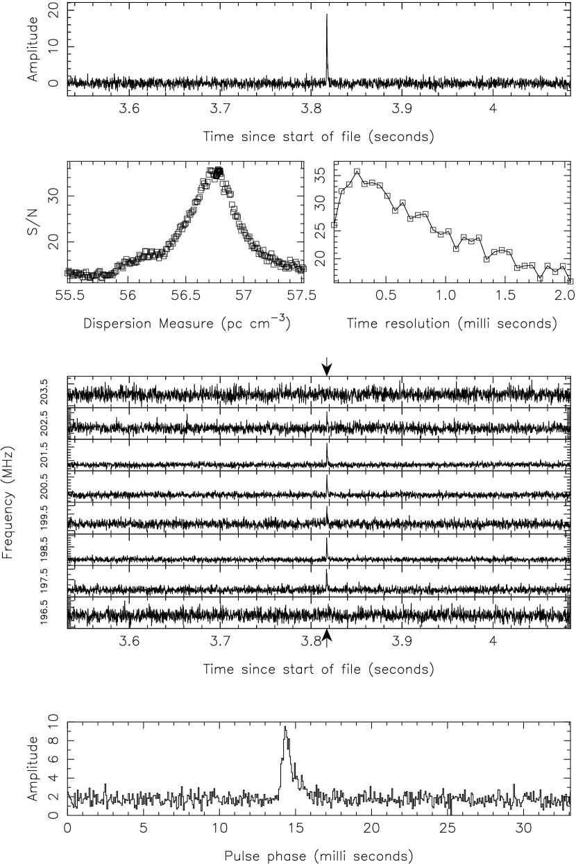
Figure 1: A bright giant pulse detected with the MWA-LFD early deployment system. Top: Dedispersed time series of a short data segment near the giant pulse. Middle panels: Diagnostic plots from the giant pulse search processing; plots of signal-to-noise ratio vs dispersion measure and time resolution, and dedispersed time series for 8 sub-bands, each 1 MHz wide, within the 8 MHz bandwidth. Bottom: The dedispersed pulse shown in high time resolution. The scattering tail is clearly visible.

2.3.2 Dedispersion and Giant Pulse Search

Our phased-array data streams were written out in the form of voltage samples (i.e., baseband data format), and hence allowed a coherent dedispersion to be performed on the signal. This procedure removes the dispersion entirely, and is especially important at low radio frequencies where the signal degradation due to dispersion can be rather severe. The dedispersed data are then subjected to the pulse detection algorithm to search for giant pulses. The procedures we have adopted are very similar to that described in Knight et al. (2006). The voltage samples are first Fourier transformed to the frequency domain and the spectra are divided into a series of sub-bands. Each sub-band is then multiplied by an inverse response filter (kernel) for the ISM (e.g. Hankins & Rickett, 1975), and then Fourier transformed back to the time domain to construct a time series with a time resolution coarser than the original data. By splitting the input signal into several sub-bands, the dispersive smearing is essentially reduced to that of an individual sub-band. This also means the procedure uses shorter transforms than single-channel coherent dedispersion and is consequently a more computationally efficient method.

This “coherent filterbank” stream of data are then square-law detected and combined after correcting for dispersive delays between the sub-bands, to construct a single coherently dedispersed time series for the entire band. The pulse detection procedure involved progressive smoothing (convolution) of time series with matched filters of widths ranging from 64 $\mu$s to 2048 $\mu$s in steps of a factor two, and identifying the intensity samples that exceed a set threshold (e.g. 8.5 $\sigma$). In addition to performing dedispersion at the Crab’s nominal DM of 56.791 ${\rm pc\ cm^{-3}}$ , we also perform this procedure over a large number of adjacent DM values (typically over a DM range $\approx$0.1${\rm DM_{crab}}$, in steps of 0.01 ${\rm pc\ cm^{-3}}$ ), in order to confirm the dispersion signature. For each DM and the matched filter width, we compute signal-to-noise ratio (S/N) of the pulse amplitude over a short stretch of time centered on the pulse. This process is computationally intensive and was carried out on Swinburne’s supercomputer. From this analysis, diagnostic plots are generated for each candidate giant pulse as shown in Fig. 1. We also check if the signal is broadband by displaying the dedispersed time series in 8 x 1 MHz sub-bands. These diagnostic plots were subjected to a careful human scrutiny to discriminate real giant pulses from spurious signals.

2.3.3 System Sensitivity and Flux Calibration

The Crab Nebula is a fairly bright and extended source in the radio sky, with a flux density of $\sim$955$~{}\nu^{-0.27}$ Jy (Bietenholz et al., 1997) and a characteristic diameter of $\sim$5^′.5. Thus, in general, for most conventional observations with large single-dish telescopes such as Arecibo and Parkes, the nebular emission dominates the system noise temperature (e.g. Cordes et al., 2004). However, in our case the combination of a low antenna gain, large sky background, high system temperature, large field of view, and significant side lobes of the antenna response function, leads to a very different scenario whereby the system temperature ${\rm T_{sys}}$ is heavily dominated by the sky background itself. This is further compounded by the fact that the tile response pattern becomes more complex at large zenith angles that are relevant for the Crab, and varies significantly over the duration of the observation depending on the zenith angle (ZA). Further technical aspects of the ED system are discussed by Bowman et al. (2006).

In order to account for these effects, and to obtain a realistic estimate of the sky background temperature, ${\rm T_{sky}}$ , we convolve the sky model, ${\rm T_{sky}}$ ($\theta$), with the antenna power response function, W($\theta$). The sky model ${\rm T_{sky}}$ ($\theta$) is obtained by extrapolation of the 408 MHz sky map of Haslam et al. (1982) assuming a spectral index $\alpha$ = $-2.6$. For our purpose, ${\rm W(\theta)}$ is the phased-array beam pattern when the tile beam is pointed toward the Crab. Performing the above calculation yields ${\rm T_{sky}}$ = 180 K when the Crab is at transit (ZA = 48^∘), but may increase as much as by 20% at larger zenith angles of the Crab (e.g. ZA = 60^∘). The net system temperature is given by ${\rm T_{sys}}$ = ${\rm T_{sky}}$ + ${\rm T_{recv}}$ , where ${\rm T_{recv}}$ is the receiver temperature. For the ED system, the receiver temperature is a strong function of frequency, and is $200\pm 20$ K near 200 MHz (Bowman et al., 2006). Thus ${\rm T_{sys}}$ = 380$\pm$30 K at 200 MHz, taking into account the nominal uncertainty in receiver temperature measurements and change in ${\rm T_{sky}}$ with the ZA.

In order to translate our system temperature estimates to their equivalent flux densities (i.e., the system equivalent flux density, ${\rm S_{sys}}$ ), we require an estimate for the array gain, G, expressed in conventional units of ${\rm K\,Jy^{-1}}$ . This gain parameter can be derived from the effective area of the tiles, ${\rm A_{eff}}$ , using the simple relation, ${\rm G=\mbox{${\rm A_{eff}}$\,}/2~{}\mbox{${\rm k_{B}}$\,}}$, where ${\rm k_{B}}$ is the Boltzmann constant. For the MWA-LFD antenna, the effective area is a strong function of frequency and is given by $\mbox{${\rm A_{eff}}$\,}=\lambda^{2}/x$, where $x$ is the frequency-dependent scaling parameter. Based on our design simulations $x=2.1$ at 200 MHz, i.e., $\mbox{${\rm A_{eff}}$\,}\approx 1~{}{\rm m^{2}}$ for a single dipole. Thus for the ED system which comprises 48 dipoles in total, the net effective area is $\approx$ 50 ${\rm m^{2}}$ at 200 MHz, i.e., an equivalent system gain of $\approx$0.02 ${\rm K\,Jy^{-1}}$ . However, as described in Bowman et al. (2006), the tile gain also has a strong functional dependence with the zenith angle. The measured dependence of ${\rm cos^{2.6}(ZA)}$ is quite steeper than a theoretically expected ${\rm cos^{2}(ZA)}$ form, and thus the nominal gain for the ED system is $\approx$0.008 ${\rm K\,Jy^{-1}}$ towards the Crab. Further, the zenith angle varies from $60^{\circ}$ (near rise or set) to $45^{\circ}$ (at transit) for the Crab, leading to a gain variation by a factor 2.5 over the observation. Thus, our ${\rm T_{sys}}$ estimate of 380 K corresponds to an equivalent system noise of ${\rm S_{sys}}$ = ${\rm T_{sys}}$ /G $\approx$ 47.5 kJy. For our recording bandwidth of 8 MHz and assuming a typical matched filter width of 250 $\mu$s, the effective ${\rm S_{sys}}$ is of the order of $\sim$1100 Jy, i.e., a minimum detectable pulse amplitude of $\sim$5.5 kJy for a 5-$\sigma$ detection threshold.

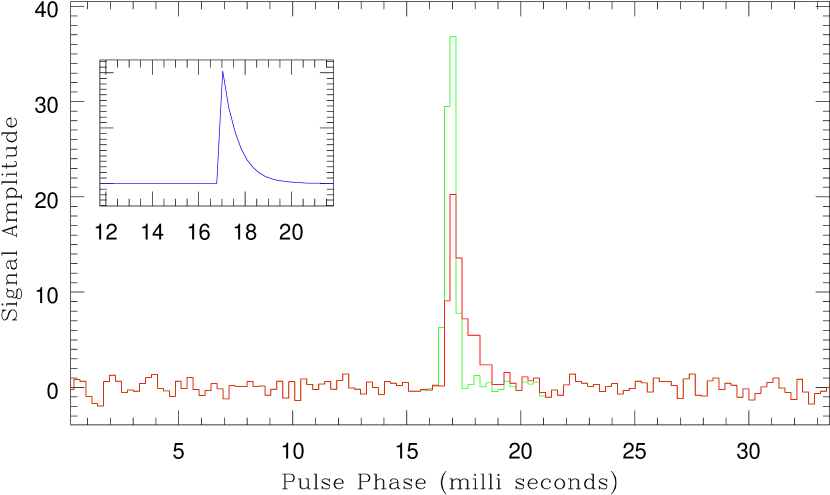
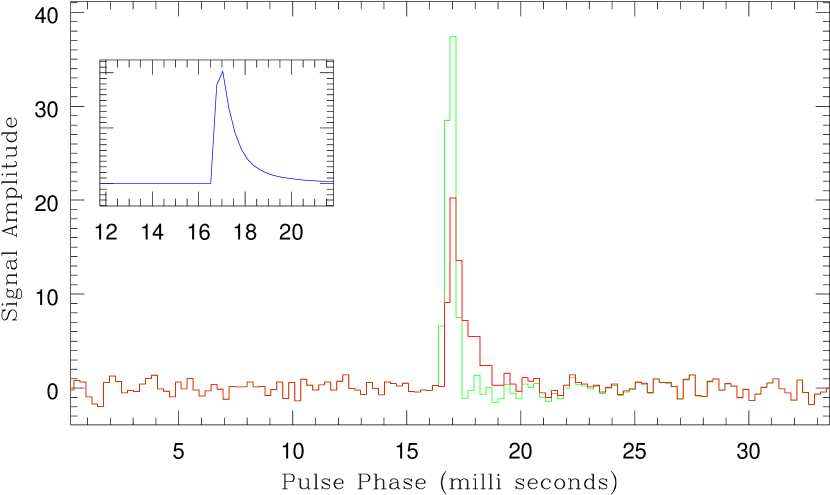
Figure 2: Measured and reconstructed pulse shapes of a bright giant pulse at 200 MHz. The best fit  scattering function (i.e., the pulse broadening function, PBF) is shown in the inset. The top and bottom panels correspond to different models of the PBF; an exponential PBF that corresponds to an infinite thin screen model of scattering medium (top), and a more rounded PBF that corresponds to a uniform distribution of scattering medium (bottom). The deconvolution results in a significant increase in  the peak signal strength and a pulse shape that is presumably closer to intrinsic.

2.3.4 Deconvolution of Pulse Broadening

Fig. 1 shows an example of giant pulse detection. As evident from this figure, the measured pulse shape is quite asymmetric and is marked by a clear lengthening at the trailing end, a characteristic of the pulse broadening phenomenon that results from multipath scattering in the intervening interstellar medium (ISM) (e.g. Williamson, 1972; Cordes & Lazio, 2001). This effect is more pronounced in observations of distant pulsars and at low frequencies (e.g. Bhat et al., 2004). The measured pulse shape, $y(t)$, can be modelled as effectively a convolution of the intrinsic pulse shape, $x(t)$, with the impulse response of the scattering medium, $g(t)$, often referred to as the pulse broadening function (PBF). More precisely,

$$y(t)=x(t)\otimes g(t)\otimes r(t)$$ (1)

where $r(t)$ is the net instrumental resolution function. The observed pulse broadening is usually quantified by a time scale, ${\rm\tau_{d}}$ , characteristic of a PBF fit to the measured pulse shape. The exact form of the PBF and its scaling with frequency depend on the nature of distribution of scattering material along the line-of-sight and on its wavenumber spectrum (e.g. Lambert & Rickett, 1999).

In order to estimate the pulse broadening, we adopt the CLEAN-based deconvolution approach developed by Bhat et al. (2003). Unlike the traditional frequency-extrapolation approach (e.g. Löhmer et al., 2001), this method makes no prior assumption of the intrinsic pulse shape, and thus offers a more robust means of determining the underlying PBF, and therefore can be applied to a wide variety of pulse shapes and degrees of scattering. The procedure involves deconvolving the pulse shape in a manner quite similar to the CLEAN algorithm used in synthesis imaging, while searching for the best-fit PBF and recovering the intrinsic pulse structure. It relies on a set of figures of merit that are defined in terms of positivity and symmetry of the resultant deconvolved pulse and some parameters characterizing the noise statistics in order to determine the best-fit PBF. Such an approach is especially justified for the Crab giant pulses, as they are known to show structures at timescales down to microseconds or even nanoseconds, and show complex and quite unusual evolution in pulse morphology with frequency.

The deconvolution procedure employed here is similar to that described in Bhat et al. (2003), except that the restoring function used in our case is a much simpler one. This is because the pulse smearing due to residual dispersion and instrumental effects is negligible. The major contributing factor to our restoring function is that due to time binning of the pulse profile. We used two different trial PBFs; the first, ${\rm g_{1}}$ , is appropriate for a thin slab scattering screen of infinite transverse extent (${\rm PBF_{1}}$ ), and the second, ${\rm g_{2}}$ , corresponds to a uniformly distributed scattering medium (${\rm PBF_{2}}$ ). Their functional forms are given by (e.g. Williamson, 1972),

$$g_{1}(t)=\tau_{d}^{-1}\exp(-t/\mbox{${\rm\tau_{d}}$\,})\,u(t),\qquad\qquad\qquad$$ (2)

$$g_{2}(t)=(\pi^{5}\tau_{d}^{3}/4t^{5})^{1/2}\exp(-\pi^{2}\mbox{${\rm\tau_{d}}$\,}/4t)\,u(t).$$ (3)

where $u(t)$ is the unit step function, $u(<0)=0,u(\geq 0)=1$. While ${\rm PBF_{1}}$ , which has a one-sided exponential form, has been commonly used by several authors in the past, the latter PBF is a generic proxy for more realistic distributions of scattering material. The best-fit PBFs obtained in this manner along with the respective intrinsic pulse shapes are shown in Fig. 2. As evident from this figure, the deconvolution process naturally leads to a significant increase (nearly by a factor two) in the effective signal-to-noise ratio of the pulse.

3 Results and Discussion

3.1 Giant Pulse Amplitudes and Brightness Temperatures

The measured amplitudes of giant pulses at low radio frequencies are determined by a number of factors such as the nature of the emission spectrum, the degree of scattering and the time resolution of the data. At frequencies $\scriptscriptstyle\stackrel{{\scriptstyle>}}{{\sim}}$  300 MHz, the pulse energies are known to follow a $\nu^{-4.5}$ form, i.e., a spectral form that is much steeper than typical pulsar spectrum. The behaviour of the spectrum at low frequencies is not well understood, although some of the early work suggests a turnover of the spectrum near our observing frequency of 200 MHz (e.g. Manchester & Taylor, 1977). Further, although the Crab pulsar is known to show quite a peculiar evolution in frequency in terms of pulse morphology and structure of both the average and giant pulse emission, at frequencies $\scriptscriptstyle\stackrel{{\scriptstyle<}}{{\sim}}$  300 MHz, scattering is likely to dictate the measured pulse shape as the pulse smearing becomes severe. Thus, even though the giant pulse emission inherently possesses structures down to microsecond or even nanosecond levels, finer structural details of individual giant pulses are simply not discernable due to severe broadening of the intrinsic pulse expected at these frequencies. Although in principle our deconvolution approach is useful for potentially extracting the information in such situations, unfortunately the signal-to-noise of our data does not seem large enough to attempt such an analysis. The effective time resolution of the data is also an important factor, as any level of smoothing (convolution) in time performed to aid either a detection of pulse, or an enhancement in the signal strength, would mean an inevitable reduction in the peak pulse amplitudes. Thus, in short, measurements of giant pulse amplitudes and fluxes at low frequencies should be treated with some caution, especially when compared with similar measurements made at higher frequencies.

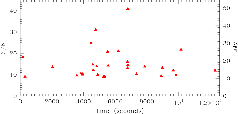
Figure 3: Summary plot of giant pulse detections at 200 MHz. The peak flux densities range from 10 to 50 kJy. Despite small-number statistics, these detections seem to follow a roughly power-law distribution in pulse amplitude and energy. In total, 31 pulses were detected in 3.5 hours of observations. The S/Ns shown are for the east-west polarisation; the signal is detected in north-south polarisation in most cases, albeit with a poorer S/N.

Results from our giant pulse search are summarised in Fig. 3 where the measured pulse amplitudes are plotted against their times of occurrence. The estimates of S/N are converted to units of Jy using the flux calibration procedures detailed in § 2.3.3. Note that these are the measured peak pulse amplitudes, i.e., no correction is applied for the enhancement in signal strength achievable by the deconvolution of scattering. Despite the small-number statistics, the pulse energies seem to follow a roughly power-law type distribution (index = $-1.7\pm 0.1$). For the nominal system temperature and gain estimates as described in § 2.3.3 (380 K and 0.01 ${\rm K\,Jy^{-1}}$ respectively), and given our typical processing parameters (a net bandwidth of 6 MHz and a nominal pulse width of 300 $\mu$s), the effective system noise turns out to be of the order $\sim$1100 Jy. This means our system is sensitive to pulses brighter than $\sim$9 kJy, assuming a 8.5-$\sigma$ detection threshold. Our search analysis has yielded a total of 31 giant pulses above this threshold. The brightest giant pulse detected in our data has a peak flux density of 50 kJy and and a width $\approx$300 $\mu$s. The measured amplitudes can be translated to implied brightness temperatures (${\rm T_{b}}$ ) using a simple relation (based on the light-travel size and ignoring relativistic dilation),

$$\mbox{${\rm T_{b}}$\,}=\left({\mbox{${\rm S_{\nu}}$\,}\over 2\,\mbox{${\rm k_{B}}$\,}}\right)\left({{\rm D}\over\nu\mbox{${\Delta t}$\,}}\right)^{2},$$ (4)

where ${\rm S_{\nu}}$ is the peak flux density and ${\Delta t}$ is the pulse width; ${\rm k_{B}}$ is the Boltzmann constant and D corresponds to the Earth-pulsar distance. Assuming a peak pulse amplitude of 100 kJy (i.e., the amplitude of the reconstructed pulse in Fig. 2) and a nominal distance of 2 kpc to the Crab Nebula (e.g. Cordes & Lazio, 2002), we estimate a brightness temperature of $10^{31.6}$ K for our brightest giant pulse. However this is likely to be an underestimate of the true brightness temperature given the degradation of the signal strength expected due to pulse broadening. Interestingly, this estimate is comparable to that derived from the brightest giant pulse  detected at 430 MHz using Arecibo (Cordes et al., 2004) where the scattering is at least an order of magnitude smaller. Indeed much higher brightness temperatures ($10^{37}$ K) have been reported from observations at 5.5 GHz (where the scattering is negligibly small) made at nanosecond time resolutions (Hankins et al., 2003). Despite the various factors that degrade the signal strength at low frequencies, our observations confirm fairly high brightness temperatures for the giant pulses at 200 MHz.

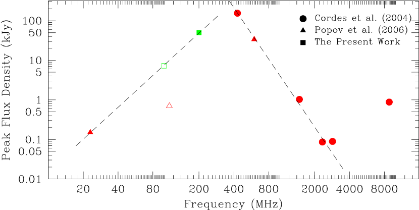
Figure 4: Peak flux densities of the brightest giant pulses (in 1 hr) over a wide range of frequencies from 23 MHz to 8.8 GHz (solid symbols). The symbols indicate data from different sources – circles denote Arecibo observations of Cordes et al. (2004), triangles are recent low frequency observations of Popov et al. (2006), and squares denote the present work. The unfilled symbols near 100 MHz indicate limits derived from a non-detection with MWA-LFD (square) and the brightest giant pulse in 15 minutes of observation (triangle).

The amplitude of the brightest giant pulse detected in our data is compared with similar estimates from recent observations in Fig. 4. The plot spans a wide range of frequencies from $\sim$20 MHz to $\sim$9 GHz, i.e., nearly 3 orders in magnitude. Observations at most of the higher frequencies are from an intensive multifrequency campaign with Arecibo (Cordes et al., 2004), while those at 23, 111 and 600 MHz are from the recent work of Popov et al. (2006). From our non-detection at 100 MHz, we derive an upper limit of $\sim$5 kJy for the bright giant pulses detectable at this frequency, by assuming a simple $\nu^{-2.6}$ scaling of our measured ${\rm T_{sky}}$ and nominal values for the anticipated system sensitivity. This is much larger than the 0.7 kJy value for the brightest observed pulse reported by Popov et al. (2006). However, this discrepancy can be attributed to the fact that it is based on a much shorter observing duration (15 min) and hence may not have been quite sensitive to the tail end of the giant pulse power-law distribution. It is still interesting that the measured peak amplitudes of the brightest giant pulses in one hour follow roughly power-law trends with frequency, with an empirical relation of the form $\nu^{-4.3\pm 0.2}$ at frequencies $\scriptscriptstyle\stackrel{{\scriptstyle>}}{{\sim}}$  300 MHz (i.e., comparable to the nominal spectral slope of giant pulse energies), and $\nu^{+2.7\pm 0.1}$ at lower frequencies (if we exclude the 111 MHz value). While it is harder to extract any meaningful information about the nature of the spectrum from these measurements alone, this plot may still serve as a useful guide to assess the detection prospects of bright giant pulses. Characterization of the spectrum requires reliable measurements of average giant pulse fluxes or energies, which are not easily obtainable for all these frequencies. Clearly, scattering will strongly influence the giant pulse detection prospects within the MWA-LFD’s frequency range. We discuss the detection prospects for the full system in § 4.

3.2 Implications of Measured Pulse Broadening

Our pulse deconvolution yields a ${\rm\tau_{d}}$ of $670\pm 100$ $\mu$s for the PBF ${\rm g_{1}}$ , and $395\pm 50$ $\mu$s for the PBF ${\rm g_{2}}$ . As described in Bhat et al. (2004), in principle, the figures of merit of the CLEAN deconvolution technique can be used to assess which PBF better fits the data. Specifically, their parameter, $f_{r}$, which is a measure of positivity, can be treated as a useful indicator of “goodness” of the CLEAN subtraction. We expect $f_{r}~{}\mbox{\raisebox{-0.43057pt}{$\scriptscriptstyle\stackrel{{\scriptstyle<}}{{\sim}}$\,}}~{}1$ for successfully deconvolved pulses, while larger values imply slightly overCLEANed pulses. For the results in Fig. 2, we obtain values of 1.3 and 0.85 respectively for deconvolution with ${\rm PBF_{1}}$ and ${\rm PBF_{2}}$ , which would mean ${\rm PBF_{2}}$ is probably a better fit to the data. As ${\rm PBF_{2}}$ represents a scattering geometry with distributed material, this suggests that much of the observed scattering is possibly due to the intervening ionized gas along the Earth-pulsar line-of-sight.

Our ${\rm\tau_{d}}$ estimates for the two PBFs differ roughly by a factor two, and this  is because ${\rm\tau_{d}}$ has different meanings for the two scenarios. For ${\rm PBF_{1}}$ , ${\rm\tau_{d}}$ is both $e^{-1}$ point of the distribution and the expectation value of $t$, whereas for ${\rm PBF_{2}}$ , ${\rm\tau_{d}}$ is close to the maximum of the distribution, which is at $(\pi^{2}/10)\mbox{${\rm\tau_{d}}$\,}=0.99~{}\mbox{${\rm\tau_{d}}$\,}$, while the expectation value of $t$ is $(\pi^{2}/2)\mbox{${\rm\tau_{d}}$\,}=4.93~{}\mbox{${\rm\tau_{d}}$\,}$ (see eqn. 3).

The measured pulse broadening can be used to infer the scattering measure (SM), defined as ${\rm SM}\equiv\int_{0}^{D}ds\,\mbox{${C_{n}^{2}}$\,}(s)$, where ${C_{n}^{2}}$  is the spectral coefficient of the wavenumber spectrum of electron density irregularities in the ISM and D is the Earth-pulsar distance. It signifies the total amount of scattering along the line-of-sight and depends critically on the nature of distribution of the scattering material. It can be related to pulse broadening via the relation $\mbox{${\rm\tau_{d}}$\,}\approx 1.1\,\mbox{$W_{\tau}$}~{}{\rm SM}^{6/5}\nu^{-4.4}D$, where $\nu$ is in GHz, D is in kpc, and $W_{\tau}$ is a geometric factor that depends on the line-of-sight distribution of scattering material (Cordes & Rickett, 1998). Using this relation, and assuming $W_{\tau}$ = 1 , we estimate the effective SM for a uniform medium as $(1\pm 0.3)\times 10^{-3}$ ${\rm kpc\ m^{-20/3}}$ . This can be compared to a value $1.7\times 10^{-3}$ ${\rm kpc\ m^{-20/3}}$ as predicted by the NE2001 model (Cordes & Lazio, 2002).

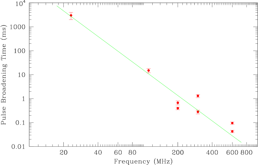
Figure 5: Low frequency measurements of pulse broadening time from recent observations of the Crab pulsar. Observations at 23, 111 and 600 MHz are from Popov et al. (2006), while those at 300 MHz and the higher value at 600 MHz are from Sallmen et al. (1999). The solid line shows our best-fit scaling ($\mbox{${\rm\tau_{d}}$\,}\propto\nu^{-3.5\pm 0.2}$) to the data (excluding higher values at 300 and 600 MHz), which is significantly shallower than the $\nu^{-4.4}$ scaling expected from a Kolmogorov model. Our measurements (at 200 MHz) are $\sim$3–5 times smaller than that predicted based on the published measurements and frequency scaling.

While the estimates of pulse broadening time are, in general, reliable measures of the integrated scattering due to the ISM, some caution is needed while interpreting the measurements for the Crab pulsar. This is because the material within or around the nebula can potentially influence, or may even dominate, the observed scattering on some (or most) occasions. In fact, observations have shown that the dispersion and scattering measurements of the Crab vary significantly with time (Rankin & Counselman, 1973; Lyne & Thorne, 1975; Isaacman & Rankin, 1977; Backer, 2000; Lyne et al., 2001). The extreme cases are the so-called “scattering events” where the pulse-broadening time increased dramatically (by two orders of magnitude) and subsequently decreased to normal over a period of several months (Lyne & Thorne, 1975). Such anomalies were interpreted in terms of an increase in turbulence or density within the nebular region. Barring such exceptional cases, the measurements of pulse-broadening time at any given frequency still show large variations from one epoch to the other. For example, Sallmen et al. (1999) reported the broadening time changing from 0.28 to 1.3 ms from their Green Bank observations at 300 MHz. More recently, Popov et al. (2006) measured a value of $43\pm 5$ $\mu$s at 600 MHz, which is a factor two smaller than that reported by Sallmen et al. (1999) at this frequency. Fig. 5 shows a summary of these measurements along with those from our observations. Incidentally, our measurements are $\sim$3–5 times smaller than that predicted based on the published measurements and frequency scaling. This may suggest that the nebular contribution to the total scattering is now smaller compared to those in earlier observations. In other words, the bulk of our observed scattering is likely resulting from the distributed ISM along the line-of-sight. The best-fit frequency scaling of $\mbox{${\rm\tau_{d}}$\,}\propto\nu^{-3.5\pm 0.2}$ derived by us (Fig. 5) is in agreement with that of Popov et al. (2006) but is a significant departure from a Kolmogorov scaling ($\nu^{-4.4}$) favored by some of the earlier observations (Isaacman & Rankin, 1977; Sallmen et al., 1999), when the bulk of the observed scattering was attributed to material either inside or around the synchrotron nebula.

In summary, our measurement of a low scattering and an SM estimate that is somewhat lower than that predicted by the NE2001 electron density model (which largely accounts for the scattering due to the distributed ISM), suggest that the contribution from the nebula itself is probably at its lowest. This is further supported by a reasonably good fit obtained with ${\rm PBF_{2}}$ which corresponds to a distributed scattering geometry. If the scattering due to the nebula was dominant, one would have expected the measured pulse, and the implied PBF, to have quite different shape given the filamentary structures of the nebular material. Such filaments would mean scattering structures with  large axial ratios, which may produce PBFs that are of the form ${\rm\propto t^{-1/2}exp(-t)}$ and possibly truncated beyond certain times (e.g. Cordes & Lazio, 2001). Interestingly, this measurement of low scattering is also consistent with our recent observations at a frequency of 1400 MHz made with the ATCA, where we estimate the pulse broadening to be $\scriptscriptstyle\stackrel{{\scriptstyle<}}{{\sim}}$  1 $\mu$s (Bhat et al., 2007). Finally, we believe such a low scattering is what enabled a successful detection of the giant pulses with our ED system. For instance, if the scattering was to be dominated by the nebula, increasing the net pulse broadening by a factor 5 to 10, then the peak amplitude of the pulse will be reduced by a similar factor, rendering a positive detection rather difficult with our simple equipment. All in all, the measurement of a low scattering and our detection prospects are coupled, and perhaps it is a coincidence that our observations were made at an epoch when the scattering happened to be unusually low.

4 Giant Pulse Detection Prospects with the Full MWA-LFD System

Our successful detection of the Crab giant pulses with the ED system opens up some exciting prospects for the studies of giant pulses and other fast radio transients with the full MWA-LFD system when it becomes operational. The full system will have a sensitivity that is over two orders of magnitude larger than the ED system, and in combination with a much larger bandwidth feasible for data recording and the instrument’s unique capability to observe at more than one frequency simultaneously, the MWA-LFD will offer some brand new avenues of investigation in this arena.

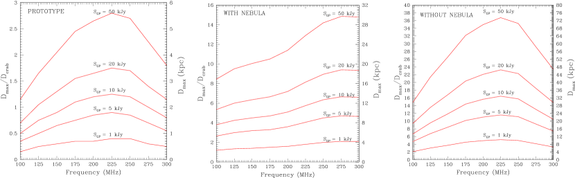
Figure 6: Giant pulse detection sensitivity of the MWA-LFD system. The sensitivity is expressed as maximum distance Dmax to which a giant pulse is potentially detectable. For the prototype system (left panel), the achievable sensitivity is dominated by the system noise itself, and an optimal performance is expected near 200 MHz. The middle and right panels show projected sensitivities for the full system. The nebular emission is important for “Crab-like” pulsars that reside in “Crab-nebula-like” environment (middle panel). The nebular contribution to the system noise decreases significantly above 190 MHz as the nebula is resolved by the array beam (assuming an array diameter  of $\approx$1 km), thus significantly increasing the system sensitivity at these frequencies. For field pulsars however (right panel), Dmax is largely determined by the sensitivity of the array itself, with the best performance expected near 200 MHz.

Fig. 6 shows giant pulse detection prospects of the MWA-LFD system, where the sensitivity curves for the full system are shown (middle and right panels) along with those for the prototype ED system (left panel). The sensitivity curves are dramatically different for the two cases, which is due to an interplay of different factors involved in the calculations. For the ED system, the system noise dominates over all other contributions and a maximum in sensitivity is expected near 200 MHz. For “Crab-like” pulsars that reside in “Crab-nebula-like” environment, the sensitivity calculations take into consideration factors such as, contribution from the nebular emission to the system noise, as well as frequency dependencies of the basic system performance parameters (i.e., ${\rm T_{sys}}$ and G) and the sky background (${\rm T_{sky}}$ ). The combination of a decreasing  ${\rm T_{sky}}$ and a reduced nebular contribution as the nebula becomes resolved at higher frequencies make up for the decrease in tile gain and a larger ${\rm T_{sys}}$ expected at higher frequencies. This effectively yields higher sensitivity at frequencies $\scriptscriptstyle\stackrel{{\scriptstyle>}}{{\sim}}$ 200 MHz. Naturally, much higher sensitivities can be achieved for field pulsars with no nebular background, where ${\rm D_{max}}$ is largely determined by the system performance parameters such the array gain and noise temperature.

To elaborate further on our sensitivity calculations, the radiometer equation can be re-written for the case of giant pulse detection as (see e.g. McLaughlin & Cordes (2003); Cordes et al. (2004)),

$${\rm\left({S\over N}\right)_{det}}=~{}{\rm D}^{-2}\left({\mbox{${\rm S_{GP}}$\,}\over\mbox{${\rm S_{sys}}$\,}}\right)\left(\mbox{${\rm N_{pol}}$\,}\mbox{${\Delta\nu}$\,}\mbox{${\rm W_{p}}$\,}\right)^{{1\over 2}}$$ (5)

where ${\rm(S/N)_{det}}$ is the signal-to-noise achievable for a giant pulse of peak amplitude ${\rm S_{GP}}$ using a system of sensitivity ${\rm S_{sys}}$ , with ${\Delta\nu}$ being the bandwidth over which the data are recorded and ${\rm W_{p}}$ is the effective pulse width, and ${\rm N_{pol}}$ is the number of polarizations that are summed. Conversely, for a given system with sensitivity ${\rm S_{sys}}$ , the maximum distance to which a giant pulse of amplitude ${\rm S_{GP}}$ is potentially detectable is given by

$$\mbox{${\rm D_{max}}$\,}=\left({\rm{S\over N}}\right)^{-{1\over 2}}\left({\mbox{${\rm S_{GP}}$\,}\over\mbox{${\rm S_{sys}}$\,}}\right)^{{1\over 2}}\left(\mbox{${\rm N_{pol}}$\,}\mbox{${\Delta\nu}$\,}\mbox{${\rm W_{p}}$\,}\right)^{{1\over 4}}$$ (6)

For the MWA-LFD system, ${\rm S_{sys}}$ is a strong function of the observing frequency, as both the system temperature and gain vary significantly with frequency (Bowman et al., 2006). Further, the full array will comprise 512 tiles spread over a region of $\sim$1 km. Thus, both the effective gain and resolution of the array (i.e., half-power width of the phased array beam pattern) are such that ${\rm S_{sys}}$ is strongly influenced by the nebula. For an array layout extending out to 1 km, the nebula remains unresolved at the lower half of the MWA-LFD’s operating frequency range, but becomes resolved near 200 MHz, where the effective resolution (beam width) becomes comparable to the Crab’s characteristic diameter ($5.^{\prime}$5). The net system sensitivity (in units of Jy) is thus given by $\mbox{${\rm S_{sys}}$\,}(\nu)=\mbox{${\rm S_{sys0}}$\,}(\nu)+\mbox{${\rm f_{\nu}}$\,}\mbox{${\rm S_{CN}}$\,}(\nu)$, where ${\rm S_{sys0}}$  is the system sensitivity without the nebular contribution to the system noise and ${\rm f_{\nu}}$ is the beam dilution factor, given by $\mbox{${\rm f_{\nu}}$\,}=\Omega_{A}(\nu)/\Omega_{CN}$ where ${\rm\Omega_{A}}$ and ${\rm\Omega_{CN}}$ are the solid angle areas of the phased array beam and the nebula, respectively. The system sensitivity when pointed away from the nebula is ${\rm\mbox{${\rm S_{sys0}}$\,}(\nu)=\mbox{${\rm T_{sys0}}$\,}(\nu)/G(\nu)}$, where $\mbox{${\rm T_{sys}}$\,}(\nu)=\mbox{${\rm T_{sky}}$\,}(\nu)+\mbox{${\rm T_{recv}}$\,}(\nu)$ is the net system temperature. Furthermore, the nebular emission is also frequency dependent (see § 2.3.3), and the integrated flux density is expected to change as much as by 30% over the MWA-LFD’s frequency range.

Thus, in the lower half of the MWA-LFD frequency range (100–200 MHz), sensitivity is largely determined by the combination of a decrease in ${\rm T_{sky}}$ and an increase in the tile gain, and then sharply increases near mid-way as the nebula becomes resolved (Fig. 6). A giant pulse as bright as the brightest one in our data is thus potentially detectable with the full system out to a distance of $\sim$17 kpc at 100 MHz and out to $\sim$30 kpc at 300 MHz. Indeed these limits will be even larger in the case of giant-pulse emitters that do not reside in a nebula. In short, bright giant pulses are potentially detectable over a wide range of Galactic distances within the full range of MWA-LFD frequencies.

The brightest giant pulse detected in our data (${\rm S_{GP}}$ = 50 kJy) has an energy content of $\sim 1.85\times 10^{5}$ kJy $\mu$s. Although our ED system is not capable of detecting the integrated emission from the pulsar, assuming a pulsar flux density of $\sim 650$ mJy at 400 MHz and a spectral index of $-$3.1 (e.g. Manchester et al., 2005), it turns out such a giant pulse will be at least $\sim 100$ times more energetic than the average emission (if we assume the spectrum does not turn over until $\sim$200 MHz). Given this, and an expected two orders of magnitude improvement in sensitivity for the full array, it is quite likely that almost all pulses emitted through the giant-pulse emission mechanism (say, energy $\mbox{\raisebox{-0.43057pt}{$\scriptscriptstyle\stackrel{{\scriptstyle>}}{{\sim}}$\,}}10\times$ the average emission) will be potentially detectable with the full system at 200 MHz. This will enable a detailed characterisation of the giant pulses and their energy distributions at low frequencies, a poorly studied aspect of the Crab giant pulses.

It is worthwhile to examine the detection prospects for other known giant-pulse–emitters such as PSRs B0540–69 and B1937+21. PSR B0540–69 is a young, Crab-like pulsar located inside the Large Magellanic Cloud (D $\sim$ 50 kpc), for which the giant-pulse energy distribution is known to follow the form $P(E>E_{o})=KE_{o}^{-\alpha}$; where P is the probability of emitting a giant pulse with energy greater than $E_{o}$ (in units of the average pulse energy), and $K$=0.26 and $\alpha\sim 1.8$ from Johnston et al. (2004). The pulsar period is 50.35 ms and thus the strongest pulse emitted in 1 hr will have an energy $E_{o}\sim 235\langle E\rangle$ where $\langle E\rangle$ is the average emission. Assuming giant pulses dominate the pulsar emission and a spectral index of $-$3.6 (and no spectral turnover down to $\sim$200 MHz), we estimate the pulsar flux to be 27 mJy at 200 MHz, thus a giant pulse with energy 235$\langle E\rangle$ would imply $3.3\times 10^{2}$ kJy $\mu$s. This is 56 times weaker than our brightest giant pulse, or 20 times below the detection threshold of the ED system. However, with the full array ($\sim$170 times improvement in sensitivity), such a giant pulse should be detectable with S/N $\sim$ 85. And given the $KE_{o}^{-\alpha}$ form for the energy distribution, we estimate $\sim 50$ pulses to be potentially detectable in 1 hr of observation.

For the millisecond pulsar B1937+21, the giant-pulse energies follow a similar power-law form with K=0.032 and $\alpha\sim 1.8$ at 430 MHz (Cognard et al., 1996). Following similar arguments as above, we estimate the brightest giant pulse from this pulsar in 1 hr will be $\sim 500$ times as energetic as its average emission. While this is 8 times below the detection threshold of our ED system, it will be easily detectable (S/N $\sim$ 212) with the full array and assuming a power-law index of 1.8, we estimate there to be as many as $\sim$ 250 giant pulses with S/N $>10$ in 1 hr duration. While these are only some rough estimates, and do not take into consideration the impact of increased scattering at low frequencies, it is evident that the full system offers exciting prospects for giant pulse studies in general.

While the above calculations are specifically performed for giant pulses, the same treatment also applies to fast radio transients of similar characteristics (i.e., time scales of the order of 100 $\mu$s or longer). The superb RFI-quiet environment of the proposed MWA-LFD site can be exploited to take the best advantage of this potential. Moreover, the instrument’s capabilities such as multibeaming will serve as powerful discriminators of real versus spurious signals. Thus the full system is indeed a promising instrument for science related to giant pulses and similar fast radio transients at low frequencies.

5 Conclusions and Future Work

Using a simple equipment operating in the Western Australian outback, we have successfully detected giant pulses from the Crab Nebula pulsar at a frequency of 200 MHz. Despite a large sky background severely limiting the sensitivity achievable at such low frequencies, our system, comprising just three tiles, each consisting of a 4 x 4 array of dipoles, detected a total of 31 giant pulses over a duration of 3.5 hours. The measured pulse shape is significantly broadened by multipath scattering due to the ISM, and results in a degradation of the intrinsic pulse amplitude by nearly a factor of two. The deconvolution of the measured pulse using a CLEAN-based procedure yields a pulse-broadening time of 670$\pm$100 $\mu$s for the case of a thin slab scattering model, and 400$\pm$50 $\mu$s for a model where the scattering material is uniformly distributed along the line of sight. The implied degree of scattering is the lowest that has been reported towards the Crab pulsar from observations made so far. In fact, our detection of giant pulses in such large numbers would not have been possible but for such low level of scattering. Together with recent observations at low frequencies, our measurements of the pulse-broadening time support a shallow scaling in frequency ($\mbox{${\rm\tau_{d}}$\,}\propto\nu^{-3.5\pm 0.2}$). With the sensitivity of our equipment (a gain of $\sim$0.01 ${\rm K\,Jy^{-1}}$ and a system temperature of $\sim$400 K towards the Crab), pulses that are brighter than $\sim$9 kJy in amplitude are easily detected. The brightest giant pulse detected in our data has a peak amplitude of $\sim$50 kJy and a width of $\approx$300 $\mu$s, and the equivalent brightness temperature is $10^{31.6}$ K, assuming a pulsar distance of 2 kpc.

The success of our exploratory observations underscores the tremendous potential the full MWA-LFD system will offer for studies of pulsar science in general, and for giant pulses and fast transients in particular, at low radio frequencies. With a sensitivity that is over two orders of magnitude larger than that of the prototype equipment, the full system will have the capability to detect giant pulses over a wide range of Galactic distances. For instance, giant pulses as bright as $\sim$50 kJy will be potentially detectable out to a distance of  $\sim$30 kpc in the case of Crab-like pulsars, and even further in the case of objects that do not reside in a nebula. In addition to enabling an in-depth study of Crab giant pulses at frequencies $\scriptscriptstyle\stackrel{{\scriptstyle<}}{{\sim}}$ 300 MHz, the MWA-LFD will be a promising instrument for a wide variety of pulsar and transient science at low frequencies.

Acknowledgements: Data processing for the work presented here was carried out at the Swinburne supercomputing facility, and data storage resources were provided by the GrangeNet facility, Canberra, ACT. We thank S. Tingay and Y. Gupta for valuable discussions pertaining to the phased-array realisation of the ED array, and C. West and P. Fuggle for assistance with the GrangeNet access by the Swinburne supercomputer. The prototype field deployment effort for the MWA-LFD project was supported by the MIT School of Science, the MIT Haystack Observatory, University of Melbourne, Australian National University, Curtin University, Australian National Telescope Facility, University of Western Australia, Harvard-Smithsonian Center for Astrophysics, Mileura Cattle Company, the government of Western Australia, the Australian Research Council and the U.S. National Science Foundation.

References

- Argyle & Gower (1972) Argyle, E., & Gower, J. F. R. 1972, ApJ, 175, L89
- Backer (2000) Backer, D. C. 2000, ASP Conf. Ser. 202: IAU Colloq. 177: Pulsar Astronomy - 2000 and Beyond, 202, t493
- Bhat et al. (2003) Bhat, N. D. R., Cordes, J. M. & Chatterjee, S. 2003, ApJ, 584, 782
- Bhat et al. (2004) Bhat, N. D. R., Cordes, J. M., Camilo, F., Nice, D. J., & Lorimer, D. R. 2004, ApJ, 605, 759
- Bhat et al. (2007) Bhat, N. D. R., et al. 2007, In preparation
- Bietenholz et al. (1997) Bietenholz, M. F., Kassim, N., Frail, D. A., Perley, R. A., Erickson, W. C., & Hajian, A. R. 1997, ApJ, 490, 2991
- Briggs et al. (2007) Briggs, F. H., et al. 2007, In preparation
- Bowman et al. (2006) Bowman, J. D., et al. 2006, AJ, Accepted
- Cognard et al. (1996) Cognard, I., Shrauner, J. A., Taylor, J. H., & Thorsett, S. E. 1996, ApJ, 457, L81
- Cordes et al. (2004) Cordes, J. M., Bhat, N. D. R., Hankins, T. H., McLaughlin, M. A., & Kern, J. 2004, ApJ, 612, 375
- Cordes & Lazio (2001) Cordes, J. M., & Lazio, T. J. W. 2001, ApJ, 549, 997
- Cordes & Lazio (2002) Cordes, J. M. & Lazio, T. J. W. 2002, astro-ph/0207156
- Cordes & Rickett (1998) Cordes, J. M., & Rickett, B. J. 1998, ApJ, 507, 846
- Hankins et al. (2003) Hankins, T. H., Kern, J. S., Weatherall, J. C., & Eilek, J. A. 2003, Nature, 422, 141
- Hankins & Rickett (1975) Hankins, T. H., & Rickett, B. J. 1975, Methods in Computational Physics. Volume 14 - Radio astronomy, 14, 55
- Haslam et al. (1982) Haslam, C. G. T., Salter, C. J., Stoffel, H., & Wilson, W. E. 1982, A&AS, 47, 1
- Isaacman & Rankin (1977) Isaacman, R., & Rankin, J. M. 1977, ApJ, 214, 214
- Johnston et al. (2004) Johnston, S., Romani, R. W., Marshall, F. E., & Zhang, W. 2004, MNRAS, 355, 31
- Knight et al. (2006) Knight, H. S., Bailes, M., Manchester, R. N., Ord, S. M., & Jacoby, B. A. 2006, ApJ, 640, 941
- Lambert & Rickett (1999) Lambert, H. C., & Rickett, B. J. 1999, ApJ, 517, 299
- Löhmer et al. (2001) Löhmer, O., Kramer, M., Mitra, D., Lorimer, D. R., & Lyne, A. G. 2001, ApJ, 562, L157
- Lundgren et al. (1995) Lundgren, S. C., Cordes, J. M., Ulmer, M., Matz, S. M., Lomatch, S., Foster, R. S., & Hankins, T. 1995, ApJ, 453, 433
- Lyne et al. (2001) Lyne, A. G., Pritchard, R. S., & Graham-Smith, F. 2001, MNRAS, 321, 67
- Lyne & Thorne (1975) Lyne, A. G., & Thorne, D. J. 1975, MNRAS, 172, 97
- Manchester et al. (2005) Manchester, R. N., Hobbs, G. B., Teoh, A., & Hobbs, M. 2005, AJ, 129, 1993
- Manchester & Taylor (1977) Manchester, R. N., & Taylor, J. H. 1977, Pulsars (W. H. Freeman, San Francisco, CA, U.S.A.)
- McLaughlin & Cordes (2003) McLaughlin, M. A., & Cordes, J. M. 2003, ApJ, 596, 982
- Moffett & Hankins (1996) Moffett, D. A., & Hankins, T. H. 1996, ApJ, 468, 779
- Popov et al. (2006) Popov, M. V., et al. 2006, Astronomy Reports, 50, 562
- Rankin et al. (1970) Rankin, J. M., Comella, J. M., Craft, H. D., Jr., Richards, D. W., Campbell, D. B., & Counselman, C. C., III 1970, ApJ, 162, 707
- Rankin & Counselman (1973) Rankin, J. M., & Counselman, C. C., III 1973, ApJ, 181, 875
- Sallmen et al. (1999) Sallmen, S., Backer, D. C., Hankins, T. H., Moffett, D., & Lundgren, S. 1999, ApJ, 517, 460
- Staelin & Reifenstein (1968) Staelin, D. H., & Reifenstein, E. C. 1968, Science, 162, 1481
- Williamson (1972) Williamson, I. P. 1972, MNRAS, 157, 55