Observational bounds on the cosmic radiation density

Abstract

We consider the inference of the cosmic radiation density, traditionally parameterised as the effective number of neutrino species $N_{\rm eff}$, from precision cosmological data. Paying particular attention to systematic effects, notably scale-dependent biasing in the galaxy power spectrum, we find no evidence for a significant deviation of $N_{\rm eff}$ from the standard value of $N_{\rm eff}^{0}=3.046$ in any combination of cosmological data sets, in contrast to some recent conclusions of other authors. The combination of all available data in the linear regime prefers, in the context of a “vanilla+$N_{\rm eff}$” cosmological model, $1.1<N_{\rm eff}<4.8$ (95% C.L.) with a best-fit value of 2.6. Adding data at smaller scales, notably the Lyman-$\alpha$ forest, we find $2.2<N_{\rm eff}<5.8$ (95% C.L.) with 3.8 as the best fit. Inclusion of the Lyman-$\alpha$ data shifts the preferred $N_{\rm eff}$ upwards because the $\sigma_{8}$ value derived from the SDSS Lyman-$\alpha$ data is inconsistent with that inferred from CMB. In an extended cosmological model that includes a nonzero mass for $N_{\rm eff}$ neutrino flavours, a running scalar spectral index and a $w$ parameter for the dark energy, we find $0.8<N_{\rm eff}<6.1$ (95% C.L.) with 3.0 as the best fit.

1 Introduction

The observed global properties of the universe can be remarkably well described by the $\Lambda$CDM model in conjunction with simple initial conditions for the primordial density fluctuation spectrum. In its simplest form the model is geometrically flat and represented by nontrivial values for six key parameters: the baryon density, the dark matter density, the Hubble parameter, the amplitude and spectral index of primordial adiabatic scalar fluctuations, and the optical depth to reionisation. No single additional parameter provides a substantially better fit to currently available data, a situation summarised by Max Tegmark’s dictum, “vanilla rules ok” [1].

There are however many ways to extend this vanilla model, some of which are physically well-motivated, such as a nontrivial equation of state $p=w\rho$ for the dark energy, or a running spectral index for the spectrum of primordial density fluctuations. An extension with a nonvanishing hot dark matter component is actually unavoidable because neutrinos are known to have mass and the current direct laboratory limits are so loose that neutrino hot dark matter could easily play an important role. Many authors have sought to constrain neutrino masses in the context of $\Lambda$CDM cosmology by inference from cosmological data, and found no evidence for a nonvanishing value on the level of precision that can be achieved with existing data.

Another extension invokes a nonstandard radiation density, traditionally parameterised by the effective number $N_{\rm eff}$ of neutrino species, with $N_{\rm eff}^{0}=3.046$ being the standard value [2]. This tradition dates back to the time before LEP at CERN measured the number of ordinary neutrino species to be 3 and big bang nucleosynthesis (BBN) provided the only significant upper limit on the number of particle families. Today, constraining $N_{\rm eff}$ with cosmological data is primarily a consistency test of standard particle physics with concordance cosmology and of concordance cosmology with itself because one can compare the radiation density allowed by BBN with that implied by precision cosmological data which probe physics at different epochs.

This exercise has been performed by several groups before [3, 4, 5, 6, 7, 8] and after [9, 10, 11, 12, 13, 14, 15] the release of the WMAP 3-year data [15, 16, 17]. Some of these recent results suggest surprisingly large values for $N_{\rm eff}$, with 95% C.L. intervals that do not always include the standard value $N_{\rm eff}^{0}=3.046$ [9, 13, 15]. The apparent conflict of these results and the exciting possibility of a deviation from the minimal cosmology has motivated us to re-examine the cosmological $N_{\rm eff}$ determination. Our goals are two-fold: first, to identify the source of discrepancy in previous analyses, and second, to provide an up-to-date estimation of $N_{\rm eff}$ within more general model frameworks.

One possible source for the overestimation of $N_{\rm eff}$ is an incorrect statistical methodology. The popular software GetDist, an analysis package frequently used in conjunction with the Monte Carlo Markov Chain generator CosmoMC [18, 19] for cosmological parameter estimation, provides by default 1D error estimates based on the central rather than the minimal credible interval, although the latter is more meaningful for inference problems. These constructions differ significantly for skewed distributions, but become identical in the Gaussian limit. We find that this effect can indeed be significant if one uses a small number of data sets that are not very constraining, since in these cases the 1D marginal posterior distribution for $N_{\rm eff}$ often has a long tail towards large $N_{\rm eff}$ values as a result of strong degeneracies with other parameters. However, when many data sets are combined and conspire to remove these degeneracies, the 1D posterior for $N_{\rm eff}$ usually becomes narrow enough to approach the Gaussian limit. Therefore the different error construction methods are probably not the main source of discrepancy.

The two main problems we have identified that affect the determination of $N_{\rm eff}$ are (i) an unusually large fluctuation amplitude reconstructed from the Lyman-$\alpha$ forest data [20] relative to that inferred from WMAP, and (ii) the treatment of scale-dependent biasing in the galaxy power spectrum inferred from the main galaxy sample of the Sloan Digital Sky Survey data release 2 (SDSS-DR2) [21, 22]. The first issue is well known, and its complete investigation—involving elaborate astrophysical modelling—is beyond the scope of the present work. The second issue is more subtle. In previous analyses, scale-dependent biasing in SDSS-DR2 has either been ignored [15], or treated with empirical correction formulae under overly restrictive conditions [9, 13]. We will explain this issue in more detail in section 4 below. Here we anticipate that no exotic values for $N_{\rm eff}$ will be found if one either avoids small-scale data altogether or if one avoids artificially constraining assumptions about the extent of the scale dependence.

To derive our estimate for $N_{\rm eff}$ we begin in section 2 with a description of our cosmological parameter framework, and in section 3 the cosmological data to be used. In section 4 we discuss the problem of galaxy bias and its scale dependence. In section 5 we compare different statistical inference methods frequently encountered in the context of cosmological parameter estimation, and the way they provide “best-fit parameters” and associated error estimates. In section 6 we study $N_{\rm eff}$ in a minimal cosmological model which has a nonstandard radiation density as the only extension to vanilla cosmology. We use this simple scenario as a benchmark to compare results from different combinations of data and with different statistical methods. In section 7 we consider an extended model that includes as free parameters also a constant dark energy equation of state parameter, a running spectral index, and neutrino masses. In the framework of standard Bayesian statistics we provide credible intervals for $N_{\rm eff}$. In section 8 we summarise our findings.

2 Cosmological models

We perform our inference in the framework of a cosmological model with vanishing spatial curvature and described by eleven free parameters,

$${\bm{\theta}}=\{\underbrace{\omega_{\rm dm},\omega_{b},H_{0},\tau,\ln(10^{10}A_{s}),n_{s}}_{\rm vanilla},f_{\nu},N_{m},N_{\rm eff},w,\alpha_{s}\}.$$ (2.1)

Here, the physical dark matter density $\omega_{\rm dm}=\Omega_{\rm dm}h^{2}$, the baryon density $\omega_{b}=\Omega_{b}h^{2}$, the Hubble parameter $H_{0}=h~{}100~{}{\rm km~{}s^{-1}~{}Mpc^{-1}}$, the optical depth to reionisation $\tau$, the amplitude $A_{s}$, and the spectral index $n_{s}$ of the primordial scalar power spectrum are collectively labelled the “vanilla” parameters. They represent the simplest parameter set necessary for a consistent interpretation of currently available data.

The next three parameters denote a nonzero neutrino fraction $f_{\nu}=\Omega_{\nu}/\Omega_{\rm dm}$ of the present day dark matter content, the number $N_{m}$ of massive neutrino species, assuming a common mass value $m_{\nu}$ for all of them, and the total effective number $N_{\rm eff}$ of massless plus massive neutrinos. Of course, $N_{\rm eff}$ can also include other forms of radiation. With these definitions, $N_{m}$ enters the present-day energy density as

$$\Omega_{\nu}h^{2}=\frac{N_{m}m_{\nu}}{93\,{\rm eV}}=\frac{\sum m_{\nu}}{93\,{\rm eV}}.$$ (2.2)

During the radiation-domination epoch the total energy density is

$$\rho=\frac{\pi^{2}}{30}\,T_{\gamma}^{4}\left[2+2\times\frac{7}{8}N_{\rm eff}\left(\frac{T_{\nu}}{T_{\gamma}}\right)^{4}\right],$$ (2.3)

where $T_{\gamma}$ and $T_{\nu}$ are the photon and neutrino temperatures respectively.

The last two parameters in equation (2.1) represent a constant equation of state parameter for the dark energy $w$, and a running parameter $\alpha_{s}$ in the scalar power spectrum defined at the pivot scale $k=0.002~{}{\rm Mpc}^{-1}$.

The vanilla cosmological model is defined by holding all non-vanilla parameters fixed at their standard values given in table 1. In the same table we also show the priors assumed for all cosmological fit parameters. We shall consider several scenarios, each including $N_{\rm eff}$ as a free parameter.

Table 1: Standard values and priors for our cosmological fit parameters. Prior 2 is identical to prior 1 except for the Hubble parameter. All priors are uniform in the given intervals (i.e., top hat). Depending on the investigated scenario, we use either the standard value, or one of the priors for each parameter.

Parameter	Standard	Prior 1	Prior 2
$\omega_{\rm dm}$	—	$0.01$–$0.99$
$\omega_{\rm b}$	—	$0.005$–$0.1$
$h$	—	$0.2$–$2.0$	$0.4$–$1.0$
$\tau$	—	$0.01$–$0.8$
$\ln(10^{10}A_{s})$	—	$2.7$–$4.0$
$n_{s}$	—	$0.5$–$1.5$
$f_{\nu}$	0	$0$–$0.5$
$N_{m}$	0	$0$–$50$
$N_{\rm eff}$	3.046	$0$–$50$
$w$	$-1$	$-2$–$0$
$\alpha_{s}$	0	$-0.2$–$0.2$

Minimal model

Our minimal model (section 6) has seven free parameters, namely, vanilla+$N_{\rm eff}$, while the other parameters are fixed at their standard values. In particular, all neutrinos are assumed to be massless. Most constraints on $N_{\rm eff}$ in the recent literature were derived within this framework [15, 9, 11, 12, 13]. Therefore, the minimal model lends itself as a benchmark case to the study of differences and similarities between our results and those of previous authors, as well as differences between different analysis methods.

Extended models

As in the minimal model, our extended models (section 7) always include the vanilla parameters and $N_{\rm eff}$. In addition, we include neutrino masses and hence the parameter $f_{\nu}$. Extended models with $f_{\nu}$ as a free parameter were also considered in Refs. [3, 7, 8, 10]. However, there are many different ways to incorporate neutrino masses into the analysis. We shall consider two scenarios. In the first, we assume that all degrees of freedom represented by $N_{\rm eff}$ have equal mass $m_{\nu}$, i.e., $N_{m}=N_{\rm eff}$. An increased effective number density of ordinary neutrinos could be due to, for example, a chemical potential in the neutrino phase space.

A second way to include neutrino masses, to be denoted ${}^{3}f_{\nu}$, is to fix $N_{m}=N_{\rm eff}^{0}=3.046$, i.e., the standard density of ordinary neutrinos, each with a mass $m_{\nu}$, is guaranteed. The remaining $N_{\rm eff}-N_{\rm eff}^{0}$ species are massless degrees of freedom that truly represent radiation; we do not assume anything about its physical nature. The prior $N_{\rm eff}^{0}<N_{\rm eff}<50$ will be used in this case.

In both cases we consider also more elaborate scenarios in which $w$ and $\alpha_{s}$ are treated as free parameters, motivated by the well-known degeneracies between $N_{\rm eff}$ and $f_{\nu}$ [3], and between $N_{\rm eff}$ and $w$ [23]. Studying these larger models and comparing them with simpler ones illustrates how well combinations of different data sets can break these degeneracies.

3 Data

3.1 Cosmic microwave background (CMB)

We use CMB data from the Wilkinson Microwave Anisotropy Probe (WMAP) experiment after three years of observation [15, 16, 17]. The data analysis is performed using version 2 of the likelihood calculation package provided by the WMAP team on the LAMBDA homepage [24].

3.2 Large scale structure (LSS)

The large scale matter power spectrum has been inferred from the galaxy clustering data of the Sloan Digital Sky Survey (SDSS) [1, 25, 21, 22] and the Two-degree Field Galaxy Redshift Survey (2dF) [26]. In particular, the luminous red galaxies (LRG) sample from the recent SDSS data release 5 (DR5) supersedes all previous power spectrum measurements in terms of statistical significance [1, 25]. However, the “old” spectrum retrieved from the SDSS main galaxy sample from data release 2 (SDSS-DR2) [21, 22] is still drawing attention, primarily because the parameter estimates inferred therefrom appear to be in conflict with those derived from other probes. We shall therefore analyse this data set as well. As it turns out, the apparent discrepancy can be explained in terms of scale-dependent bias (section 4).

3.3 Baryon acoustic oscillations (BAO)

The baryon acoustic oscillations peak has been measured in the SDSS luminous red galaxy sample [27]. We use all 20 points in the two-point correlation data set supplied in Ref. [27] and the analysis procedure described therein, including power spectrum dewiggling, nonlinear corrections with the Halofit package [28], corrections for redshift-space distortion, and analytic marginalisation over the normalisation of the correlation function. Except for the last marginalisation, these corrections are applied largely for cosmetic reasons; we obtain essentially the same results even without them.

3.4 Type Ia supernovae (SNIa)

We use the luminosity distance measurements of distant type Ia supernovae provided by Davis et al. [29]. This sample is a compilation of supernovae measured by the Supernova Legacy Survey (SNLS) [30], the ESSENCE project [31], and the Hubble Space Telescope [32], as well as a set of 45 nearby supernovae. In total the sample contains 192 supernovae.

3.5 Hubble space telescope key project (HST)

In some cases we use the direct measurement of the Hubble parameter from the HST key project, $H_{0}=72\pm 8\ {\rm km\ s}^{-1}\ {\rm Mpc}^{-1}$ [33].

3.6 Lyman-$\alpha$ forest (Ly$\alpha$)

Measurements of the flux power spectrum of the Lyman-$\alpha$ forest has been used to reconstruct the matter power spectrum on small scales at large redshifts. By far the largest sample of spectra comes from the SDSS survey. This data set was carefully analysed in McDonald et al. [20] and used to constrain the linear matter power spectrum. The derived linear fluctuation amplitude at $k=0.009~{}{\rm km~{}s}^{-1}$ and $z=3$ is $\Delta^{2}=0.452^{+0.07}_{-0.06}$, and the effective spectral index $n_{\rm eff}=-2.321^{+0.06}_{-0.05}$. These results were derived using a very elaborate model of the local intergalactic medium in conjunction with hydrodynamic simulations.

While the Ly$\alpha$ data provides in principle a very powerful probe of the fluctuation amplitude on small scales, the question remains as to the level of systematic uncertainty in the result. The same data has been reanalysed by Seljak et al. [9] and Viel et al. [34, 35, 36], with somewhat different results. Specifically, the normalisation found in Refs. [34, 35, 36] is lower than that reported in Ref. [20].

We shall use the default Ly$\alpha$ module provided in the CosmoMC package in some parts of our analysis. This module uses the SDSS-Ly$\alpha$ data based on McDonald et al. [20], and does not support the parameters $f_{\nu}$, $w$ and $\alpha_{s}$ in our extended models (it does support $N_{\rm eff}$, however). Therefore, the Ly$\alpha$ data will be analysed only in the context of the minimal model.

We stress that our Ly$\alpha$ results would likely be somewhat different if the Viel et al. analysis of SDSS-Ly$\alpha$ had been used. However, when all available cosmological data sets are used in combination, the Ly$\alpha$ data carries relatively little weight in the combined fit for $N_{\rm eff}$ and is not crucial for our conclusions.

4 Scale-dependent bias

The conventional wisdom behind using galaxy survey data to infer the underlying matter distribution is that, on sufficiently large scales, the galaxy power spectrum $P_{\rm g}$ traces that of the total matter content $P_{\rm m}$ calculated from linear theory up to a constant, scale-independent bias factor,

$$P_{\rm g}(k)=b^{2}P^{\rm lin}_{\rm m}(k).$$ (4.1)

This relation is of course not exact, and its region of applicability limited. On sufficiently small scales we expect nonlinear evolution to cause its breakdown.

One obvious source for correction is the nonlinear growth of the underlying matter density field on scales $k\mbox{\;\raisebox{1.29167pt}{$>$}$\!\!\!\!\!$\raisebox{-3.87495pt}{$\sim$}}\;k_{\rm nl}\sim 0.15\ h\ {\rm Mpc}^{-1}$. Another is the violation of scale independence for the galaxy bias. The latter arises from the fact that galaxy formation takes place preferentially in dark matter halos with certain optimal masses, which are themselves biased tracers of the matter distribution [37, 38]. Indeed, depending on the galaxy morphology, theoretical modelling and numerical simulations suggest that the galaxy bias can deviate markedly from scale independence already at nominally linear scales $k\sim 0.1\ h\ {\rm Mpc}^{-1}$ [39, 40]. The problem this presents to cosmological parameter estimation is immediate: power spectrum measurements on scales in the vicinity of $k\sim 0.1\ h\ {\rm Mpc}^{-1}$ carry substantial weight in statistical inferences because of their small formal error bars. Improper handling of the galaxy bias will therefore likely yield misleading results, a point we discuss in more detail below.

Unfortunately, neither theoretical modelling nor simulations are as yet able to accurately predict the galaxy bias and its scale dependence. In the meantime, we have the option to either (i) cut the data at a suitably small $k_{\rm max}$, usually $k_{\rm max}\mbox{\;\raisebox{1.29167pt}{$<$}$\!\!\!\!\!$\raisebox{-3.87495pt}{$\sim$}\;}0.1\ h\ {\rm Mpc}^{-1}$, or, if we want to use more data points, (ii) introduce some fitting formula that models crudely the effect of a scale-dependent bias and then marginalise over the associated nuisance parameters. For the latter approach and in the framework of $\Lambda$CDM cosmologies, Ref. [26] suggests the formula

$$P_{\rm g}(k)=b^{2}\,\frac{1+Q_{\rm nl}k^{2}}{1+A_{g}k}\,P^{\rm lin}_{\rm m}(k)\,,$$ (4.2)

where $A_{g}=1.4$ is fixed, and $b$ and $Q_{\rm nl}$ are free parameters to be marginalised. While the issue of bias correction was not explored in the parameter estimation analysis of SDSS-DR2 [22], both options (i) and (ii) were considered in the context of the vanilla model by the 2dF [26] and the SDSS-DR5 [1] teams in their respective analyses. Both analyses found that, after marginalisation over $Q_{\rm nl}$, additional data beyond $k\sim 0.1\ h\ {\rm Mpc}^{-1}$ in option (ii) lead to no significant deviation in the cosmological parameter estimates or improvement in the errors compared to those obtained with the simpler option (i).

Conversely, if we ignore the issue of scale-dependent bias and adhere strictly to the relation (4.1), then it has been shown that the 2dF-inferred $\Omega_{m}$ tends towards higher values with increasing $k_{\rm max}$ [26]. More strikingly, analyses of the SDSS-DR5 data show that the best-fit $\Omega_{m}$ values inferred on scales $0.01<k/(h\ {\rm Mpc}^{-1})<0.06$ and $0.01<k/(h\ {\rm Mpc}^{-1})<0.15$ differ by 2–$3\sigma$ under the constant bias assumption (4.1) [25]. Significant scale dependence in the galaxy bias has been put forward to explain the apparent tension between the galaxy power spectra measured by 2dF and SDSS, the latter of which tends to select the more strongly-biased red galaxies [25, 41]. For the purpose of constraining a possible nonstandard radiation density, we note that the well-known degeneracy between $N_{\rm eff}$ and $\Omega_{m}$ means that any inference of $N_{\rm eff}$ will be highly sensitive to how we handle the bias issue, a point also raised in Ref. [12]. We consider both a conservative and a more speculative approach.

Conservative approach: LSS-lin

In the conservative approach, we use power spectrum data only on scales that are safely linear,

• 2dF-lin, $k_{\rm max}\sim 0.09\ h\ {\rm Mpc}^{-1}$ (17 bands),

• SDSS-DR2-lin, $k_{\rm max}\sim 0.06\ h\ {\rm Mpc}^{-1}$ (11 bands), and

• SDSS-LRG-lin from DR5, $k_{\rm max}\sim 0.07\ h\ {\rm Mpc}^{-1}$ (11 bands).

The combined set of these data is denoted LSS-lin. We adopt the constant bias assumption (4.1) for each data set, and marginalise over each of the three bias parameters $b^{2}$ with a flat prior.

Speculative approach: LSS-Q

In the speculative approach, we use data sets collectively denoted as LSS-Q that include

• 2dF-Q, $k_{\rm max}\sim 0.15\ h\ {\rm Mpc}^{-1}$ (32 bands),

• SDSS-DR2-Q, $k_{\rm max}\sim 0.1\ h\ {\rm Mpc}^{-1}$ (14 bands), and

• SDSS-LRG-Q from DR5, $k_{\rm max}\sim 0.2\ h\ {\rm Mpc}^{-1}$ (20 bands),

with $k_{\rm max}$ values chosen to conform with the analyses of Refs. [1] and [15]. Here, we use the bias correction formula (4.2) and marginalise over each set of $b^{2}$ and $Q_{\rm nl}$ with flat priors. Our motivation for caution in this case owes itself to the fact that the formula (4.2) was originally developed and calibrated for $\Lambda$CDM cosmologies; there is a priori no guarantee that it would apply also to nonstandard models.

We note that Seljak et al. [9] and Mangano et al. [13] also used the bias correction formula (4.2) on the SDSS-DR2 data. However, they adopted a Gaussian prior on $Q_{\rm nl}$ of $10\pm 5$ that is predetermined from numerical simulations. As we shall see, this choice tends to bias their results towards large values of $N_{\rm eff}$. We believe this is the main origin of the discrepant $N_{\rm eff}$ values reported by different groups.

5 Statistical inference

5.1 Bayesian inference

We use standard Bayesian inference techniques, and explore the model parameter space with Monte Carlo Markov Chains (MCMC) generated using the publicly available CosmoMC package [18, 19].

Given a set of data ${\bm{x}}$, a direct probabilistic interpretation for the degree of belief in the parameters ${\bm{\theta}}$ of an assumed underlying model is given by the posterior probability distribution

$$P({\bm{\theta}}|{\bm{x}})\propto L({\bm{x}}|{\bm{\theta}})\ \pi({\bm{\theta}}).$$ (5.1)

Here, the likelihood function $L({\bm{x}}|{\bm{\theta}})$ quantifies the agreement of the data with an assumed set of parameter values, while the prior probability $\pi({\bm{\theta}})$ represents our belief in what the true parameter values should be before any data is taken. This inherent subjectivity of Bayesian inference is a point of much criticism. A pragmatic approach is to employ uniform priors and “let the data decide”. However, this approach is not entirely free of subjectivity, particularly when it comes to credible interval construction and marginalisation (section 5.4).

5.2 Point estimates

The posterior probability $P({\bm{\theta}}|{\bm{x}})$ serves as the starting point for any further inference. A natural point of reference is the posterior mode

$$\hat{\bm{\theta}}=\arg\left[\max_{\bm{\theta}}P({\bm{\theta}}|{\bm{x}})\right],$$ (5.2)

representing the most probable parameter values given the data and priors. Note that we sometimes refer to the posterior mode as the “best-fit”, although strictly speaking the term refers to those parameter values that maximise the likelihood and is equivalent to $\hat{\bm{\theta}}$ only for uniform priors. Another commonly used point estimate is the posterior mean or “expectation value”

$$\langle{\bm{\theta}}\rangle=\int d{\bm{\theta}}\ {\bm{\theta}}\ P({\bm{\theta}}|{\bm{x}}).$$ (5.3)

For one-dimensional distributions, one may also define the median $\theta_{\rm med}$, where 50% of the posterior’s volume lie on either side.

5.3 Credible intervals

In addition to point estimates one needs credible regions in parameter space that express the degree of uncertainty in the inference. A closed but not necessarily connected hypersurface $\partial A_{\gamma}$, called a $100\gamma$% credible region, can be constructed such that the hypervolume $A_{\gamma}$ contains a fraction $\gamma$ of the total volume beneath $P({\bm{\theta}}|{\bm{x}})$,

$$\int_{A_{\gamma}}d{\bm{\theta}}\ P({\bm{\theta}}|{\bm{x}})=\gamma.$$ (5.4)

This definition is not unique. In the 1D case, two popular choices are

• Central credible interval (CCI) The credible interval $[\theta_{\rm lo},\theta_{\rm hi}]$ means that equal fractions $(1-\gamma)/2$ of the posterior’s volume lie in $(-\infty,\theta_{\rm lo})$ and $(\theta_{\rm hi},\infty)$. The CCI is always connected and contains the median $\theta_{\rm med}$.

• Minimum credible interval (MCI) For a unimodal distribution, $\theta_{\rm lo}$ and $\theta_{\rm hi}$ are chosen to minimise $\theta_{\rm hi}\!-\theta_{\rm lo}$. This amounts to placing $[\theta_{\rm lo},\theta_{\rm hi}]$ around the peak of the posterior. In general the posterior may be multimodal, and the MCI is constructed such that the posterior at any point inside is larger than that at any point outside. The MCI need not be connected, but always includes the mode $\hat{\theta}$.

These constructions coincide only under special circumstances, e.g., if the posterior probability is Gaussian with respect to $\theta$. The top two panels of figure 1 show realistic examples of a CCI and an MCI that are very different.

Which of these constructions should we adopt? Since our goal is to find the most probable set of parameter values, we believe that the MCI is more adequate because it singles out regions of parameter space with the highest probability densities. In particular, the MCI always includes the “best-fit” parameter (more precisely, the mode). Finally, for multidimensional posteriors, only the MCI is uniquely defined.

We discuss these matters in such detail because CosmoMC’s popular companion package GetDist outputs for 1D intervals a CCI, not an MCI, a property that does not always seem to be recognised. Moreover, under the default settings, GetDist does not output the median $\theta_{\rm med}$, the point estimate naturally associated with the CCI, but rather the expectation value $\langle\theta\rangle$.

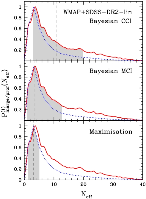
Figure 1: The 1D marginal (red/solid) and profile (blue/dotted) posteriors with respect to $N_{\rm eff}$ for our minimal model, the data set WMAP+SDSS-DR2-lin and top hat prior $0.2\leq h\leq 2.0$. The shaded regions are, from top to bottom, the Bayesian 68% central credible interval, the 68% minimum credible interval, and the $1\sigma$ interval derived from maximisation. The dashed vertical lines mark, from top to bottom, the posterior mean $\langle N_{\rm eff}\rangle$, the 1D marginal posterior mode $\hat{N}_{\rm eff}^{(1)}$, and the global best fit $\hat{N}_{\rm eff}$.

5.4 Marginalisation of the posterior

For multi-parameter models typically encountered in cosmology, the information carried by the multi-dimensional hypersurface $\partial A_{\gamma}$ is often not useful in practice and must be “compressed.” It is common to map the posterior probability $P({\bm{\theta}}|{\bm{x}})$ onto a lower-dimensional subspace by the process of marginalisation,

$$P^{(n)}_{\rm marge}({\bm{\theta}}^{(n)})\propto\int d\theta_{n+1}\ldots d\theta_{N}\ P({\bm{\theta}}|{\bm{x}}),$$ (5.5)

where ${\bm{\theta}}^{(n)}=(\theta_{1},\dots,\theta_{n})$ represents the parameters in the $n$-dimensional subspace. Point estimates for ${\bm{\theta}}^{(n)}$ and credible regions may then be constructed from the marginal posterior probability in analogy to section 5.3 above.

Marginalisation favours regions of parameter space that contain a large volume of the probability density in the marginalised directions. This “volume effect” can sometimes lead to counter-intuitive results, such as suppression of the probability density for the global best fit parameters $\hat{\bm{\theta}}$ if they appear within sharp peaks or ridges that contain little volume. Moreover, the concept of volume itself depends on the choice of parameters. For example, a flat prior on a parameter or one on its logarithm have completely different effects on the volume in that parameter direction. Therefore, other methods of mapping the multi-dimensional posterior onto a lower-dimensional space can be useful.

5.5 Maximisation of the posterior

A complementary approach to marginalisation is to project $P({\bm{\theta}}|{\bm{x}})$ onto the $n$-dimensional subspace ${\bm{\theta}}^{(n)}$ by maximising along the remaining directions,

$$P^{(n)}_{\rm prof}({\bm{\theta}}^{(n)})\propto\max_{\theta_{n+1},\ldots,\theta_{N}}P({\bm{\theta}}|{\bm{x}}).$$ (5.6)

The resulting $n$-dimensional profile posterior $P^{(n)}_{\rm prof}({\bm{\theta}}^{(n)})$ has the advantage of preserving the true peak of the original $N$-dimensional posterior probability and hence the global best fit $\hat{\bm{\theta}}$. Figure 1 shows a realistic example of a 1D marginal and a 1D profile posterior in juxtaposition.

In addition, we introduce an effective chi-square measure for the goodness-of-fit relative to the global best fit,

$$\Delta\chi^{2}_{\rm eff}({\bm{\theta}}^{(n)})\equiv-2\ln\left[\frac{P^{(n)}_{\rm prof}({\bm{\theta}}^{(n)})}{P(\hat{\bm{\theta}}|{\bm{x}})}\right].$$ (5.7)

For $n=1$, we define loosely the “$1\sigma$” and “$2\sigma$” intervals as the 1D regions satisfying respectively $\Delta\chi^{2}_{\rm eff}\leq 1$ and $\Delta\chi^{2}_{\rm eff}\leq 4$. We emphasise that these intervals have no formal probabilistic interpretation. However, they do provide a raw assessment, unplagued by volume effects, of how well a given parameter value agrees with the data relative to the global best fit, and have the virtue of being invariant under reparameterisation of the model. Of course, if $P^{(1)}_{\rm prof/marge}(\theta)$ is Gaussian, then the $1\sigma$ and $2\sigma$ intervals thus derived coincide with the 1D marginal 68% and 95% minimum and central credible regions [42]. Maximisation was used in some recent studies of cosmological $N_{\rm eff}$ inference [7, 8, 10, 11, 12].

For simplicity our maximisation intervals are extracted from the same MCMC chains used to construct the Bayesian credible intervals. However, we caution that MCMC techniques are strictly speaking not designed for this purpose; there exist sophisticated optimisation methods such as simulated annealing that are much better suited to the task.

The bottom panel of figure 1 shows a realistic example of a one-dimensional $1\sigma$ interval constructed according to equation (5.7). For a very non-Gaussian situation such as depicted in this figure, the point estimates and corresponding credible intervals derived by the methods discussed here are very different.

6 Constraints in the minimal model

6.1 Numerical results

To study the impact of different statistical methodologies and of different combinations of data sets, we use the minimal model (i.e., vanilla+$N_{\rm eff}$) as a benchmark case. Each entry in table 6.1 gives a point estimate and the lower and upper ends of the appropriate 68% and 95% credible intervals for $N_{\rm eff}$. The first column indicates the combinations of cosmological data sets. To illustrate the strong degeneracy between $N_{\rm eff}$ and the Hubble parameter $h$ in some data sets and its consequences, we have used two different top-hat priors: the loose prior 1 ($0.2\leq h\leq 2.0$) and the more constraining prior 2 ($0.4\leq h\leq 1.0$).

In the columns showing the Bayesian central credible interval, we use the posterior mean $\langle N_{\rm eff}\rangle$ as a point estimate, which is the default output of GetDist. The Bayesian minimum credible interval is derived from the 1D marginal posterior probability distribution for $N_{\rm eff}$ and the corresponding point estimate is the 1D marginal posterior mode $\hat{N}_{\rm eff}^{(1)}$. In the case of maximisation, the point estimate is the global best fit $\hat{N}_{\rm eff}$. Here, the associated intervals are the effective $1\sigma$ and $2\sigma$ regions defined by equation (5.7).

Table 2: Point estimates and credible intervals (68% and 95%) for $N_{\rm eff}$ in our minimal model “vanilla+$N_{\rm eff}$”. The priors for the free parameters are given in table 1. Priors 1 and 2 differ only for the Hubble parameter. We consider also two large combinations of data sets, All-lin = WMAP+BAO+SNIa+LSS-lin and All-Q = WMAP+BAO+SNIa+LSS-Q.

Bayesian CCI Bayesian MCI Maximisation $\langle N_{\rm eff}\rangle^{~{}68\%\uparrow,~{}95\%\uparrow}_{~{}68\%\downarrow,~{}95\%\downarrow}$ $\hat{N}_{\rm eff}^{(1)}\vphantom{\hat{N}_{\rm eff}}{}^{~{}68\%\uparrow,~{}95\%\uparrow}_{~{}68\%\downarrow,~{}95\%\downarrow}$ $\hat{N}_{\rm eff}\vphantom{\hat{N}_{\rm eff}}^{~{}1\sigma\uparrow,~{}2\sigma\uparrow}{}_{~{}1\sigma\downarrow,~{}2\sigma\downarrow}$ Data Prior 1 Prior 2 Prior 1 Prior 2 Prior 1 Prior 2 WMAP $22^{~{}37,~{}46}_{~{}7.3,~{}2.6}$ $5.8^{~{}8.8,~{}11}_{~{}3.0,~{}1.5}$ $6.8^{~{}32,~{}45}_{~{}2.8,~{}1.5}$ $4.2^{~{}7.9,~{}11}_{~{}2.2,~{}1.2}$ $3.9^{~{}6.1,~{}27}_{~{}1.5,~{}0.6}$ $3.9^{~{}6.1,~{}12}_{~{}1.5,~{}0.6}$ +SDSS-DR2-Q $14^{~{}26,~{}37}_{~{}3.6,~{}1.2}$ $4.8^{~{}7.7,~{}10}_{~{}2.1,~{}1.0}$ $3.6^{~{}18,~{}34}_{~{}0.6,~{}0.0}$ $3.7^{~{}6.4,~{}9.7}_{~{}1.1,~{}0.7}$ $2.6^{~{}5.6,~{}14}_{~{}1.0,~{}0.3}$ $2.3^{~{}5.6,~{}11}_{~{}1.0,~{}0.6}$ +SDSS-DR2-lin $11^{~{}20,~{}32}_{~{}3.0,~{}1.2}$ $4.9^{~{}8.0,~{}10}_{~{}2.0,~{}0.7}$ $3.6^{~{}13,~{}28}_{~{}0.7,~{}0.3}$ $4.3^{~{}6.5,~{}9.9}_{~{}0.9,~{}0.5}$ $3.2^{~{}5.1,~{}12}_{~{}1.2,~{}0.2}$ $3.2^{~{}5.1,~{}11}_{~{}1.3,~{}0.2}$ +2dF-Q $3.2^{~{}5.2,~{}8.4}_{~{}1.1,~{}0.3}$ $2.6^{~{}4.3,~{}5.7}_{~{}1.1,~{}0.4}$ $1.6^{~{}4.2,~{}7.5}_{~{}0.4,~{}0.0}$ $1.4^{~{}3.9,~{}5.5}_{~{}0.7,~{}0.0}$ $1.5^{~{}2.4,~{}5.3}_{~{}0.6,~{}-}$ $1.5^{~{}2.4,~{}5.0}_{~{}0.6,~{}-}$ +2dF-lin $4.6^{~{}7.1,~{}10}_{~{}2.2,~{}1.1}$ $4.4^{~{}6.8,~{}9.6}_{~{}2.1,~{}1.1}$ $2.9^{~{}5.8,~{}9.5}_{~{}1.3,~{}0.6}$ $3.2^{~{}5.7,~{}9.4}_{~{}1.4,~{}0.7}$ $2.6^{~{}4.5,~{}7.9}_{~{}1.2,~{}0.6}$ $2.6^{~{}4.5,~{}7.9}_{~{}1.2,~{}0.6}$ +SDSS-LRG-Q $3.5^{~{}5.1,~{}7.4}_{~{}2.0,~{}1.1}$ $3.5^{~{}5.1,~{}7.4}_{~{}2.0,~{}1.1}$ $2.6^{~{}4.5,~{}6.9}_{~{}1.5,~{}0.8}$ $2.5^{~{}4.5,~{}6.9}_{~{}1.5,~{}0.8}$ $2.7^{~{}4.1,~{}6.3}_{~{}1.5,~{}0.8}$ $2.7^{~{}4.1,~{}6.3}_{~{}1.5,~{}0.8}$ +SDSS-LRG-lin $4.0^{~{}5.8,~{}9.4}_{~{}2.1,~{}1.2}$ $3.5^{~{}5.0,~{}6.6}_{~{}2.1,~{}1.3}$ $2.6^{~{}4.9,~{}8.4}_{~{}1.5,~{}0.7}$ $2.8^{~{}4.6,~{}6.3}_{~{}1.8,~{}1.1}$ $2.7^{~{}4.3,~{}6.2}_{~{}1.8,~{}0.8}$ $2.7^{~{}4.0,~{}6.2}_{~{}1.8,~{}1.2}$ +BAO $3.5^{~{}5.0,~{}6.8}_{~{}2.1,~{}1.1}$ $3.5^{~{}5.0,~{}6.8}_{~{}2.1,~{}1.1}$ $2.8^{~{}4.7,~{}6.4}_{~{}1.8,~{}0.8}$ $2.8^{~{}4.7,~{}6.4}_{~{}1.8,~{}0.8}$ $2.1^{~{}4.7,~{}6.6}_{~{}1.4,~{}0.9}$ $2.1^{~{}4.7,~{}6.6}_{~{}1.4,~{}0.9}$ +SNIa $20^{~{}34,~{}44}_{~{}6.4,~{}2.3}$ $5.9^{~{}9.1,~{}11}_{~{}2.8,~{}0.9}$ $4.3^{~{}28,~{}42}_{~{}2.8,~{}0.4}$ $4.1^{~{}8.7,~{}11}_{~{}2.4,~{}0.9}$ $3.6^{~{}6.3,~{}24}_{~{}1.4,~{}0.3}$ $3.6^{~{}6.3,~{}12}_{~{}1.6,~{}0.3}$ +HST $3.9^{~{}5.7,~{}8.3}_{~{}2.1,~{}1.2}$ $4.0^{~{}5.7,~{}7.5}_{~{}2.4,~{}1.4}$ $3.3^{~{}5.1,~{}7.7}_{~{}1.6,~{}0.8}$ $3.6^{~{}5.3,~{}7.0}_{~{}2.1,~{}1.0}$ $2.9^{~{}4.6,~{}7.6}_{~{}1.6,~{}0.4}$ $2.9^{~{}4.5,~{}6.4}_{~{}1.6,~{}0.9}$ +Ly$\alpha$ $7.6^{~{}10,~{}13}_{~{}5.2,~{}3.6}$ $6.9^{~{}9.0,~{}11}_{~{}4.9,~{}3.5}$ $6.8^{~{}9.3,~{}12}_{~{}4.6,~{}3.3}$ $6.4^{~{}8.8,~{}11}_{~{}4.6,~{}3.2}$ $6.6^{~{}8.0,~{}12}_{~{}4.9,~{}3.3}$ $6.6^{~{}7.7,~{}10}_{~{}5.3,~{}3.3}$ All-lin — $2.9^{~{}4.0,~{}5.3}_{~{}1.8,~{}1.1}$ — $2.6^{~{}3.7,~{}5.1}_{~{}1.5,~{}0.9}$ — $2.7^{~{}3.3,~{}5.0}_{~{}1.5,~{}0.8}$ All-lin+HST — $2.8^{~{}3.7,~{}4.9}_{~{}1.9,~{}1.3}$ — $2.6^{~{}3.6,~{}4.8}_{~{}1.8,~{}1.1}$ — $2.7^{~{}3.2,~{}4.5}_{~{}2.0,~{}1.1}$ All-Q — $2.3^{~{}3.2,~{}4.4}_{~{}1.4,~{}0.7}$ — $2.0^{~{}3.1,~{}4.1}_{~{}1.2,~{}0.5}$ — $2.0^{~{}2.4,~{}4.0}_{~{}1.3,~{}0.6}$ All-Q+HST — $2.5^{~{}3.5,~{}4.3}_{~{}1.6,~{}1.0}$ — $2.4^{~{}3.3,~{}4.3}_{~{}1.6,~{}0.9}$ — $2.2^{~{}2.7,~{}3.8}_{~{}1.6,~{}0.9}$ All-Q+Ly$\alpha$ — $4.4^{~{}5.5,~{}6.9}_{~{}3.3,~{}2.4}$ — $4.4^{~{}5.4,~{}6.6}_{~{}3.2,~{}2.3}$ — $4.2^{~{}4.7,~{}6.4}_{~{}3.4,~{}2.4}$ All-Q+Ly$\alpha$+HST — $3.9^{~{}4.8,~{}5.9}_{~{}3.0,~{}2.3}$ — $3.8^{~{}4.7,~{}5.8}_{~{}2.9,~{}2.2}$ — $4.0^{~{}4.3,~{}5.6}_{~{}3.1,~{}2.3}$

6.2 Interpretation of statistics

To compare estimates from different inference schemes, consider first the top half of table 6.1. The posterior mean and the CCI, i.e., the default output of GetDist, show a preference for large $N_{\rm eff}$ for almost all combinations of probes. The combinations WMAP, WMAP+SDSS-DR2, and WMAP+SNIa, in particular, appear to disfavour the standard value $N_{\rm eff}=3.046$ at more than 68% (prior 1). However, any evidence for $N_{\rm eff}>3.046$ disappears as soon as we impose the tighter prior 2 on $h$. This trend stems from the $N_{\rm eff}$-$h$-degeneracy which leads to a long tail of high $N_{\rm eff}$ in the 1D marginal posterior (figure 1). The tail in turn pushes the posterior mean and the CCI to larger $N_{\rm eff}$ values. Imposing a tighter prior on $h$ suppresses the tail and reduces this effect. In contrast, the 1D marginal posterior mode $\hat{N}_{\rm eff}^{(1)}$ and the global best fit $\hat{N}_{\rm eff}$ pick out the parameters with the highest probability densities, and turn out to be insensitive to the choice of $h$ prior. The tail region still has a strong impact on the upper MCI limits, but the lower limits are relatively unaffected. The $N_{\rm eff}$ constraints from WMAP in table 6.1 provide an excellent illustration of this point. The $1\sigma$ and $2\sigma$ intervals from maximisation depend even less on the $h$ prior, since this construction makes no reference to the volume of the posterior and is therefore insensitive to tail regions once the 1D profile posterior drops below $e^{-2}$ relative to the peak. As argued earlier (section 5.3), in Bayesian inference only the MCI provides a meaningful answer to the question, what are the most probable values of $N_{\rm eff}$ implied by the data. Our explicit examples show that inference based on the CCI, the default output of GetDist, can lead to incorrect conclusions.

6.3 Scale-dependent bias

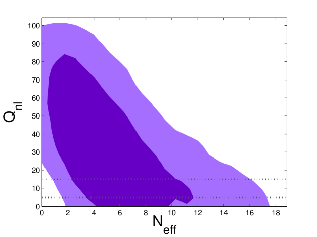
Turning to the issue of bias in the galaxy power spectrum, we see in table 6.1 that the two different measures introduced in section 4 to bypass or account for the scale dependence, namely, using only linear data at $k<0.1\ h\ {\rm Mpc}^{-1}$, or adopting the bias correction formula (4.2), generally produce consistent results. The agreement between WMAP+SDSS-DR2-lin and WMAP+SDSS-DR2-Q, and between WMAP+SDSS-LRG-lin and WMAP+SDSS-LRG-Q are excellent, suggesting that the effects of scale-dependent biasing have been successfully ameliorated. The WMAP+2dF-lin and WMAP+2dF-Q results do show a slight discrepancy at roughly the 68% level. This can most likely be put down to statistical fluctuations, but recall that the bias correction formula (4.2) has not been tested for nonstandard cosmologies and its application here is, strictly speaking, experimental. The analyses of Seljak et al. [9] and Mangano et al. [13] found a very high $N_{\rm eff}=7.8^{~{}8.9,~{}10}_{~{}7.1,~{}4.6}$ for WMAP+SDSS-DR2+SNIa, which can only be accommodated within our corresponding MCI estimates, $N_{\rm eff}=3.7^{~{}6.4,~{}9.7}_{~{}1.1,~{}0.7}$ for WMAP+SDSS-DR2-Q and $N_{\rm eff}=4.3^{~{}6.5,~{}9.9}_{~{}0.9,~{}0.5}$ for WMAP+SDSS-DR2-lin, at more than the 68% level. Both groups used the bias correction formula (4.2), but adopted the Gaussian prior $Q_{\rm nl}=10\pm 5$, a range supposedly determined from numerical simulations, although no source is cited. As a test, we have performed a fit of WMAP+SDSS-DR2-Q+SNIa using the same Gaussian prior on $Q_{\rm nl}$. We find $N_{\rm eff}=6.2^{~{}10,~{}12}_{~{}4.1,~{}1.9}$ (MCI) and $N_{\rm eff}=7.0^{~{}9.9,~{}12}_{~{}4.1,~{}2.2}$ (CCI), which include the high $N_{\rm eff}$ values of Refs. [9, 13] in the 68% region. Excluding SNIa from the fit yields essentially the same constraints. These test results clearly indicate that the choice of $Q_{\rm nl}$ prior plays an important role in the inference of $N_{\rm eff}$. In this case, the choice of $Q_{\rm nl}=10\pm 5$ tends to push the preferred $N_{\rm eff}$ to higher values. We are not able to reproduce the very tight error bars for $N_{\rm eff}$ reported in Refs. [9, 13], which may be due to different priors assumed for the marginalised parameters, or because of a slightly larger $k_{\rm max}\sim 0.15\ h\ {\rm Mpc}^{-1}$ adopted in these analyses. However, we also observe a peculiar feature in their credible intervals: the 68% interval is some three times smaller than the 95% interval. This suggests some highly non-Gaussian behaviour in their marginal posterior for $N_{\rm eff}$, because in a Gaussian distribution, the ratio of the intervals is $1:2$. Figure 2: The 2D marginal 68% and 95% allowed regions in the minimal model for $N_{\rm eff}$ and $Q_{\rm nl}$, using the data set WMAP+SDSS-DR2-Q+SNIa and prior 2. The horizontal dotted lines indicate the $1\sigma$ range of the Gaussian prior $Q_{\rm nl}=10\pm 5$. The dependence on the $Q_{\rm nl}$ prior traces its origin to a degeneracy between $N_{\rm eff}$ and $Q_{\rm nl}$. Figure 2 shows the 2D marginal 68% and 95% allowed regions in $N_{\rm eff}$-$Q_{\rm nl}$-space for the data set WMAP+SDSS-DR2-Q+SNIa. Evidently, imposing the restrictive prior $Q_{\rm nl}=10\pm 5$ cuts off much of the parameter space that favours low values of $N_{\rm eff}$. To our knowledge no simulation of mock galaxy catalogues involving a nonstandard $N_{\rm eff}$ value has ever been reported in the literature. Without the backing of simulations (or other independent input) there is no justification to impose a restrictive prior on $Q_{\rm nl}$ when performing a fit with $N_{\rm eff}$ as a free parameter. The best strategy in such circumstances is to use a broad and uniform prior on $Q_{\rm nl}$, as adopted in our analysis and also advocated in Ref. [1]. To summarise, we find that imposing a $Q_{\rm nl}=10\pm 5$ prior for the WMAP+SDSS-DR2-Q+SNIa fit biases the preferred $N_{\rm eff}$ to higher values. This may account for the difference between our result and those reported in Refs. [9, 13].

6.4 Combining all data sets

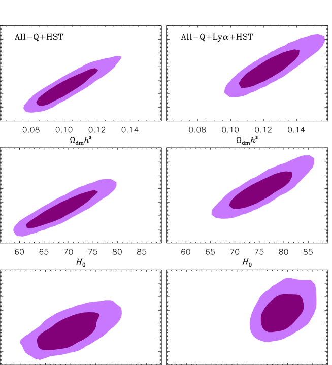
Having identified and corrected the problematic issues, we now turn to our own $N_{\rm eff}$ estimates. An inspection of table 6.1 reveals that, except for those sets including Ly$\alpha$, none of the combinations of probes shows any significant evidence for $N_{\rm eff}\neq 3.046$, a value that always sits comfortably within the 68% MCI. The combination of all linear data together with HST (All-lin+HST) gives $N_{\rm eff}=2.6^{~{}3.6,~{}4.8}_{~{}1.8,~{}1.1}$. Discarding HST leaves the best fit unchanged, but slightly loosens the credible intervals. Including nonlinear data in the galaxy power spectrum tends to reduce the numbers a little to $N_{\rm eff}=2.0^{~{}3.1,~{}4.1}_{~{}1.2,~{}0.5}$ (All-Q), essentially because 2dF-Q prefers a low $N_{\rm eff}$. Adding HST shifts it up again to $N_{\rm eff}=2.4^{~{}3.3,~{}4.3}_{~{}1.6,~{}0.9}$. We repeat that the bias correction formula (4.2) may not be applicable in nonstandard cosmologies so that numbers from the Q sets must be interpreted with caution. Another interesting feature is that, with the exception of WMAP+2dF-Q, all combinations of data sets prefer a nonzero $N_{\rm eff}$ at the 95% level or better. This is in contrast to the results of Ref. [12], which finds no lower 95% limit from the WMAP data alone. We have not investigated where the differences come from. As mentioned before, the WMAP+2dF-Q data set tends to prefer lower values of $N_{\rm eff}$ and as such produces no lower 95% limit on $N_{\rm eff}$. The Ly$\alpha$ data appear to be the only data set that prefers a much larger value of $N_{\rm eff}$, with WMAP+Ly$\alpha$ disfavouring $N_{\rm eff}=3.046$ at 95%. When combined with other data sets, however, the evidence against $N_{\rm eff}=3.046$ is weakened to the 68% level, $N_{\rm eff}=3.8^{~{}4.7,~{}5.8}_{~{}2.9,~{}2.2}$ for All-Q+Ly$\alpha$+HST, because 2dF-Q’s preference for small $N_{\rm eff}$ values tends to pull in the opposite direction. Figure 3: The 2D marginal 68% and 95% allowed regions in the minimal model for the indicated pairs of parameters. Plots in the left column use the All-Q+HST data set, while those in the right column include also Ly$\alpha$ (All-Q+Ly$\alpha$+HST). The origin of Ly$\alpha$’s preference for large values of $N_{\rm eff}$ can be gleaned from figure 3. The Ly$\alpha$ data prefer a much higher amplitude of density fluctuations at small scales, quantified by $\sigma_{8}$, than other data sets. This is particularly evident in the bottom panels of figure 3. The higher $\sigma_{8}$ value required by Ly$\alpha$ forces $N_{\rm eff}$ upwards and cuts away the allowed region for low $N_{\rm eff}$ values. As can be seen in the same figure, with the inclusion of Ly$\alpha$, the upper bound on $N_{\rm eff}$ comes mainly from the HST prior on $H_{0}$. Since $N_{\rm eff}$ and $H_{0}$ both control the epoch of matter–radiation equality and are thus strongly degenerate, a large $N_{\rm eff}$ can only be accommodated by a high value of $H_{0}$. However, such high values are strongly disfavoured by the HST data. The overall shift in the allowed range for $N_{\rm eff}$ between WMAP+Ly$\alpha$ and All-Q+Ly$\alpha$ also points to the fact that the SDSS-Ly$\alpha$ data is not completely compatible with other data sets (see, e.g., Refs. [9, 43]).

6.5 Towards Gaussianity

A striking feature in table 6.1 is that when all data sets are combined, the three different statistical methods give almost identical results. The reason is that the combination of CMB, LSS, and SNIa data effectively breaks all parameter degeneracies and yields a posterior distribution that is very close to Gaussian, a limit in which all three methods must give the same result. The lower half of table 6.1 nicely confirms this expectation.

7 Extended models

We now consider constraints on $N_{\rm eff}$ in the context of extended models that allow also for nonvanishing neutrino masses. As in the case of the minimal model, we calculate the bounds within a conservative approach using only linear data (All-lin), as well as a more speculative one that utilises the stronger, but more model-dependent All-Q data set. Since, as we saw in section 6, $N_{\rm eff}$ exhibits a strong degeneracy with the Hubble parameter $H_{0}$ in some data sets, we consider both options of including and excluding the HST data in our analysis. We do not use the Ly$\alpha$ data for the extended models. Table 3 shows our constraints on $N_{\rm eff}$ for four choices of extended models: vanilla+$N_{\rm eff}$ extended with $f_{\nu}$, $f_{\nu}$+$\alpha_{s}$+$w$, ${}^{3}f_{\nu}$, and ${}^{3}f_{\nu}$+$\alpha_{s}$+$w$. Table 3: Point estimates and credible intervals (68% and 95%) for $N_{\rm eff}$ in four extended model spaces. In the top segment, the minimal vanilla+$N_{\rm eff}$ model is extended with $f_{\nu}$ and $f_{\nu}$+$\alpha_{s}$+$w$ ($N_{m}=N_{\rm eff}$), while in the middle segment the extensions are ${}^{3}f_{\nu}$ and ${}^{3}f_{\nu}$+$\alpha_{s}$+$w$ ($N_{m}=3.046$) as defined in section 2. The bottom segment contains results for the minimal model copied from table 6.1. The priors for the free parameters are given in table 1. The columns headed “prior 2” use a top hat prior $0.4<h<1.0$, while those with “+HST” use in addition the HST result. The data sets used are All-lin = WMAP+BAO+SNIa+LSS-lin and All-Q = WMAP+BAO+SNIa+LSS-Q. Bayesian CCI Bayesian MCI Maximisation $\langle N_{\rm eff}\rangle^{~{}68\%\uparrow,~{}95\%\uparrow}_{~{}68\%\downarrow,~{}95\%\downarrow}$ $\hat{N}_{\rm eff}^{(1)}\vphantom{\hat{N}_{\rm eff}}{}^{~{}68\%\uparrow,~{}95\%\uparrow}_{~{}68\%\downarrow,~{}95\%\downarrow}$ $\hat{N}_{\rm eff}\vphantom{\hat{N}_{\rm eff}}^{~{}1\sigma\uparrow,~{}2\sigma\uparrow}{}_{~{}1\sigma\downarrow,~{}2\sigma\downarrow}$ Model Data Prior 2 +HST Prior 2 +HST Prior 2 +HST +$f_{\nu}$ All-lin $4.0^{~{}5.6,~{}8.2}_{~{}2.5,~{}1.5}$ $3.7^{~{}4.9,~{}6.3}_{~{}2.6,~{}1.8}$ $3.2^{~{}5.0,~{}7.8}_{~{}2.0,~{}1.1}$ $3.6^{~{}4.7,~{}6.1}_{~{}2.4,~{}1.6}$ $3.0^{~{}4.6,~{}6.2}_{~{}2.0,~{}1.1}$ $3.7^{~{}4.1,~{}5.7}_{~{}2.5,~{}1.8}$ +$f_{\nu}$ All-Q $3.6^{~{}5.0,~{}7.0}_{~{}2.2,~{}1.1}$ $3.5^{~{}4.5,~{}5.8}_{~{}2.4,~{}1.7}$ $2.9^{~{}4.7,~{}6.6}_{~{}1.9,~{}0.8}$ $3.2^{~{}4.3,~{}5.6}_{~{}2.2,~{}1.5}$ $3.2^{~{}3.8,~{}5.5}_{~{}2.1,~{}1.3}$ $3.0^{~{}3.8,~{}5.3}_{~{}2.3,~{}1.6}$ +$f_{\nu}$+$\alpha_{s}$+$w$ All-lin $3.7^{~{}5.3,~{}8.1}_{~{}2.0,~{}1.0}$ $3.7^{~{}5.1,~{}6.6}_{~{}2.3,~{}1.4}$ $3.1^{~{}4.9,~{}7.6}_{~{}1.6,~{}0.4}$ $2.6^{~{}4.7,~{}6.4}_{~{}2.0,~{}1.2}$ $2.5^{~{}3.2,~{}5.5}_{~{}1.5,~{}0.8}$ $3.0^{~{}3.6,~{}5.5}_{~{}2.3,~{}1.1}$ +$f_{\nu}$+$\alpha_{s}$+$w$ All-Q $3.3^{~{}4.9,~{}7.8}_{~{}1.8,~{}0.9}$ $3.3^{~{}4.6,~{}6.3}_{~{}1.9,~{}1.0}$ $2.3^{~{}4.2,~{}6.8}_{~{}1.3,~{}0.5}$ $3.0^{~{}4.3,~{}6.1}_{~{}1.7,~{}0.8}$ $2.6^{~{}3.0,~{}5.1}_{~{}1.5,~{}0.5}$ $2.9^{~{}4.2,~{}5.1}_{~{}1.7,~{}1.0}$ +${}^{3}f_{\nu}$ All-lin $4.9^{~{}5.3,~{}8.0}_{~{}3.0,~{}3.0}$ $4.4^{~{}4.8,~{}6.7}_{~{}3.0,~{}3.0}$ $3.2^{~{}5.3,~{}8.0}_{~{}3.0,~{}3.0}$ $3.2^{~{}4.8,~{}6.7}_{~{}3.0,~{}3.0}$ $3.0^{~{}3.8,~{}5.7}_{~{}3.0,~{}3.0}$ $3.0^{~{}3.9,~{}5.7}_{~{}3.0,~{}3.0}$ +${}^{3}f_{\nu}$ All-Q $4.4^{~{}4.6,~{}7.1}_{~{}3.0,~{}3.0}$ $4.2^{~{}4.5,~{}6.1}_{~{}3.0,~{}3.0}$ $3.0^{~{}4.6,~{}7.1}_{~{}3.0,~{}3.0}$ $3.2^{~{}4.5,~{}6.1}_{~{}3.0,~{}3.0}$ $3.0^{~{}3.9,~{}5.2}_{~{}3.0,~{}3.0}$ $3.0^{~{}3.7,~{}5.0}_{~{}3.0,~{}3.0}$ +${}^{3}f_{\nu}$+$\alpha_{s}$+$w$ All-lin $5.1^{~{}5.3,~{}9.4}_{~{}3.0,~{}3.0}$ $4.4^{~{}4.7,~{}6.7}_{~{}3.0,~{}3.0}$ $3.0^{~{}5.3,~{}9.4}_{~{}3.0,~{}3.0}$ $3.5^{~{}4.7,~{}6.7}_{~{}3.0,~{}3.0}$ $3.0^{~{}3.9,~{}6.4}_{~{}3.0,~{}3.0}$ $3.2^{~{}4.0,~{}6.0}_{~{}3.0,~{}3.0}$ +${}^{3}f_{\nu}$+$\alpha_{s}$+$w$ All-Q $4.4^{~{}4.7,~{}7.3}_{~{}3.0,~{}3.0}$ $4.1^{~{}4.3,~{}5.8}_{~{}3.0,~{}3.0}$ $3.0^{~{}4.7,~{}7.3}_{~{}3.0,~{}3.0}$ $3.2^{~{}4.3,~{}5.8}_{~{}3.0,~{}3.0}$ $3.0^{~{}3.7,~{}5.0}_{~{}3.0,~{}3.0}$ $3.0^{~{}3.8,~{}5.0}_{~{}3.0,~{}3.0}$ Minimal All-lin $2.9^{~{}4.0,~{}5.3}_{~{}1.8,~{}1.1}$ $2.8^{~{}3.7,~{}4.9}_{~{}1.9,~{}1.3}$ $2.6^{~{}3.7,~{}5.1}_{~{}1.5,~{}0.9}$ $2.6^{~{}3.6,~{}4.8}_{~{}1.8,~{}1.1}$ $2.7^{~{}3.3,~{}5.0}_{~{}1.5,~{}0.8}$ $2.7^{~{}3.2,~{}4.5}_{~{}2.0,~{}1.1}$ Minimal All-Q $2.3^{~{}3.2,~{}4.4}_{~{}1.4,~{}0.7}$ $2.5^{~{}3.5,~{}4.3}_{~{}1.6,~{}1.0}$ $2.0^{~{}3.1,~{}4.1}_{~{}1.2,~{}0.5}$ $2.4^{~{}3.3,~{}4.3}_{~{}1.6,~{}0.9}$ $2.0^{~{}2.4,~{}4.0}_{~{}1.3,~{}0.6}$ $2.2^{~{}2.7,~{}3.8}_{~{}1.6,~{}0.9}$

7.1 $N_{m}=N_{\rm eff}$

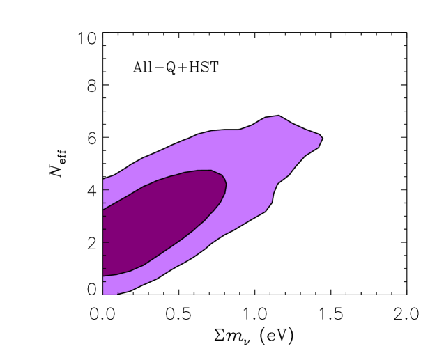
Consider first the top half of table 3. The two extended models have, respectively, vanilla+$N_{\rm eff}$+$f_{\nu}$ and vanilla+$N_{\rm eff}$+$f_{\nu}$+$\alpha_{s}$+$w$ as free parameters. Also in place is the condition $N_{m}=N_{\rm eff}$, meaning that all $N_{\rm eff}$ neutrinos have equal masses $m_{\nu}$. In both cases, it is evident that some new degeneracies have arisen with the introduction of additional free parameters; the marginal posteriors for $N_{\rm eff}$ are not perfect Gaussians for the All-lin and All-Q data sets, as indicated by the fact that their associated credible intervals from different constructions do not exactly overlap. However, none of the All-lin and All-Q results show any significant deviation from the standard $N_{\rm eff}=3.046$, and adding the HST data essentially serves to tighten the bounds. It is interesting to note that, in the case of the smaller vanilla+$N_{\rm eff}$+$f_{\nu}$ model, adding the HST data brings the marginal posterior for $N_{\rm eff}$ much closer to the Gaussian limit, so that the three different credible interval construction methods give almost identical results. Our best estimate is $N_{\rm eff}=3.2^{~{}4.3,~{}5.6}_{~{}2.2,~{}1.5}$ (All-Q+HST), values that are somewhat larger than those found in the minimal vanilla+$N_{\rm eff}$ model for the same data set, $N_{\rm eff}=2.4^{~{}3.3,~{}4.3}_{~{}1.6,~{}0.9}$, because of a degeneracy between $N_{\rm eff}$ and $f_{\nu}$. For the even larger vanilla+$N_{\rm eff}$+$f_{\nu}$+$\alpha_{s}$+$w$ model, an additional degeneracy between $N_{\rm eff}$ and $w$ comes into play so that the posterior for $N_{\rm eff}$ becomes more non-Gaussian. For All-Q+HST, for example, even though the MCI and the CCI have more or less converged (thus indicating a symmetric marginal posterior), the limits from maximisation are still very different. As our formal bound we use the MCI estimate for All-Q+HST, $N_{\rm eff}=3.0^{~{}4.3,~{}6.1}_{~{}1.7,~{}0.8}$, but also note that all three methods give credible intervals that are compatible with $N_{\rm eff}=3.046$ at better than 68%. Thus, as was the case for the minimal model, there is no evidence for any nonstandard value of $N_{\rm eff}$. Figure 4 shows the 2D marginal contours in the $\sum m_{\nu}$-$N_{\rm eff}$ plane for the extended model vanilla+$N_{\rm eff}$+$f_{\nu}$+$\alpha_{s}$+$w$ and the data set All-Q+HST. Some degeneracy persists between $\sum m_{\nu}$ and $N_{\rm eff}$, in contrast to earlier results from some of us [10]. The difference can be traced to a generally more conservative approach taken in the present work, particularly with regard to scale-dependent biasing, as well as a different statistical methodology (Bayesian marginalisation vs maximisation). Figure 4: The 2D marginal 68% and 95% allowed regions in $\sum m_{\nu}$ and $N_{\rm eff}$ in the extended model vanilla+$N_{\rm eff}$+$f_{\nu}$+$\alpha_{s}$+$w$, using the data set All-Q+HST. The corresponding contours for the model vanilla+$N_{\rm eff}$+${}^{3}f_{\nu}$+$\alpha_{s}$+$w$ are similar, but with a cut-off at $N_{\rm eff}=3$.

7.2 $N_{m}=3$

The bottom half of table 3 shows constraints on $N_{\rm eff}$ for essentially the same two classes of models, vanilla+$N_{\rm eff}$+${}^{3}f_{\nu}$ and vanilla+$N_{\rm eff}$+${}^{3}f_{\nu}$+$\alpha_{s}$+$w$, except we now impose the condition $N_{m}=3$, representing models with three massive neutrinos and $N_{\rm eff}-N_{m}$ massless species. This model is different from that presented above in section 7.1 because there is now a hard lower limit of $N_{\rm eff}=3$. The presence of a hard limit can in principle lead to some very disparate credible intervals from the three different construction methods. In the present case, however, the 1D marginal and profile posteriors for $N_{\rm eff}$ both peak at or very near the limit. It is therefore more useful to report, instead of a CCI, an upper 100$\gamma$% limit constructed by requiring that a fraction $\gamma$ of the marginal posterior’s volume lies to the left of the limit. This construction is also a default setting of GetDist for parameter estimation in the presence of hard limits. For simplicity, however, we shall continue to label an interval thus constructed as a CCI. The definitions of an MCI and a maximisation interval are the same as before. The fact that the marginal posterior for $N_{\rm eff}$ peaks at or very near the hard limit also means that, although the posterior mean and mode still differ, the CCI and the MCI will coincide, as is clearly shown in the bottom half of table 3. All estimates indicate that $N_{\rm eff}=3.046$ sits safely within the 68% region. Our best estimate for the smaller vanilla+$N_{\rm eff}$+${}^{3}f_{\nu}$ model, based on the MCI, is $N_{\rm eff}=3.2^{~{}4.5,~{}6.1}_{~{}3.0,~{}3.0}$ (All-Q+HST), while for the larger vanilla+$N_{\rm eff}$+${}^{3}f_{\nu}$+$\alpha_{s}$+$w$ model we find $N_{\rm eff}=3.2^{~{}4.3,~{}5.8}_{~{}3.0,~{}3.0}$ using the same data set.

8 Conclusions

Motivated by several recent, seemingly conflicting inferences of the cosmic radiation density (traditionally parameterised as the effective number of neutrino species $N_{\rm eff}$) from cosmological observations, we have re-examined the issue of cosmological $N_{\rm eff}$ determination in great detail and identified the reasons for the apparent discrepancies. Using a minimal model with $N_{\rm eff}$ as the only nonstandard parameter (i.e., vanilla+$N_{\rm eff}$), we find that the treatment of scale-dependent biasing in the galaxy power spectrum data is crucial to the derived value of $N_{\rm eff}$. The very high values of $N_{\rm eff}$ found in Refs. [9, 13] for the WMAP+SDSS-DR2+SNIa data and the same model can be traced to their treatment of the $Q_{\rm nl}$ parameter which quantifies the level of bias correction. The prior on $Q_{\rm nl}$ imposed in these studies, $Q_{\rm nl}=10\pm 5$, is significantly more restrictive than the parameter space allowed by the WMAP+SDSS-DR2-Q data. Because of a degeneracy between $N_{\rm eff}$ and $Q_{\rm nl}$, such a restrictive prior cuts out much of the parameter region that favours low values of $N_{\rm eff}$ and consequently biases the inferred $N_{\rm eff}$ towards high values (figure 2). The use of restrictive priors on $Q_{\rm nl}$ is unjustified when fitting nonstandard cosmologies, unless the priors have been verified/supplemented by simulations or other means under the same model assumptions. In the absence of such information, the best strategy is to use broad and uniform priors. When the WMAP measurements are combined with any other single data set (LSS, BAO, SNIa, or HST), we find that the inferred $N_{\rm eff}$ is always compatible with the standard value $N_{\rm eff}=3.046$ at 68% C.L. or better, except for the combination WMAP+Ly$\alpha$, which yields a high $N_{\rm eff}$ value in disagreement with 3.046 at more than 95%. The reason Ly$\alpha$ prefers a high $N_{\rm eff}$ originates in a well-known discrepancy in the inferred small-scale fluctuation amplitude between the SDSS-Ly$\alpha$ and the WMAP data. This can be understood from our figure 3. When all data sets (except Ly$\alpha$) are used in combination, we find tighter bounds on $N_{\rm eff}$ that are, again, compatible with $N_{\rm eff}=3.046$ at better than the 68% level. This finding is independent of whether we use galaxy power spectrum data only in the strictly linear regime or also at higher values of $k$, as long as scale-dependent bias is correctly taken into account. When Ly$\alpha$ is added to the fit, the inferred $N_{\rm eff}$ is again shifted to higher values because of Ly$\alpha$’s normalisation discrepancy with WMAP. As discussed in section 3.6 this discrepancy is most likely due to unaccounted systematics in the Ly$\alpha$ data. For this reason we quote a result without Ly$\alpha$, $N_{\rm eff}=2.6^{~{}3.6,~{}4.8}_{~{}1.8,~{}1.1}$, as our best current estimate of the constraints on $N_{\rm eff}$ in the minimal vanilla+$N_{\rm eff}$ model from WMAP+LSS-Q+BAO+SNIa+HST. Another very interesting point is that the statistical method used to construct credible intervals can have a strong impact on parameter inference when the posterior probability is non-Gaussian. Using an inappropriate interval construction can sometimes lead to incorrect inferences. This is especially true when fitting data sets that are not very constraining and therefore contain strong parameter degeneracies. However, when all available data sets are used in combination, they conspire to break each other’s degeneracies. The 1D posterior for $N_{\rm eff}$ in the minimal model approaches the Gaussian limit, and all three interval constructions used in our analysis, the Bayesian central and minimum credible intervals, and the non-Bayesian concept of maximisation, give almost identical results in this case. New parameter degeneracies arise when more free parameters are introduced in extended models. Even when the parameter inference is performed with all data sets combined, there is still some, albeit small, differences in the credible intervals obtained from the different methods. We have considered several different extended models in the present work, all including nonzero neutrino masses as a free parameter. While the formal constraints on $N_{\rm eff}$ differ slightly from model to model, we find again that $N_{\rm eff}=3.046$ is always compatible with data at the 68% C.L. or better, as long as we exclude the Ly$\alpha$ data. Because of the additional parameters the formal bounds on $N_{\rm eff}$ are somewhat relaxed relative to those derived for the minimal model. For our most general model (i.e., vanilla+$N_{\rm eff}$+$f_{\nu}$+$\alpha_{s}$+$w$, with $N_{\rm eff}$ equally massive neutrinos), we find $N_{\rm eff}=3.0^{~{}4.3,~{}6.1}_{~{}1.7,~{}0.8}$, based on the minimum credible interval, using the data set WMAP+LSS-Q+BAO+SNIa+HST. We consider also the case in which the total radiation density is split into three massive species and $N_{\rm eff}-3$ strictly massless ones. In this case we find almost identical upper bounds on $N_{\rm eff}$ as in the previous case with $N_{\rm eff}$ massive species (the lower bounds here are now always 3.0). Extra radiation density corresponding to at least one extra neutrino degree of freedom is allowed by all data sets at the 95% level. Thus, cosmological observations are not yet at a precision level sufficient to exclude very light sterile neutrinos, axions, majorons, or similar particles that were in thermal equilibrium after the QCD phase transition. With future CMB and weak gravitational lensing data this situation is set to change. For instance, with data from Planck and the future wide-field weak lensing survey LSST, a sensitivity of $\sigma(N_{\rm eff})\sim 0.07$ can be achieved [44]. Cosmology will then become an even more powerful probe of particle physics beyond the standard model.

Acknowledgements

We thank Anže Slosar for useful suggestions and comments on the manuscript. We acknowledge use of computing resources from the Danish Center for Scientific Computing (DCSC). In Garching and Munich, partial support by the Deutsche Forschungsgemeinschaft under the grant TR 27 “Neutrinos and beyond” and by the European Union under the ILIAS project, contract No. RII3-CT-2004-506222, is acknowledged.

References

References

http://lambda.gsfc.nasa.gov