Modified $p$-modes in penumbral filaments?

Abstract

Aims. The primary objective of this study is to search for and identify wave modes within a sunspot penumbra.

Methods. Infrared spectropolarimetric time series data are inverted using a model comprising two atmospheric components in each spatial pixel. Fourier phase difference analysis is performed on the line-of-sight velocities retrieved from both components to determine time delays between the velocity signals. In addition, the vertical separation between the signals in the two components is calculated from the Stokes velocity response functions.

Results. The inversion yields two atmospheric components, one permeated by a nearly horizontal magnetic field, the other with a less-inclined magnetic field. Time delays between the oscillations in the two components in the frequency range $2.5-4.5$ mHz are combined with speeds of atmospheric wave modes to determine wave travel distances. These are compared to expected path lengths obtained from response functions of the observed spectral lines in the different atmospheric components. Fast-mode (i.e., modified $p$-mode) waves exhibit the best agreement with the observations when propagating toward the sunspot at an angle $\sim$50° to the vertical.

1 Introduction

Disentangling the signatures of various atmospheric waves that are supported by structured magnetic atmospheres is a difficult, even daunting, task. Recent advances in dynamic, 2-D modeling of magnetised atmospheres (Rosenthal et al. 2002; Bogdan et al. 2003; Khomenko & Collados 2006), highlight the dilemma that observers face – i.e., measuring not just singular wave modes but the superposition of many magneto-atmospheric modes that most likely propagate in different directions and exist in differing plasma-$\beta$ environments. This poses a distinct problem, especially if studies do not resolve the true size scale of solar magnetic features.

However, information may be extracted from spatially unresolved structures by spectropolarimetry (e.g., the penumbral flux-tube work of Müller et al. 2002). This approach uses the full Stokes polarization spectra ($I$, $Q$, $U$, $V$), allowing physical properties of the emitting plasma to be inferred through the application of appropriate model atmospheres. The suitability of using Stokes profiles for wave diagnostics has been shown through numerical simulations (see, e.g., Solanki & Roberts 1992; Ploner & Solanki 1997, 1999), while Stokes profiles were also used by Rueedi et al. (1998) to interpret magnetic field oscillations in a sunspot as resulting from magneto-acoustic-gravity waves.

In this paper we present a method that may identify the form of wave which exists in a magnetic environment using the information available to full Stokes spectropolarimetry. The observational data, their reduction, and details of the form of atmospheric inversion procedure applied are outlined in Sect. 2. Results of response function calculations and a Fourier phase difference analysis are presented and discussed in Sect. 3 in terms of the various forms of wave modes which may exist at differing propagation angles, while in Sect. 4 the implications of our work are summarized.

Table 1: Atomic parameters of the observed lines. $\lambda_{0}$ denotes the laboratory wavelength, $\chi_{l}$ the excitation potential of the lower energy level, and $\log gf$ the logarithm of the oscillator strength times the multiplicity of the level. The parameters $\alpha$ and $\sigma$ (in units of the Bohr radius, $a_{0}$) are used to calculate the line broadening by collisions with neutral hydrogen, atoms, while $g_{l}$, $g_{u}$, and $\bar{g}$ are the calculated Landé factors of the lower and upper levels, and the effective value, respectively.

Species	$\lambda_{0}$	Configuration	$\chi_{l}$	$\log gf$	$\alpha$	$\sigma$	$g_{l}$	$g_{u}$	$\bar{g}$
	(Å)		(eV)	(dex)		($a_{0}$)
Fe i	15662.018	${}^{5}F_{5}-^{5}F_{4}$	5.83	0.19	0.24	1200	1.40	1.35	1.50
Fe i	15665.245	${}^{5}F_{1}-^{5}D_{1}$	5.98	-0.42	0.23	1283	0.00	1.50	0.75

2 Observations

A small and ellipsoidal sunspot, NOAA 10436, was observed on 21 August 2003 using the Tenerife Infrared Polarimeter (Martínez Pillet et al. 1999) attached to the 0.7 m German solar Vacuum Tower Telescope in Tenerife, Canary Islands. A fast scan was performed over the whole sunspot to obtain a global picture, comprising 79 slit positions of 0$\aas@@fstack{\prime\prime}$35 width (each with a slit integration time of 7 s) incrementally stepped 0$\aas@@fstack{\prime\prime}$4, from which the continuum intensity image in Fig. 1 was constructed. The sunspot was located somewhat out of disk centre ($\theta=26.7$°, $\mu=\cos\theta\approx 0.9$) and a light bridge separated the two umbrae.

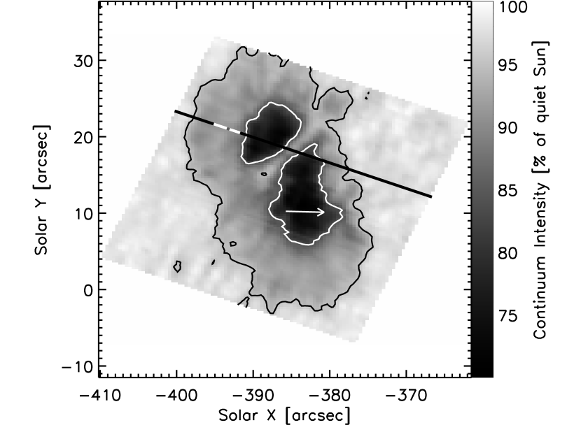
Figure 1: Continuum intensity image of NOAA 10436 at 15666.5$\pm$0.5 Å. White (black) contours mark the umbral/penumbral (penumbral/quiet Sun) boundaries. The straight black line marks the slit position during the time series and the white portion indicates the region studied in detail. The dark grey pixel within the white portion of the slit marks the position from which the profiles in Fig. 2 are taken, while the arrow in the umbra points to disk centre.

Prior to this scan, the slit was fixed across the sunspot and the full Stokes vector ($I$, $Q$, $U$, $V$) was measured (see Fig. 2 for example spectra) in a time series comprising 250 stationary-slit exposures acquired at a cadence of 14.75 s over 14:39-15:41 UT. Seeing conditions were moderate during the observations, with an estimated spatial resolution of around 1$\aas@@fstack{\prime\prime}$5. The most striking feature observed in the time series was the oscillatory behaviour of Stokes $Q$, most prominently seen in the inner part of the limb-side penumbra (white part of the slit in Fig. 1). This oscillation in the Stokes $Q$ signal is diplayed in Figs. 3c and 3d, where a dominant 5 min period is observed.

2.1 Spectral Lines

The recorded spectral region contains two moderately magnetically sensitive neutral iron lines (Fe i 15662.0 Å with effective Landé factor $\bar{g}=1.50$ and Fe i 15665.2 Å with $\bar{g}=0.75$) at a wavelength sampling of 29.7 mÅ pixel^-1. The data reduction included polarization demodulation and calibration, flat fielding, dark current and continuum correction, and the removal of instrumental cross-talk between the Stokes profiles (Collados 2003). The noise in the reduced data lay below $5\times 10^{-4}$ in units of continuum intensity. The wavelength calibration was done assuming that the core position of average quiet-Sun intensity profiles corresponds to the laboratory wavelength, $\lambda_{0}$, shifted towards the blue by 500 m s^-1, the approximate value for the blueshift in these lines deduced from the convective velocity relation of Nadeau (1988).

Table 1 presents the atomic data for the spectral lines used in this work, where laboratory wavelengths, electronic configurations, and excitation potentials were taken from Nave et al. (1994) while the parameters $\alpha$ and $\sigma$, which are used in the calculation of spectral line broadening by collisions with neutral perturbers, were taken from Anstee & O’Mara (1995, sp transitions). The two-component model of the quiet Sun from Borrero & Bellot Rubio (2002) was used to calculate empirical oscillator strengths for the observed lines, as in Borrero et al. (2003). For the 15665 Å line, the value for the derived oscillator strength is especially inaccurate (we estimate $\pm$0.2 dex) as the intensity profile is blended and the effective quantum number for the upper level was beyond the value given in the tables of Anstee & O’Mara (1995); here we take the maximum value provided by these authors to avoid large extrapolations.

Figure 2: Example penumbral profiles of Stokes $I$ (a), Stokes $Q$ (b), Stokes $U$ (c), and Stokes $V$ (d), each normalized to the local continnum intensity, $I_{C}$, from the pixel marked dark grey inside the region of interest shown in Fig. 1. Wavelengths are relative to the 15662 Å line, with dotted lines at the blueshift-corrected laboratory values.

Figure 2 represents an example of the observed penumbral profiles, in this case from the dark grey pixel inside the region of interest of Fig. 1. As already mentioned, the intensity profile of the 15665 Å line is blended with an unidentified profile. We identify the blend as solar – it varys in strength between quiet Sun and umbra – but its origin could not be determined. However, it seems that it is not magnetically sensitive because even when the field is strong, as in the penumbra, no residual polarization signal appears at that wavelength. In our analysis we only weakly consider the $I$ spectrum for this line but make full use of the polarization spectra ($Q$, $U$, $V$) because, although small in magnitude, they provide additional information.

The circular polarization (Stokes $V$) shows that the magnetic field points downward in the spot but, more interestingly, the linear polarization signals (Stokes $Q$ and $U$) are oppositely signed in each line. This is due to their opposite Zeeman patterns and can be easily proved following Landi degl’Innocenti (1992). In the weak magnetic field limit, it can be written that,

$$Q\left(\lambda_{0}\right)=-\frac{1}{4}\left(\bar{g}^{2}+\epsilon\right)\lambda_{B}^{2}\sin^{2}\gamma\cos 2\chi\left(\frac{\partial^{2}I_{0}}{\partial\lambda^{2}}\right)_{\lambda=\lambda_{0}}\ ,$$ (1)

$$U\left(\lambda_{0}\right)=-\frac{1}{4}\left(\bar{g}^{2}+\epsilon\right)\lambda_{B}^{2}\sin^{2}\gamma\sin 2\chi\left(\frac{\partial^{2}I_{0}}{\partial\lambda^{2}}\right)_{\lambda=\lambda_{0}}\ ,$$ (2)

where $\gamma$ is the inclination of the magnetic field vector to the line-of-sight (LOS), $\chi$ is the azimuthal angle of the magnetic field vector in the plane perpendicular to the LOS, $\lambda_{B}$ is the Zeeman wavelength splitting, $\bar{g}$ is the effective Landé factor of the transition, and $\epsilon$ is a correction factor for anomalous Zeeman triplets ($J_{L}\neq 0$ or $J_{U}\neq 1$ or $g_{L}\neq g_{U}$) given by,

$$\epsilon = \frac{1}{80}(7\left[J_{U}\left(J_{U}+1\right)-J_{L}\left(J_{L}+1\right)\right]^{2}$$ (3)

$$\ \ -16\left[J_{U}\left(J_{U}+1\right)+J_{L}\left(J_{L}+1\right)\right]+4)\left(g_{U}-g_{L}\right)^{2}\ ,$$

where $J_{L}$ and $J_{U}$ are the total angular momentum quantum numbers for the lower and upper transitions, respectively, as defined by the electronic configurations (Table 1), while $g_{L}$ and $g_{U}$ are the Landé factors of the lower and upper levels whose expressions can be analytically determined as these lines are in pure L-S coupling (see, e.g., del Toro Iniesta 2003). Values of $\bar{g}+\epsilon$ can be calculated, yielding $\simeq$2.2 for Fe i 15662 Å and $\simeq$$-1.1$ for Fe i 15665 Å, explaining the opposite linear polarization signals observed in Fig. 2. Note, the inversion technique detailed in the following section makes use of the full Zeeman splitting pattern and does not use the effective Landé factor.

2.2 Atmospheric Inversion

The data were inverted using the SPINOR inversion code (Frutiger 2000; Frutiger et al. 2000). Prior to the inversion we computed the relative Stokes $V$ area asymmetry (Borrero et al. 2004), defined as,

$$\delta A=\frac{\int V\left(\lambda\right)d\lambda}{\int|V\left(\lambda\right)|d\lambda}\ .$$ (4)

Given the small magnitude of $\delta A$ observed in the circular polarization over the inner limb-side penumbra (Fig. 3b; area between the dot-dashed lines) it is likely that these lines are not affected by strong gradients in either the magnetic field vector or velocity along the LOS. Therefore, we have adopted the same model as used by Borrero et al. (2004) and referred to as a two-component (2-C) inversion. This model consists of two magnetic components and one non-magnetic straylight component – all parameters except temperature are height independent in each component. The inversion returns the thermodynamic, magnetic, and kinematic structure of the atmosphere that provides the best fit to the observed Stokes ($I$, $Q$, $U$, $V$) polarization signals.

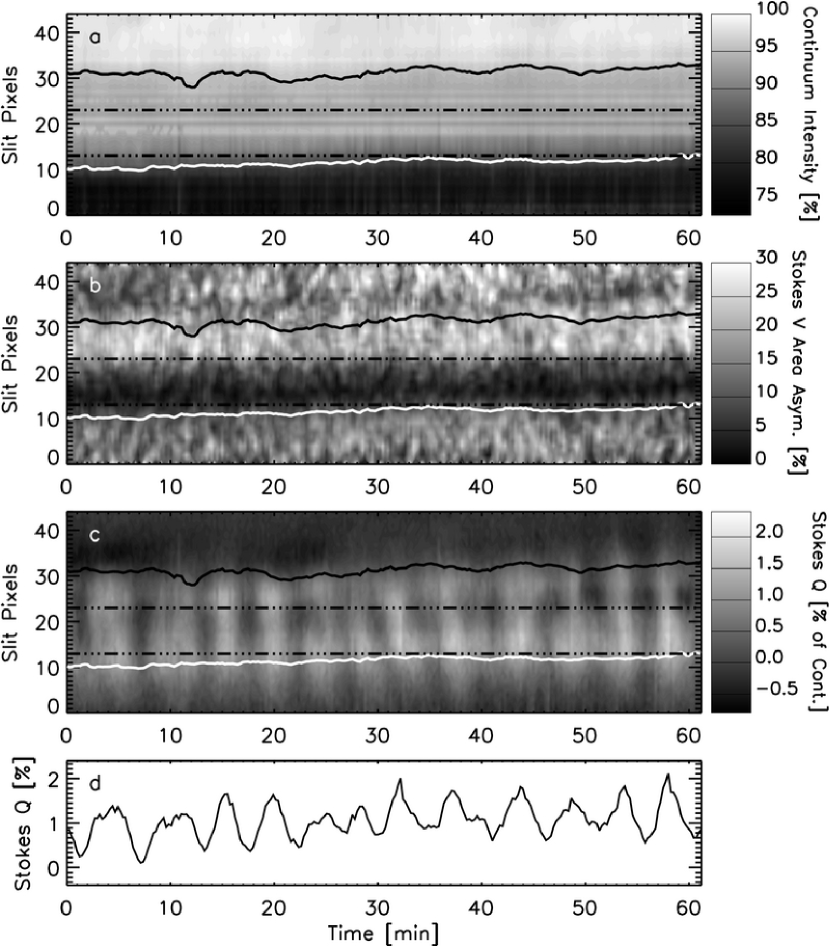
Figure 3: Space-time plots of continuum intensity as a percentage of average quiet-Sun continnum (a), magnitude of the relative Stokes $V$ area asymmetry (b), and Stokes $Q$ at +0.145 Å from the core of the 15662 Å line (c). d): Spatially-averaged Stokes $Q$ signal from the region of interest. Only the slit portion extending toward solar north east from the northern umbra is shown in a-c. The white (black) contour marks the umbral/penumbral (penumbral/quiet Sun) boundary and the dot-dashed lines bound the region studied (white area of slit in Fig.1).

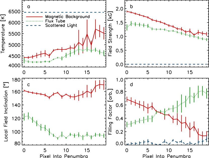
Figure 4: Variation through the limb-side penumbra of the parameters obtained by the inversion at $\log\left(\tau\right)=0$ : temperature (a), field strength (b), local solar inclination (c), and filling factor (d). Points mark the temporal mean for each spatial pixel and error bars extend over $\pm$1$\sigma$.

Parameters retrieved from the inner limb-side penumbra (Fig. 4; pixels $1-11$) yield a magnetic geometry consisting of a near-horizontal component, at local solar inclinations $\gamma^{\prime}\approx 90-125$° ($55-90$° from vertical), and a closer-to-vertical one, $\gamma^{\prime}\approx 150-160$° ($20-30$° from vertical), consistent with the observations of Title et al. (1993). Note that the retrieved values of $\gamma^{\prime}$, temperature, field strength, and filling factor are similar to those obtained by Borrero et al. (2004). From this point on, the near-horizontal component will be referred to as flux tube (FT) and the less-inclined one as magnetic background (MB) following the flux tube interpretation of Solanki & Montavon (1993), Schlichenmaier et al. (1998), Müller et al. (2002), and Borrero et al. (2005, 2006). Note that this interpretation is subject to current discussion (Spruit & Scharmer 2006). In principle, it may be possible to distinguish between the two scenarios by means of an analysis similar to ours, but this requires further development of the Spruit and Scharmer scenario and is beyond the scope of the current paper.

3 Results & Discussion

3.1 Height Separations

In the following analysis the height at which the oscillations are observed in both components plays an important role, so that we describe in detail how this height is determined. We compute the line depression response function (RF), which is most appropriate for the Stokes parameters (Grossmann-Doerth et al. 1988). The wavelength-integrated RFs of Stokes $Q$ to LOS velocity are presented in Fig. 5a since the velocity variations were most strongly observed in Stokes $Q$ (Fig. 3). The RFs for each of the components overlap over most of the atmosphere, but their center-of-gravity (COG), displayed as vertical lines, reveal a distinct separation between the components. These COG heights were taken as the origin of the LOS velocity signals.

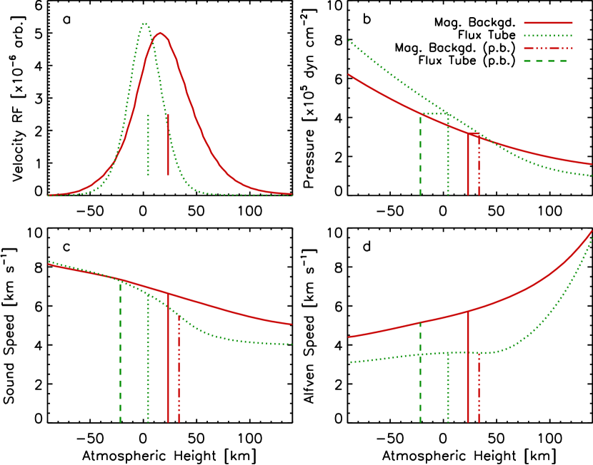
Figure 5: Height variation of wavelength-integrated 15662 Å and 15665 Å Stokes $Q$ velocity response (a), total pressure (b), acoustic (c), and Alfvénic (d) wave speeds for the magnetic background and flux tube atmospheres (solid and dotted curves, respectively). Vertical lines in a mark the COG in each component; vertical dashed and dot-dashed lines in b-d show these heights translated into the reference frame of the other atmosphere by enforcing total pressure balance.

One problem with comparing these COG heights is that each refers to the height scale of the atmosphere in which the lines were computed. The atmospheres returned by the inversion each have their own height scale due to the different effective temperatures (Fig. 4a) yielding different pressure scale heights (Fig. 5b). As such, they cannot be simply reduced to a single height scale, since pressure balance between the two atmospheres can only be enforced at a single height at a time.

In order to determine vertical height separations between the COG heights of the two components this height scale inequality must be overcome. This was achieved by enforcing total pressure balance between the two atmospheres at the COG heights. For example, in Fig. 5b the value from the FT pressure curve at the FT COG (dotted vertical line) is translated onto the MB pressure curve, yielding its pressure-balanced COG in the MB reference frame (dashed line). Similarly, the value from the MB pressure curve at the MB COG (solid vertical line) is translated onto the FT pressure curve, providing its pressure-balanced COG in the FT reference frame (dot-dashed line).

Through this approach we arrive at representative heights for the velocity signals of the MB and FT atmospheres in the reference frames of either atmosphere. Values are determined for both cases as a consistency check for the method. This allows the vertical separation distances of the velocity signals to be calculated in either of the reference frames – in the MB (FT) atmosphere it is the distance between the solid and dashed (dotted and dot-dashed) vertical lines. These heights also allow the retrieval of characteristic wave propagation speeds from the output inversion atmospheres (e.g., Figs. 5c and 5d).

3.2 Time Series Analysis

All atmospheric parameters except velocity were found to be time independent within the error bars. Clear periodic LOS velocity variations were observed in both atmospheric components, prompting the application of Fourier phase difference analysis following Krijger et al. (2001). The analysis was performed between the MB and FT velocity signals of eleven pixels of the inner limb-side penumbra. The phase difference from one pixel is the frequency-dependent phase lag of the FT velocity signal with respect to the MB signal, while the coherence measures the quality of phase difference variation.

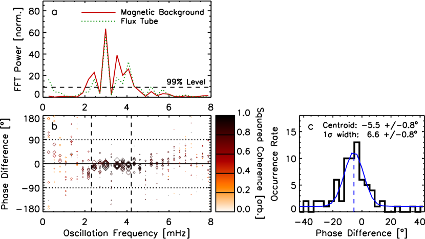
Figure 6: a): Fourier power spectra from co-spatial magnetic background and flux tube atmosphere LOS velocities (solid and dotted curves, respectively). b): Fourier phase difference spectra between the magnetic background and flux tube velocities from the eleven analyzed pixels. Darker shading denotes greater Fourier coherence and larger symbol size greater cross-spectral power. c): PDF of phase difference values over the range $2.5-4.5$ mHz. The thick curve displays the measured values and the thin curve the best-fit Gaussian profile to the data.

Figure 6 displays the output from applying such an analysis to the observed velocities. Example Fourier power spectra from one spatial pixel are given in Fig. 6a where both components obviously show power at very similar frequencies. The overplotted phase difference spectra for all eleven of the analyzed spatial pixels is presented in Fig. 6b, where symbol size represents the magnitude of cross-spectral power and shading denotes the coherence. Phase difference values are approximately constant in the range showing strongest cross-spectral power ($\sim$$2.5-4.5$ mHz) and, although close to zero, the probability distribution function (PDF) in Fig. 6c reveals that they are centred on $-5.5$°. This centroid phase difference value was converted to a time delay between the signals, resulting in values of $-6.3$ s to $-3.8$ s over the detected range of oscillation frequencies. Negative phase differences mean that the FT velocity leads the MB, agreeing with the COG heights in Fig. 5 for upward wave propagation.

3.3 Wave Modes

The range of atmospheric parameters existing in a sunspot penumbra supports the possibility of many differing forms of wave modes. However, all of these could be excited by $p$-mode waves propagating up towards the solar surface and the fact that the power peaks at $\sim$3 mHz (Fig. 6a) suggests that this is indeed the case for the observed wave modes. The dispersion relation for acoustic (i.e., $p$-mode) waves has the form $k^{2}c_{S}^{2}=\omega^{2}-\omega_{\rm{ac}}^{2}$, where $c_{S}$ is the sound speed, $\omega$ is the angular frequency, and $\omega_{\rm{ac}}$ is the acoustic cutoff frequency: waves are evanescent for $k^{2}<0$ and propagation occurs for $\omega>\omega_{\rm{ac}}$.

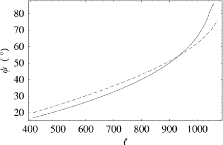
Figure 7: Variation of propagation angle from the vertical, $\psi$, with angular wave mode, $l$, for acoustic waves at a frequency of $3.5$ mHz. The solid curve shows the case 50 km below the equipartition level (where the acoustic and Alfvén speeds are equal) in a 1.75 kG field inclined at 20°, while the dashed curve is 90 km below the equipartition level in a 1.5 kG field inclined at 75° (the sampling heights and configurations of the magnetic background and flux tube components, respectively).

Table 2: Differences between COG values of RF-predicted and calculated path length distributions. Values are presented for cases of waves excited by $p$-modes with inclinations, $\psi$, of 0°, 40°, 50°, and 60° from the vertical. Note that in the case of vertical propagation ($\psi=0$°) there is no distiction between ingressing or egressing forms of fast-mode waves, hence only one value is provided. When sampling a low plasma-$\beta$ environment the Alfvén and slow-mode waves are field aligned, remaining invariant to changes in the originating $p$-mode inclination: values are not provided for these two wave modes in the flux-tube reference frame due to their large magnitude and obvious incorrectness.

Wave Mode	Absolute Separation of COG Values [km]
	$\psi=0$°		$\psi=40$°		$\psi=50$°		$\psi=60$°
	MB	FT	MB	FT	MB	FT	MB	FT
Alfvénic	5	…	5	…	5	…	5	…
Slow	9	…	9	…	9	…	9	…
Acoustic	7	12	2	6	8	1	20	7
Fast (ingressing)	10	16	5	9	0	4	12	5
Fast (egressing)	…	…	1	8	5	2	16	6

Attributing the observed phase differences in the $2.5-4.5$ mHz range to propagating waves conflicts with this simple picture of evanescent behaviour as the cutoff frequency at the photosphere is $\sim$5 mHz in the isothermal case. However, in the presence of a magnetic field the acoustic cutoff is reduced for non-vertical waves in a rather complicated manner (Bel & Leroy 1977). The largest deviation occurs for waves in the strong-field limit (i.e., when the Alfvén speed, $v_{A}$, is much greater than $c_{S}$). In this situation the cutoff frequency is lowered to $\omega_{\rm{ac}}\cos\gamma^{\prime}$ – termed the ramp effect – where $\gamma^{\prime}$ is the magnetic field inclination from the vertical. Furthermore, $p$-modes may travel at angles away from the vertical at the heights sampled here. This is illustrated in Fig. 7 using ray-theory calculations like those of Cally (2007) for 3.5 mHz waves in environments similar to our two magnetic components: angles of $40-60$° are possible for angular modes $l\approx 760-980$ around the sampling heights of the MB and FT components.

The situation is further complicated here as these data are not recorded in the strong field limit (Fig. 5; $c_{S}\geqslant v_{A}$ below 70 km and 90 km in the MB and FT atmospheres, respectively; previously noted by Solanki et al. 1993) and the waves are influenced by two separate magnetic inclinations. If we assume that incident $p$-mode waves actually experience some average between the differing magnetic inclinations of the MB and FT components then the effective value of field inclination will be in the range $40-60$°. As such, investigation of Fig. 1 in Bel & Leroy (1977) yields an expected reduction of the cutoff frequency to $\sim$$0.8\,\omega_{\rm{ac}}$ ($\approx$4 mHz) for the case where $c_{S}\approx v_{A}$, with an absolute maximum reduction to $0.5\,\omega_{\rm{ac}}$ ($\approx$2.5 mHz) in the strong field limit. However, we note that the concept of a cutoff frequency is somewhat questionable (see discussions in Schunker & Cally 2006; Cally 2007), especially its discrete nature if radiative cooling is considered (Webb & Roberts 1980).

The low-photospheric sampling of the spectral lines means that both components are mostly gas dominated over the heights sampled (Fig. 5). As mentioned previously, differing forms of wave can exist, each having certain properties in terms of their propagation speed and direction: isotropic acoustic waves propagate at $c_{S}$; Alfvén waves are restricted to the direction of the field and move at $v_{A}$; magneto-acoustic slow modes propagate along the field at $v_{A}$ or, if the sunspot is considered a large “flux tube”, the tube speed, $c_{T}^{2}=c_{S}^{2}v_{A}^{2}/\left(c_{S}^{2}+v_{A}^{2}\right)$; magneto-acoustic fast modes move at,

$$v_{F}^{2}=\frac{c_{S}^{2}+v_{A}^{2}}{2}+\frac{\sqrt{\left(c_{S}^{2}+v_{A}^{2}\right)^{2}-4c_{S}^{2}v_{A}^{2}\left(\cos\alpha\right)^{2}}}{2}\ ,$$ (5)

where $\alpha$ is the angle between the direction of the field ($\gamma^{\prime}$) and that of wave propagation ($\psi$). Note that the fast-mode speed differs depending on the initial direction of the $p$-mode waves exciting these wave modes, the most extreme difference being between the case of waves moving toward the sunspot (ingressing; $\alpha=\psi+\gamma^{\prime}$) and those moving away (egressing; $\alpha=\psi-\gamma^{\prime}$) when the wave vector occurs in the same azimuthal plane as that of the magnetic field.

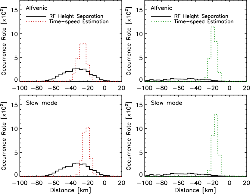
Figure 8: Comparison of RF-predicted (solid lines) and calculated (dotted lines) wave travel distances in the reference frame of the magnetic background (left) and the flux tube (right). Cases are presented for field-aligned waves propagating at the Alfvén (top) and slow-mode tube speeds (bottom). The RF-predicted vertical height separations have been converted into path length along the propagation direction.

Taking these considerations into account, the vertical height separations obtained in Sect. 3.1 are converted into path lengths along the direction of propagation. Probability distribution functions of RF-predicted path lengths from every space-time pixel are presented in Figs. 8 to 12 as solid curves, with values calculated by combining time delays, wave speeds and propagation angle to the field given as dotted (and in the case of non-vertical fast-mode waves also dashed) curves. The difference between COG values of the predicted and calculated distributions are given in Table 2 as a quantitative measure of the correspondence between the various PDFs.

A comparison between the RF-predicted and calculated path lengths of Alfvénic and slow-mode waves is presented in Fig. 8, where better correspondence is observed for the case of Alfvénic waves over that of slow modes in the MB reference frame. In the FT reference frame, however, effectively no correspondence is observed between the predicted and calculated PDFs due to the large values of field inclination. The PDF comparison for these two wave modes does not change for the differing values of originating $p$-mode propagation angle shown in Table 2 as the Alfvénic and slow modes remain directed along the magnetic field. The isotropic nature of acoustic and fast-mode waves expected in the sampled region of the atmosphere means that almost any angle of propagation could be adopted. An initial consideration of vertical propagation is provided in Fig. 9, which shows that acoustic waves yield a slightly better correspondence over fast modes, although neither can be considered successful.

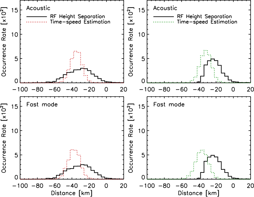
Figure 9: As for Fig. 8, but for acoustic (top) and fast-mode waves (bottom) propagating vertically.

Figure 10: As for Fig. 8, but for acoustic (top) and fast-mode waves (bottom) propagating at 40° to the vertical.

However, more appropriate values of 40°, 50°, and 60° from the vertical are presented based on the previous discussion of $p$-mode behaviour. The case of propagation at 40° to the vertical is shown in Fig. 10, where it is unclear if acoustic or fast-mode waves yield better overlap between predicted and calculated PDFs. The distributions given in Fig. 11 are arrived at when considering propagation at 50° to the vertical. In this scenario fast-mode waves appear to give better correspondence than acoustic waves in both the MB and FT reference frames, with the case of ingressing fast modes providing an improvement over that of egressing fast modes. In the final case studied, for waves propagating at 60° to the vertical, all of the PDFs in Fig. 12 show very poor correspondence when compared to the cases of 40° and 50° presented above.

Figure 11: As for Fig. 8, but for acoustic (top) and fast-mode waves (bottom) propagating at 50° to the vertical.

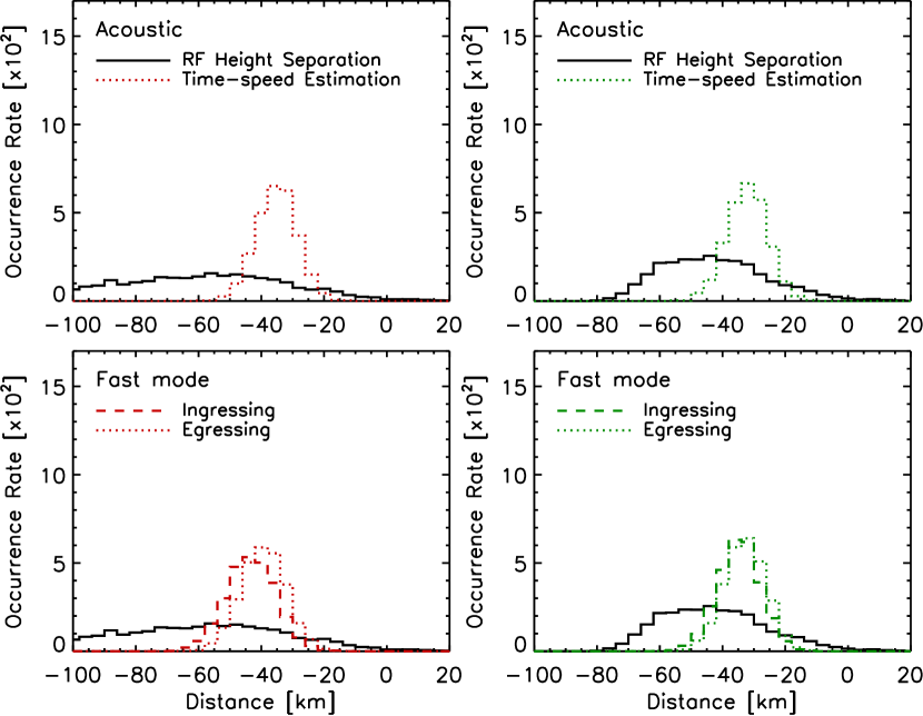
Figure 12: As for Fig. 8, but for acoustic (top) and fast-mode waves (bottom) propagating at 60° to the vertical.

4 Conclusions

Periodic LOS velocities retrieved from two atmospheric components in a sunspot penumbra have been studied to identify the form of wave mode present. The best correspondence between RF-predicted and calculated path lengths is observed for fast-mode waves propagating toward the sunspot (i.e., ingressing) at $\sim$50° to the vertical: this scenario has the smallest combination of differences between the COG separations of predicted and calculated distributions in the two reference frames (Table 2). The case for fast-mode ingression over egression is supported by the location of the sunspot being $\sim$27° from disk centre: egressing waves in the limb-side (and hence ingressing waves in the centre-side) penumbra will have a considerable component of their plasma motions directed perpendicular to our LOS and thus be difficult to observe; ingressing waves in the limb-side (and egressing waves in the centre-side) penumbra will be predominantly along our LOS. Further support is given by the horizontal wavelengths ($l\approx 870$, $\lambda\approx 5$ Mm or 7″) of the $p$-modes responsible for their excitation in the limb-side penumbra: egressing waves will have traversed two or three “skips” through the sunspot, including regions beneath either one or both of the umbrae, increasing the likelihood of their absorption or disruption; ingressing waves will be on their first “skip” into the outer region beneath the spot, remaining relatively strong and coherent. Despite the centre-side penumbra lacking strong Stokes $Q$ variations like those seen in the limb-side (because of the differing magnetic geometries with respect to the LOS), less clearly periodic velocities of $\sim$5-min period are seen there – compatible with ingressing limb-side waves being disrupted after traversing the spot. Although these data may not fully validate results from local helioseismology, in regards to wave ingression and egression, this may be possible in the future using 2-D spectropolarimetric data – e.g., using TESOS (Kentischer et al. 1998) in VIP mode – allowing direct comparison between time-distance analysis and this technique.

This is the first time that spectropolarimetric data have been used in this manner to identify a magneto-acoustic wave mode. The fact that a fast-mode wave best fits the observational data makes qualitative sense as the spectral lines used here sample a high-$\beta$ region of the deep photosphere where $p$-mode waves are expected to be modified into fast-mode waves by the presence of a magnetic field. As such, this further highlights the role that solar internal acoustic waves may play in dynamic phenomena both at and above the solar surface. It will be interesting to see if the detected form of magneto-acoustic wave changes from the case where the velocity response of a spectral line is formed below the $c_{S}=v_{A}$ (i.e., $\beta\approx 1$) surface to one where it is formed above this level. In particular, the ratio of wave amplitude, or energy content, observed both above and below the $c_{S}=v_{A}$ level may help confirm the direction of the incident $p$-mode waves (c.f., Schunker & Cally 2006).

This paper illustrates the capability of Stokes spectropolarimetry for improved wave-mode identification over imaging studies, which require an assumption about the production of intensity variations as well as inferrence of the magnetic field geometry that are usually, if at all, provided by potential field extrapolations from LOS magnetograms. The benefits of the combined determination of plasma velocities and retrieval of the full magnetic vector appear to outweigh the reduction in spatial coverage caused by using a slit-based instrument.

Finally, we note that the interpretation may depend to some extent on the model employed when carrying out the inversions. We have restricted ourselves to the simplest such two-component model. The use of more sophisticated models could lead to further refinements in the results.