A comparative study for the pair-creation contact process using series expansions

Abstract

A comparative study between two distinct perturbative series expansions for the pair-creation contact process is presented. In contrast to the ordinary contact process, whose supercritical series expansions provide accurate estimates for its critical behavior, the supercritical approach does not work properly when applied to the pair-creation process. To circumvent this problem a procedure is introduced in which one-site creation is added to the pair-creation. An alternative method is the generation of subcritical series expansions which works even for the case of the pure pair-creation process. Differently from the supercritical case, the subcritical series yields estimates that are compatible with numerical simulations.

1 Introduction

The critical properties of nonequilibrium systems have attracted attention and have seen a great development in the last years [1, 2, 3]. This may be credited to their resemblance with critical phenomena occurring in systems in thermodynamic equilibrium. In equilibrium as well as in nonequilibrium phase transitions there is a singular dependence of the steady-state properties upon the control parameters, marking a transition between distinct regimes. Other common features include long-range correlations, well-defined order parameter and singularities characterized by critical exponents that are grouped in universality classes [4].

Due to absence of a general theory for the nonequilibrium regime, these properties are analyzed in particular models, trying to form a complete picture. In particular, a class of simple models used to perform this task is constituted by lattice models with absorbing states. The presence of an absorbing state is sufficient for breaking the detailed balance condition, making these models intrinsically irreversible. In the steady-state regime, these models display a phase transition from an absorbing state to an active state, as the control parameter is varied.

A very robust universality class for these models is the directed percolation (DP) class. It describes the critical properties of any system with a phase transition between an absorbing and an active state characterized by a scalar order parameter, short-range interactions and no conservation laws [5].

Usually, the tool utilized in the study of these problems is the numerical simulation, but analytic approaches are also used as an important tool in this task leading, in some cases, to very precise results. As in other fields of physics, simulational and analytical approaches are complementary in the study of phase transitions in equilibrium and nonequilibrium systems [6]. One of these analytical approaches is the series expansion [7] that has provided the most precise estimates of the DP exponents in one-dimension [8]. Inspired by the equilibrium case, the series for nonequilibrium systems can be either supercritical or subcritical, in analogy with the high- and low-temperature expansions in equilibrium systems.

A pioneer work that uses series expansions for lattice models with absorbing states was developed by Dickman and Jensen [7], in their study of the critical properties of the contact process (CP). The contact process is an icon among the models that display a phase transition between an absorbing and active state. Initially the CP was proposed as a model for spreading of an epidemic disease [9] and has become the “Ising model” for the DP universality class. Using subcritical and supercritical series, Dickman and Jensen obtained the critical point and its associate exponents. Their results indicate that the supercritical case works better than the subcritical series.

Recently, de Oliveira [10] proposed an alternative approach for generating the subcritical expansion obtaining critical values comparable to those of the supercritical series [7]. The difference between the approaches is that in [10], the non-perturbated operator (associated with the annihilation of particles) should be diagonalized, whereas this procedure is not required for the supercritical series.

In this paper, a comparative study between subcritical and supercritical series expansion is performed for the pair-creation contact process (PCCP) [11]. Although this model does not show any surprise concerning the critical properties, since it belongs to the DP universality class as the ordinary CP, it is interesting for the comparative analysis. We will show that the original approach for the supercritical series [7] does not work properly, presenting problems in its construction. Even an alternative version of the model, that would overcome these problems, does not lead to precise results for the critical point. On the other hand, the subcritical series gives results, without any maneuver, that are comparable to those obtained by numerical simulations [12].

This paper is organized as follows. In section 2 we present the model and the operator formalism. In section 3 we show the derivation of the supercritical series, discussing its problems. In section 4, we attempt to overcome the problem by introducing a modified PCCP and deriving the supercritical series. In section 5 we present the approach for the subcritical case and results coming from the Padé analysis for both pure and modified PCCP. Finally, in section 6 the conclusions and final discussions of this work may be found.

2 Pair-creation contact process and operator formalism

We consider an interacting particle system on a one-dimensional lattice with $L$ sites. The system evolves in the time according to a Markovian process with local and irreversible rules. The configurations are described in terms of occupation variables, $\eta_{i}$, with $\eta_{i}=0,1$ according to whether the site $i$ is empty or occupied by a particle, respectively. The time evolution of the probability $P(\eta,t)$ of a given configuration $\eta\equiv(\eta_{1},\eta_{2},...,\eta_{L})$ at the time $t$ is given by the master equation,

$$\frac{d}{dt}P(\eta,t)=\sum_{i}^{L}\{w_{i}(\eta^{i})P(\eta^{i},t)-w_{i}(\eta)P(\eta,t)\},$$ (1)

where $\eta^{i}\equiv(\eta_{1},\eta_{2},...,1-\eta_{i},...,\eta_{L})$. The transition rate $w_{i}(\eta)$ for the PCCP is given by

$$w_{i}(\eta)=\frac{1}{2}(1-\eta_{i})(\eta_{i-2}\eta_{i-1}+\eta_{i+1}\eta_{i+2})+\alpha\eta_{i}.$$ (2)

If an empty site has two occupied neighbor sites, then this site becomes occupied with a transition rate equals to $n/2$, where $n$ is the number of the pairs of the first neighbors occupied. If the site is occupied, then it is becomes empty with a rate $\alpha$, independently of its neighborhood.

When the lattice is entirely empty, the system is trapped in an absorbing state. However, for small values of the rate $\alpha$, an active state can be achieved in the stationary state. In this way, a continuous phase transition occurs in this model with the critical point localized, according to simulational results [12], in $\alpha_{c}=0.1341(6)$.

To develop this operator formalism, we represent the microscopic configurations of the lattice by the direct product of vectors

$$|\eta\rangle=\bigotimes_{i}|\eta_{i}\rangle.$$ (3)

The algebra is defined by the creation and annihilation operators for the site $i$

$$A_{i}^{\dagger}|\eta_{i}\rangle = (1-\eta_{i})|\eta_{i}+1\rangle,$$

$$A_{i}|\eta_{i}\rangle = \eta_{i}|\eta_{i}-1\rangle.$$ (4)

In this formalism, the state of the system at time $t$ may be represent as

$$|\psi(t)\rangle=\sum_{\{\eta\}}P(\eta,t)|\eta\rangle.$$ (5)

If we define the projection onto all possible states as

$$\langle\mbox{ }|\equiv\sum_{\{\eta\}}\langle\eta|,$$ (6)

the normalization of the state may be expressed as $\langle\mbox{ }|\psi\rangle=1$.

The master equation (1) can be shown to be equivalent to the following time evolution equation

$$\frac{d}{dt}|\psi(t)\rangle=S|\psi(t)\rangle,$$ (7)

where $S$ is the evolution operator, given by

$$S=S_{p}+\alpha S_{a},$$ (8)

where

$$S_{p}=\frac{1}{2}\sum_{i}\{(A_{i}^{\dagger}-A_{i}A_{i}^{\dagger})(A_{i-2}^{\dagger}A_{i-2}A_{i-1}^{\dagger}A_{i-1}+A_{i+1}^{\dagger}A_{i+1}A_{i+2}^{\dagger}A_{i+2})\}$$ (9)

is the pair-creation operator and

$$S_{a}=\sum_{i}(A_{i}-A_{i}^{\dagger}A_{i})$$ (10)

is the annihilation operator.

3 Supercritical series expansion

By rescaling the time, it is possible to rewrite the evolution operator as

$$S=V+\mu W,$$ (11)

where $W=S_{a}$, $V=2S_{p}$ and $\mu=2\alpha$. Since the operator $W$ is associated to annihilation process and the creation of particle is present in the operator $V$, for small values of the parameter $\mu$ the creation process is favored, so that the composition above is convenient for a supercritical series. The action of each operator, in a general configuration $(\mathcal{C})$, is explicitly shown by the expressions

$$W(\mathcal{C})=\sum_{i=1}^{r}(\mathcal{C}_{i}^{\prime})-r(\mathcal{C}),$$ (12)

and

$$V(\mathcal{C})=\sum_{i=1}^{p_{1}}(\mathcal{C}_{i}^{\prime\prime})+2\sum_{i=1}^{p_{2}}(\mathcal{C}_{i}^{\prime\prime})-(p_{1}+2p_{2})(\mathcal{C}),$$ (13)

where $r$ is the occupied sites number, $(\mathcal{C}_{i}^{\prime})$ is obtained replacing a particle at the site $i$ by a hole, while $p_{1}$ and $p_{2}$ are the number of the empty sites with one and two occupied pair of neighbors, respectively. Finally, $(\mathcal{C}_{i}^{\prime\prime})$ is the configuration obtained replacing the hole at the site $i$ by a particle.

Since we are interested in the steady-states properties, it is convenient to take the Laplace transform of the state vector, given by

$$|\tilde{\psi}(s)\rangle=\int_{0}^{\infty}e^{-St}|\psi(t)\rangle.$$ (14)

Inserting the formal solution given by the equation (7), we find

$$|\tilde{\psi}(s)\rangle=(s-S)^{-1}|\psi(0)\rangle.$$ (15)

The stationary state $|\psi(\infty)\rangle\equiv\lim_{t\to\infty}|\psi(t)\rangle$ may then be found noticing that

$$|\psi(\infty)\rangle=\lim_{s\to 0}s|\tilde{\psi}(s)\rangle,$$ (16)

which is obtained integrating equation (14) by parts. Assuming that $|\tilde{\psi}(s)\rangle$ may be expanded in powers of $\mu$ and using equation (15), we have that

$$|\tilde{\psi}(s)\rangle=|\tilde{\psi}_{0}\rangle+\mu|\tilde{\psi}_{1}\rangle+\mu^{2}|\tilde{\psi}_{2}\rangle+\cdots=(s-V-\mu W)^{-1}|\psi(0)\rangle.$$ (17)

Expanding the operator $(s-V-\mu W)^{-1}$ in powers of $\mu$,

$$(s-V-\mu W)^{-1}=(s-V)^{-1}\left[1+\mu(s-V)^{-1}W+\mu^{2}(s-V)^{-2}W^{2}+\cdots\right],$$ (18)

and comparing each order in $\mu$, we arrive at the expressions:

$$|\tilde{\psi}_{0}\rangle=(s-V)^{-1}|\psi(0)\rangle,$$ (19)

and

$$|\tilde{\psi}_{n}\rangle=(s-V)^{-1}W|\tilde{\psi}_{n-1}\rangle,$$ (20)

for $n\neq 0$.

The action of the operator $(s-V)^{-1}$ on an arbitrary configuration $({\mathcal{C}})$ may be found noticing that

$$(s-V)^{-1}({\mathcal{C}})=s^{-1}\left\{({\mathcal{C}})+(s-V)^{-1}V({\mathcal{C}})\right\},$$ (21)

and using the expression (13) for the action of the operator $V$, we get

$$(s-V)^{-1}({\mathcal{C}})=s_{q}\left\{({\mathcal{C}})+(s-V)^{-1}\left[\sum_{i=1}^{p_{1}}({\mathcal{C}}^{\prime\prime}_{i})+2\sum_{j=1}^{p_{2}}({\mathcal{C}}^{\prime\prime}_{j})\right]\right\},$$ (22)

where $s_{q}\equiv 1/(s+q)$ and $q=p_{1}+2p_{2}$.

The main obstacle to generate the standard supercritical series for this model is due the action of the operator $(s-V)^{-1}$ over a configuration $(\mathcal{P})$ without pairs of particles, whose result is given by

$$(s-V)^{-1}(\mathcal{P})=\frac{1}{s}(\mathcal{P}).$$ (23)

The successive action of $(s-V)^{-1}$ over the configuration $(\mathcal{P})$ or their offsprings will result in new configurations whose associated coefficient will be proportional to $s^{-n}$ ($n>1$) and thus, it diverges in the stationary state. To overcome this difficulty, we present in the next section an alternative version of PCCP model that avoid this divergence and, in principle, enables us to find asymptotic results for the critical properties of the PCCP model.

4 Pair-creation contact process modified by a single creation transition

The modification consists of adding to the transition rate (2) a term of creation by single particles similar to the ordinary contact process [1], so that the transition rate is given by

$$w_{i}(\eta)=\frac{1}{2}(1-\eta_{i})\{\eta_{i-2}\eta_{i-1}+\eta_{i+1}\eta_{i+2}+\gamma(\eta_{i-1}+\eta_{i+1})\}+\alpha\eta_{i}.$$ (24)

The operator $V$ in equation (11) now reads $V=2(S_{p}+\gamma S_{s})$, where the single creation operator $S_{s}$ is given by

$$S_{s}=\frac{1}{2}\sum_{i}\{(A_{i}^{\dagger}-A_{i}A_{i}^{\dagger})(A_{i-1}^{\dagger}A_{i-1}+A_{i+1}^{\dagger}A_{i+1})\}.$$ (25)

In the limit of $\gamma\rightarrow 0$, we recover the pure PCCP model.

The operator $W$ acts over $(\mathcal{C})$ according to equation (12), whereas the action of the operator $(s-V)^{-1}$ is given by

$$(s-V)^{-1}(\mathcal{C}) = s_{p,\gamma}\left\{(\mathcal{C})+(s-V)^{-1}\left[\sum_{i=1}^{p1}(\mathcal{C}_{i}^{\prime\prime})+2\sum_{i=1}^{p_{2}}(\mathcal{C}_{i}^{\prime\prime})\right]\right\}+$$ (26)

$$+ s_{p,\gamma}\gamma\left\{(s-V)^{-1}\left[\sum_{i=1}^{r_{1}}(\mathcal{C}_{i}^{\prime\prime})+2\sum_{i=1}^{r_{2}}(\mathcal{C}_{i}^{\prime\prime})\right]\right\},$$

where $s_{p,\gamma}=(s+[p_{1}+p_{2}]+\gamma[r_{1}+r_{2}])^{-1}$, $p_{1}$ and $p_{2}$ (are the number of empty sites with one and two pairs of occupied neighbors, respectively and $r_{1}$ and $r_{2}$ are the number of empty sites with one and two occupied neighbors, respectively. The expression $(\mathcal{C}_{i}^{\prime\prime})$ corresponds to the configuration obtained by replacing a hole at site $i$ by a particle. Differently from the pure PCCP, the modified PCCP does not have divergences when one takes the limit $s\rightarrow 0$. Thus, for configurations $(\mathcal{P})$, we have that

$$(s-V)^{-1}(\mathcal{P})=\frac{1}{s+\gamma b}\left\{(\mathcal{P})+\sum_{j}(\mathcal{P}^{j})\right\},$$ (27)

where $b$ is an integer number and $(\mathcal{P}^{j})$ is a configuration originated from $(\mathcal{P})$ by a simple creation process. The particular case of the vacuum $(0)$ for which $(s-V)^{-1}(0)=1/s(0)$ does not diverge in the stationary state limit.

In the supercritical expansion the operator $(s-V)^{-1}$ acting over any configuration (except the vacuum) generating an infinite set of configurations, so it is impossible to evaluate $|{\tilde{\psi}(s)}\rangle$ in a closed form. We can evaluate, however, the ultimate survival probability $P_{\infty}$, which corresponds to the coefficient of the vacuum. We define the series coefficients as

$$P_{\infty}=1-\sum_{i}a_{i}(\gamma)\alpha^{i}.$$ (28)

Using a proper computational algorithm, we can calculate the coefficients up to order 23, with values of $\gamma$ shown in figure 1. The limiting factor for this calculation is actually the memory required. We attempt to obtain the critical properties of the PCCP model by performing the numerical extrapolation $\gamma\to 0$, since this approach does not work in the case $\gamma=0$.

To analyze the series, we use the d-log Padé approximants approach. These approximants are defined as ratios of two polynomials

$$\frac{P_{L}(\alpha)}{Q_{M}(\alpha)}=\frac{\sum_{i=0}^{L}p_{i}\alpha^{i}}{1+\sum_{j=1}^{M}q_{j}\alpha^{j}}=f(\alpha).$$ (29)

In our case the function $f(\alpha)$ represents the series for $\frac{d}{d\alpha}\ln P_{\infty}(\alpha)$, for a fixed value for the parameter $\gamma$. Therefore, we are able to obtain approximants satisfying the condition $L+M\leq 22$. One verifies that diagonal ($L=M$) and near-diagonal approximants usually exhibit better convergence properties, so that we will restrict our calculations to the set of approximants such that $L=M+\theta$, with $\theta=0,\pm 1$.

In the neighborhood of the critical point the ultimate survival probability behaves as $P_{\infty}\sim(\alpha_{c}-\alpha)^{\beta}$. The critical point $\alpha_{c}$ is determined by the pole of the approximant $F_{LM}(\alpha)$ and the exponent $\beta$ by the residue associated with this pole.

In figure 1 the estimates for critical points $\alpha_{c}$ are depicted for different values of the parameter $\gamma$. Using a linear extrapolation of these data, we obtain the estimation for the asymptotic limit $\gamma\rightarrow 0$ as $\alpha_{c}=0.1398(7)$, in disagreement with the simulational result $\alpha_{c}=0.1341(6)$ [12]. We remark that decreasing the parameter $\gamma$, the dispersion of the approximants increases and the precision of the result becomes smaller.

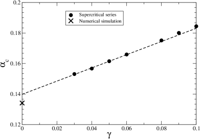
Figure 1: Critical line in the plane $\alpha$ versus $\gamma$ for the modified PCCP model by supercritical series (circles). The dashed line is a linear extrapolation toward $\gamma=0$. For comparison, we plotted the numerical simulation result (cross).

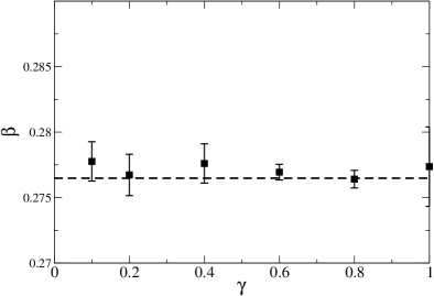
Figure 2: Exponent $\beta$ for the modified PCCP model as a function of $\gamma$.

The exponent $\beta$, as shown in figure 2, is in accordance with the DP universality class value for any value of the parameter $\gamma$, as expected.

However, the uncertainties on the location of the critical point put in doubt the accuracy of the supercritical series around $\gamma\approx 0$. In fact, what happens is that the coefficients of the configurations $(\mathcal{P})$ in the steady-state behaves as

$$(s-V)^{-1}(\mathcal{P})\sim\frac{1}{\gamma b}(\mathcal{P}),$$ (30)

diverging as $\gamma\to 0$. This behavior causes a ill-conditioned series for $\gamma\approx 0$, becoming impossible a more accurate result for the critical point in this limit.

5 Subcritical series expansion

To develop subcritical series expansion, we rewrite the evolution operator as

$$S=W+\lambda(S_{p}+\gamma S_{s}),$$ (31)

where $\lambda=\alpha^{-1}$. Since the operator $W$ is associated to annihilation process and, for small values of the parameter $\lambda$, this annihilation process is favored, this expansion describes indeed the subcritical regime. Differently from the supercritical case, the series here are generated directly, without the necessity of taking the Laplace transform.

The operator $W$, associated to annihilation particles process, is expressed as $W=\sum_{i}W_{i}$, with $W_{i}=A_{i}-A_{i}^{\dagger}A_{i}$. Each term $W_{i}$ has the following set of right and left eigenvectors

$$|0\rangle\equiv|\circ\rangle,\hskip 28.45274pt\langle 0|\equiv\langle\circ|+\langle\bullet|,$$ (32)

with eigenvalue $\Lambda_{0}=0$ and

$$|1\rangle\equiv-|\circ\rangle+|\bullet\rangle,\hskip 28.45274pt\langle 1|\equiv\langle\bullet|,$$ (33)

with eigenvalue $\Lambda_{1}=-1$.

To find the steady state vector $|\psi\rangle$, that satisfies the steady condition $S|\psi\rangle=0$, we assume that

$$|\psi\rangle=|\psi_{0}\rangle+\sum_{\ell=1}^{\infty}\lambda^{\ell}|\psi_{\ell}\rangle,$$ (34)

where $|\psi_{0}\rangle$ is the steady solution of the non-interacting term $W$ satisfying the stationary condition

$$W|\psi_{0}\rangle=0.$$ (35)

The vectors $|\psi_{\ell}\rangle$ can be generated recursively from the initial state $|\psi_{0}\rangle$. Following Dickman [13], we get the recursion relation

$$|\psi_{\ell}\rangle=-R(S_{p}+\gamma S_{s})|\psi_{\ell-1}\rangle.$$ (36)

The operator $R$ is the inverse of $W$ in the subspace of vectors with eigenvalues and is given by

$$R=\sum_{n(\neq 0)}|\phi_{n}\rangle\frac{1}{\Lambda_{n}}\langle\phi_{n}|,$$ (37)

where $|\phi_{n}\rangle$ and $\langle\phi_{n}|$ are right and left eigenvectors of $W$, respectively, with nonzero eigenvalue $\Lambda_{n}$. Since the creation of particles is catalytic, if we start from steady state of the noninteracting term, that corresponds to the vacuum state, we will obtain a trivial steady vector. To overcome this problem, it is necessary to introduce a modification on the rules of the model. The necessity of changing the initial state in systems with absorbing states in order to get nontrivial steady states have been considered previously by Jensen and Dickman [7, 14] and more recently by de Oliveira [10].

The modification we have performed [10] consists in introducing a spontaneous creation of particles. For the case $\gamma=0$ (pure PCCP) the creation occurs in two adjacent sites, chosen to be $i=0$ and $i=1$. This modification leads to the following expression to the operator $W$

$$W=\sum_{i}W_{i}+q(U_{0}+U_{1}-W_{0}-W_{1}),$$ (38)

where $q$ is supposed to be a small parameter and $U_{i}=A_{i}^{\dagger}-A_{i}A_{i}^{\dagger}$. The steady state $|\psi_{0}\rangle$ of $W$ is not the vacuum state anymore. Now, it is given by

$$|\psi_{0}\rangle=|.0.\rangle+2q|.10.\rangle+q^{2}|.11.\rangle,$$ (39)

where all sites before and after the symbol “.” are empty.

Two remarks are in order. First, only the last term in $|\psi_{0}\rangle$ will give nonzero contributions to the expansion so that $|\psi_{\ell}\rangle$, $\ell\geq 1$, will be of the order $q^{2}$. Second, Although the change in $W$ will cause a change in $R$, only the terms of zero order in the expansion in $q$, given by the right-hand side of equation (37), will be necessary since the corrections in $R$ will contribute to terms of order larger than $q^{2}$. For instance, the two first vectors, $|\psi_{1}\rangle$ and $|\psi_{2}\rangle$, for the pure PCCP are given by

$$|\psi_{1}\rangle=q^{2}\{2|.1.\rangle+|.11.\rangle+|.101.\rangle+\frac{2}{3}|.111.\rangle\},$$ (40)

and

$$|\psi_{2}\rangle=q^{2}\{\frac{2}{3}|.1.\rangle+\frac{1}{3}|.11.\rangle+\frac{1}{3}|.101.\rangle+\frac{2}{9}|.111.\rangle+$$

$$+\frac{2}{3}|.1001.\rangle+\frac{4}{9}|.1101.\rangle+\frac{4}{9}|.1011.\rangle+\frac{1}{3}|.1111.\rangle\},$$ (41)

where the translational invariance of the system is assumed.

For $\gamma\neq 0$, it suffices to consider the spontaneous creation in just one site. This modifications leads to the following expression

$$W=\sum_{i}W_{i}+q(U_{0}-W_{0}),$$ (42)

instead of equation (38).

From the series expansion of the state vector $|\psi\rangle$, it is possible to determine several quantities. In this paper, we will be concerned only with the series expansion for the total number of particles $N$, given by

$$N=\langle.0.|\sum_{i}n_{i}|\psi\rangle.$$ (43)

One can show that the coefficient of $\lambda^{\ell}$ in the expansion for $N$ is simply the coefficient of $|.1.\rangle$ in $|\psi_{\ell}\rangle$. This allows us to get a longer series for the number of particles. For both modified and pure PCCP, we have obtained a series with 38 terms.

The critical behavior of $N$ obeys the following relation [10]

$$N\sim(\alpha_{c}-\alpha)^{-\nu_{\,||}(1+\eta)},$$ (44)

where $\nu_{\,||}$ and $\eta$ are the exponents related to the time correlation length and to the growth of the number of particles, respectively. Through an analysis of the d-log Padé approximants, like that performed for supercritical series expansion, we are able to calculate the critical point and its associated exponent. Using the series for the number of particles $N$ the values obtained were $\alpha_{c}=0.1310(14)$ and $\nu_{\parallel}(1+\eta)=2.68(15)$. These values do not agree with the best estimates, $\alpha_{c}=0.1341(6)$ [12] and $\nu_{\parallel}(1+\eta)=2.2777305$ [8]. Another estimate is obtained by performing a non-homogeneous d-log Padé approximant [15]. Using this approach we obtained the value $\alpha_{c}=0.1337(17)$, closer to the value obtained by numerical simulations [12].

More reliable estimates are obtained when we determine the Padé approximants for the series $(\alpha_{c}-\alpha)(d/d\alpha)$ ${\rm ln}N=\theta$ [7, 16], called biased Padé approximants. Considering a given Padé approximant $[L/M]$ and a trial value of $\tilde{\alpha}_{c}$, we develop the series above obtaining $\theta(\tilde{\alpha}_{c})$. We can build curves for different Padé approximants by repeating this procedure for several trials $\tilde{\alpha}_{c}$ and we expect that they intercept at the critical point ($\alpha_{c}$, $\theta(\alpha_{c})$).

Figure 3: Biased estimates of $\theta=\nu_{\,||}(1+\eta)$ as a function of $\tilde{\alpha_{c}}$ derived from Padé approximants to the series $(\tilde{\alpha_{c}}-\alpha)(d/d\alpha)$ $\ln N=\theta$ evaluated at $\tilde{\alpha}_{c}$ for the PCCP. The approximants shown are [17/18], [18/17], [18/18], [18/19], and [19/18].

From the figure 3 we see a very narrow intersection of the Padé approximants, revealing the utility of this approach. However, as pointed out by Guttmann [17], it is difficult to estimate uncertainties in series calculations. Thus, in order to give a more realistic estimate of the quantities measured here and their associated uncertainties, we have estimated them by taking into account the first and last crossings among various Padé approximants. The estimate of $\alpha_{c}$ for the PCCP, $\alpha_{c}=0.13396(1)$, in excellent agreement with the corresponding value obtained from recent numerical simulations [12]. Finally, the exponent obtained is $\nu_{\parallel}(1+\eta)=2.274(3)$, in agreement with the best estimation of $\nu_{\parallel}(1+\eta)$ for the DP universality class [8].

To stress the difference between subcritical and supercritical approaches, we have also developed subcritical series expansion for the modified PCCP model for some values of $\gamma$, as shown in figure 4. In the limit $\gamma\rightarrow 0$, the subcritical approach gives $\alpha_{c}=0.1340(1)$, which is in good agreement with the estimate $\alpha_{c}=0.13396(1)$ for $\gamma=0$ and $\alpha_{c}=0.1341(6)$ obtained from numerical simulations [12]. On the other hand, the extrapolation for $\gamma\rightarrow 0$ in the supercritical case does not lead to the correct value, as can be seen in figure 1.

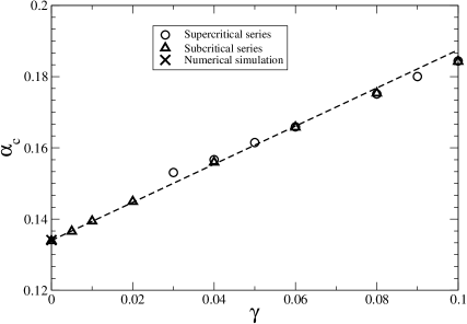
Figure 4: Comparative results for the modified PCCP model using supercritical (circles), subcritical (triangles) series and numerical simulations (cross).

6 Conclusions

In this work, we have considered the pair-creation contact process by carrying out a comparative study between subcritical and supercritical expansions. Differently from the contact process, the supercritical expansion in its canonical formulation [7] is intrinsically ill-conditioned for the PCCP. In fact, divergences in coefficients of the supercritical series occur for any model with creation by cluster of particles. As an attempt to circumvent the divergences, we introduced and analyzed a modified version of the PCCP. However this procedure does not lead to the correct result when one recovers the original model. It would be interesting to search an alternative procedure to develop supercritical series for such models. We have shown here that subcritical series expansion provides results comparable with recent numerical simulations [12].

A natural extension of this work is the use of subcritical series to study models with creation by clusters (pairs and triplets) and diffusion of particles [11, 12]. Results from numerical simulations [12, 18] suggest that these models display a tricritical point. Thus this approach, associated with an analysis by means of partial differential approximants in two-variables, could be used to determine the existence of a tricritical point. In fact, such an approach has already been shown to be useful for the location of a multicritical point in a generalized contact process [16].

References

References

- [1] J. Marro and R. Dickman, Nonequilibrium Phase Transitions in Lattice Models (Cambridge University Press, Cambridge, 1999)
- [2] Nonequilibrium Statistical Mechanics in One Dimension edited by V. Privman, (Cambridge University Press, Cambridge, 1997)
- [3] H. Hinrichsen, Phys. A 1, 369 (2006).
- [4] G. Odor, Rev. Mod. Phys. 76, 663 (2004).
- [5] H. K. Janssen, Z. Phys. B, 42, 151 (1981); P. Grassberger, Z. Phys. B, 47, 365 (1982).
- [6] H. Hinrichsen, Adv. in Phys. 49, 815 (2000).
- [7] I. Jensen and R. Dickman, J. Stat. Phys. 71, 89 (1993).
- [8] I. Jensen, J. Phys. A 32, 5233 (1999).
- [9] T. E. Harris, Ann. Probab. 2, 969 (1974).
- [10] M. J. de Oliveira, J. Phys. A 39, 11131 (2006).
- [11] R. Dickman and T. Tomé, Phys. Rev. A 44, 4833 (1991).
- [12] C. E. Fiore and M. J. de Oliveira, Phys. Rev. E, 70, 046131 (2004).
- [13] R. Dickman, J. Stat. Phys. 55,997 (1989).
- [14] I. Jensen and R. Dickman, Physica A 203, 175 (1994).
- [15] F. D. A. A. Reis and R. Rieira, Phys. Rev. E 49, 2579 (1994).
- [16] W. G. Dantas and J. F. Stilck, J. Phys. A 38, 5841 (2005).
- [17] C. Domb and J. L. Lebowitz (eds) Phase Transitions and Critical Phenomena vol 13, (New York, Academic Press, 1989).
- [18] G. Cardozo and J. F. Fontanari, Eur. Phys. Journal B, 51 555 (2006).