The $\beta$-Model Problem: The Incompatibility of X-ray and Sunyaev-Zeldovich Effect Model Fitting for Galaxy Clusters

Abstract

We have analyzed a large sample of numerically simulated clusters to demonstrate the adverse effects resulting from use of X-ray fitted $\beta$-model parameters with Sunyaev-Zeldovich effect (SZE) data. There is a fundamental incompatibility between $\beta$ fits to X-ray surface brightness profiles and those done with SZE profiles. Since observational SZE radial profiles are in short supply, the X-ray parameters are often used in SZE analysis. We show that this leads to biased estimates of the integrated Compton y-parameter inside $r_{500}$ calculated from clusters. We suggest a simple correction of the method, using a non-isothermal $\beta$-model modified by a universal temperature profile, which brings these calculated quantities into closer agreement with the true values.

1. Introduction

The hot gas in clusters of galaxies is responsible for inverse Compton scattering cosmic microwave background (CMB) photons as they travel through the intracluster medium (ICM). This results in a spectral distortion of the CMB at the location of clusters on the sky, referred to as the Sunyaev & Zeldovich (1972) effect (SZE). This distortion is characterized by a low frequency ($<$218 GHz) decrement, and higher frequency ($>$218 GHz) increment in the CMB intensity (Carlstrom et al., 2002). The X-ray emission in clusters consists of thermal bremsstrahlung and line emission from the same highly ionized plasma that scatters the CMB.

High resolution X-ray or SZE observations of clusters coupled with assumptions about the gas distribution lead to estimates of the gas mass in the cluster dark matter potential well. The electron number density is often assumed to fit a $\beta$ model (Cavaliere & Fusco-Femiano, 1978),

$$n_{e}(r)=n_{e0}\left(1+\left(\frac{r}{r_{c}}\right)^{2}\right)^{-3\beta/2}.$$ (1)

In the above relation, $n_{e0}$ is the central density normalization and $r_{c}$ indicates the fitted parameter referred to as the core radius. Fitting an observed X-ray or SZE profile to these projected $\beta$ model X-ray surface brightness and SZE $y$ parameter distributions results in a description of the density distribution, which can be integrated to obtain the gas mass. The difference in dependence on gas density and temperature of X-ray emissivity and the SZE $y$ parameter makes the combination of these two methods of observation potentially very powerful. Because of this difference, the observability of clusters via each method is affected differently by the impact of physics in cluster cores including radiative cooling and feedback mechanisms, as well as the transient boosting of surface brightness and spectral temperature generated during merging events (Roettiger et al., 1996; Motl & Burns, 2005). These two methods not only select a different sample of clusters, but combined SZE/X-ray observations of individual clusters allow one to extract the density and temperature of the gas without relying on X-ray spectral temperatures.

1.1. Isothermal Beta Models

Under the assumption that the gas in clusters is isothermal, one can fit an isothermal $\beta$-model to the data in order to deduce the density profile. To generate the projected X-ray surface brightness profile, we integrate the $\beta$-model density distribution

$$S_{X}=\frac{1}{4\pi(1+z)^{4}}\int n_{e}(r)n_{H}(r)\Lambda(T)dl,$$ (2)

where in the bremsstrahlung limit, $\Lambda(T)\propto T^{1/2}$, and in a fixed X-ray band is more weakly dependent on temperature (Mohr et al., 1999). This integration results in

$$S_{X}(b)=S_{X0}\left(1+\left(\frac{b}{r_{c}}\right)^{2}\right)^{\frac{1}{2}-3\beta},$$ (3)

where $S_{X0}$ is the fitted central X-ray surface brightness of the model, and $b$ indicates the projected radius. Similarly for the SZE, a $\beta$-model density profile can be integrated

$$y=\int\sigma_{T}n_{e}(r)\frac{k_{b}T}{m_{e}c^{2}}dl,$$ (4)

which results in a projected radial distribution of the Compton $y$ parameter

$$y(b)=y_{0}\left(1+\left(\frac{b}{r_{c}}\right)^{2}\right)^{\frac{1}{2}-\frac{3\beta}{2}}.$$ (5)

For very hot clusters (T $>$ 10 keV), relativistic corrections must be included to the SZE integral (Itoh & Nozawa, 2004). While these fits result in a description of the cluster density profile, we must be aware that that description is only approximate, since it has been shown both in simulations and observations (Loken et al., 2002; Vikhlinin et al., 2005) that many clusters show a radial dependence of temperature. That means that when using isothermal models (the above equations) to fit the data, we should expect error to be introduced in the derived quantities.

1.2. SZE/X-ray Derived Quantities

Recent studies have used the values of the $\beta$-model parameters determined from the X-ray surface brightness profiles combined with SZE cluster observations to determine the value of the Hubble constant ($H_{0}$) (Reese et al., 2002; Bonamente et al., 2006) and the cluster gas fraction (Joy et al., 2001; LaRoque et al., 2006). While joint fits of X-ray and SZE interferometric data are used to determine the $\beta$-model parameters in these studies, the X-ray data drives the fit, since the SZE data currently lacks the resolution (and interferometric U-V plane coverage) to constrain the parameters well (LaRoque et al., 2006).

An additional calculation can be performed using combined SZE/X-ray data from clusters. It is expected both from analytic arguments and numerical simulations that the integrated SZE signal, as a measure of the total ICM pressure in clusters, should be an excellent proxy for cluster total mass (da Silva et al., 2000; Motl et al., 2005; Nagai, 2006; Kravtsov et al., 2006). This presupposes that one can determine accurately the value of the integrated SZE signal to some mass-scaled cluster radius, as well as perform an accurate calibration of this relationship observationally. In Motl et al. (2005), we showed that the value of $Y_{500}$, the integrated Compton $y$ parameter inside a radius where $\delta\rho/\rho$ = 500 (with respect to the critical density) accurately measures the cluster total mass inside that same radius. In order to accurately calibrate this relationship, one must measure the $Y$-$M$ relationship to high precision at low redshift, where clusters have combined SZE/X-ray observations to use. Then the measured relation, scaled for redshift, can be used to determine masses of SZE-selected clusters, which should be indentifiable to high redshifts, in order to constrain cosmology.

Since SZE radial profiles are of relatively poor quality so far, a direct determination of the compatibility of the X-ray $\beta$-model parameters with the SZE profiles in clusters can not currently be done observationally. Here we compare the values of $\beta$-model parameters for a large number of simulated clusters when fitting the X-ray surface brightness profile, the SZE radial Compton $y$ profile, and jointly fitting both X-ray and SZE profiles to a common $\beta$-model. We show that the use of X-ray parameter values leads to biased estimates of $Y_{500}$, as well as the integrated gas mass $M_{500,gas}$.

We discuss our numerical simulations in Section 2, results of the analysis in Section 3, the consequences of the use of X-ray $\beta$-model parameters for estimating the $Y_{500}$-$M_{500}$ relationship for clusters in Section 4, and discussion and conclusions in Section 5.

2. Numerical Simulations

Our simulations use the hybrid Eulerian adaptive mesh refinement hydro/N-body code Enzo (O’Shea et al. (2005); http://cosmos.ucsd.edu/enzo) to evolve both the dark matter and baryonic fluid in the clusters, utilizing the piecewise parabolic method (PPM) for the hydrodynamics. With up to seven levels of refinement in high density regions, we attain spatial resolution up to $\sim\;16\;h^{-1}$ kpc in the clusters. We assume a concordance $\Lambda$CDM cosmological model with the following parameters: $\Omega_{\mathrm{b}}=0.026$, $\Omega_{\mathrm{m}}=0.3$, $\Omega_{\Lambda}=0.7$, $\mathrm{h}=0.7$, and $\sigma_{8}=0.9$. Refinement of high density regions is performed as described in Motl et al. (2004).

We have constructed a catalog of AMR refined clusters identified in the simulation volume as described in Loken et al. (2002). The catalog of clusters used in this study includes the effects of radiative cooling, models the loss of low entropy gas to stars, adds a moderate amount of supernova feedback due to Type II supernovae in the zones where stars form, and is identified as the SFF (Star Formation with Feedback) catalog in Hallman et al. (2006). The catalog includes clusters with total mass (baryons + dark matter) greater than $10^{14}M_{\odot}$ out to z=2 in the simulation. This catalog includes roughly 100 such clusters at z=0, and has 20 redshift intervals of output, corresponding to a total of roughly 1500 clusters in all redshift bins combined.

For parts of the analysis, we have cleaned the cluster sample as described in Hallman et al. (2006), removing cool core clusters and obviously disturbed clusters. This is done primarily to more closely mimic observational studies of cluster properties. We examine by eye all cluster projections and remove any with obvious double peaks in the X-ray or SZE surface brightness images, have disturbed morphology within R = $1h^{-1}$ Mpc, exhibit edges consistent with shocked gas, or those that have cool cores. The cool core clusters are identified as those with a projected emission-weighted temperature profile which declines at small radius, or those with strongly peaked X-ray emission. The cool core clusters are eliminated because as we have shown in Hallman et al. (2006), they lead to strong biases and increased scatter in estimates of cluster physical properties when standard observational methods are used. We show in our previous work that eliminating obviously disturbed clusters has a minor, but measurable effect on observationally derived quantities. Indeed the simple assumptions that are typically made in the observational derivation (e.g., spherical symmetry, hydrostatic equilibrium) clearly do not apply to such clusters. We also use two orthogonal projected images for each cluster. The final cleaned sample contains 493 cluster projected images from a series of evolutionary epochs from z=0 to z=2.

3. Results

3.1. Isothermal $\beta$-model Fits

Figure 1.— Upper panels: Left panel shows comparison of fitted $\beta$ values for clusters in our numerical sample at z=0 out to $r_{2500}$ using the X-ray and SZE images. Right panel shows comparison of fitted value of $r_{c}$ for same clusters. Middle panels: Same as above, except values are for profiles fitted out to $r{500}$. Lower panels: Same as above, but for profiles fitted out to $r_{200}$.

We have generated images of our simulated cluster catalog by projecting the physical quantities on the grid to get the value of the SZE Compton $y$ parameter and the X-ray surface brightness. For the X-ray, we have used a simple bremsstrahlung emissivity. It is a simpler calculation than using a model X-ray emissivity, and we will show later that the values of the $\beta$-model parameters are nearly identical irrespective of which emissivity calculation we use.

From these images, we have created radial profiles in annular bins, which we subsequently fit to $\beta$-model profiles. Each cluster, for both the SZE and X-ray profile, has a set of $\beta$-model parameters that describe it, though there is some degeneracy in the parameters in each case. The three $\beta$-model parameters, namely the normalization ($S_{X0}$ or $y_{0}$), the value of the core radius ($r_{core}$), and the power law index $\beta$ are left as free parameters in the fit. We have fit to each of three limiting outer radii in both the SZE and X-ray case, $r_{2500}$, $r_{500}$, and $r_{200}$. In each case, the subscript indicates the average overdensity with respect to critical inside that radius. This radius is calculated from the simulation data using the overdensity of the dark matter. We have used the full sample for this part of the analysis, but have excluded the cool core region (typically $\approx$100kpc) of the profiles from the fitting procedure.

We have found that there are significant differences in the values of the fitted model parameters depending on whether the X-ray or SZE profiles are used. Figure 1 shows the comparison of the values of $\beta$ and $r_{core}$ plotted against one another for individual z=0 clusters in our catalog for the three limiting outer radii used. It is clear that there is a large amount of scatter in the relationship for the $\beta$ values, and also at $r_{500}$ and $r_{200}$, a definite discrepancy. Fitting SZE profiles results in a consistently higher value of $\beta$ than does fitting X-ray profiles. While there is scatter in the compared values of $r_{core}$, there is general agreement within the errors. However, since there is a degeneracy between $r_{core}$ and $\beta$ in the fitting, some scatter is expected. Since the values of $\beta$ and $r_{core}$ are used directly in the equation for the density profile, inconsistent values for these parameters lead to different deduced density profiles, and discrepant values for the cluster gas mass.

Figure 2.— Upper: Ratio of SZE $\beta$ fitted to radial profiles from projections of full SFF simulated sample of clusters to $\beta$ fitted to X-ray radial profiles for the same clusters. Median values and 1$\sigma$ error bars for the ratio $\beta_{SZE}/\beta_{X-ray}$ in z=0 clusters fitted to each of three radii $r_{2500}$, $r_{500}$, and $r_{200}$ using the isothermal $\beta$-model. Lower: Median values and 1$\sigma$ error bars for the ratio $r_{core,SZE}/r_{core,X-ray}$ in z=0 clusters for the three radii $r_{2500}$, $r_{500}$, and $r_{200}$.

Next, looking at Figure 2, we show the 1$\sigma$ scatter in the ratio of the SZE deduced parameters and the X-ray parameters for each of our three fiducial radii for all clusters in our catalog. While there is not a statistically significant bias in $r_{core}$, one clearly exists in $\beta$ at the larger radii. To answer the question of why the isothermal $\beta$-model fit for X-ray and SZE observations give a different set of model parameters in each case, consider the simple argument in the next section.

3.2. The Problem with the Isothermal Model

The X-ray and SZE surface brightness functions resulting from the isothermal $\beta$-model density profile integration have distributions at $r>r_{c}$ which depend on radius as

$$S_{X}(r)\propto r^{1-6\beta}$$ (6)

and

$$y(r)\propto r^{1-3\beta}.$$ (7)

We have fit the temperature profile of our simulated clusters to a universal temperature profile (UTP) of the form

$$T(r)=\langle T\rangle_{500}T_{0}\left(1+\left(\frac{r}{\alpha r_{500}}\right)^{2}\right)^{-\delta},$$ (8)

where $T_{500}$ indicates the average spectral (in this study, emission-weighted) temperature inside $r_{500}$. $T_{0}$, $\alpha$, and $\delta$ are dimensionless fitted parameters to the spherically averaged (from the three-dimensional simulated data) temperature profiles of all clusters at each redshift in the simulations used in this study. The mean values of these parameters for clusters at select redshifts from our simulations are shown in Table 1. We have used the redshift-specific mean value for each cluster in the analysis.

Table 1Mean parameters for Universal Temperature Profile

Parameter	$z=0$	$z=0.1$	$z=0.25$	$z=0.5$	$z=1.0$
$T_{0}$	1.25$\pm$0.06	1.27$\pm$0.06	1.31$\pm$0.08	1.37$\pm$0.09	1.37$\pm$0.14
$\delta$	0.51$\pm$0.21	0.51$\pm$0.19	0.42$\pm$0.13	0.43$\pm$0.12	0.53$\pm$0.22
$\alpha$	1.17$\pm$0.46	1.12$\pm$0.40	0.91$\pm$0.34	0.80$\pm$0.28	0.90$\pm$0.45

If the cluster’s true gas temperature declines with radius with the above described dependence

$$T(r)\propto r^{-2\delta},$$ (9)

then the cluster observable profiles have dependence at $r>r_{c}$

$$S_{X}(r)\propto r^{1-6\beta-\delta}$$ (10)

and

$$y(r)\propto r^{1-3\beta-2\delta}.$$ (11)

Our simulations show a typical value of $\delta=0.5$ (see Table 1). If we assume the true cluster density profile is a $\beta$-model modified in this way by a UTP for the temperature profile (and $\delta$=0.5), and that the true value for $\beta$ set by the cluster density profile is $\beta$=0.8, then the radial dependence of X-ray surface brightness and SZE surface brightness are

$$S_{X}(r)\propto r^{-4.3}$$ (12)

and

$$y(r)\propto r^{-2.4}.$$ (13)

Finally, if we then fit an isothermal $\beta$-model to cluster profiles with the above dependence, setting powers equal for the X-ray

$$1-6\beta=-4.3$$ (14)

we would get $\beta=0.88$, and for the SZE, the isothermal fit would give us

$$1-3\beta=-2.4$$ (15)

or $\beta=1.13$.

While the declining temperature profile has a relatively small effect on the $\beta$ value extracted from an isothermal fit to the X-ray surface brightness (+10%), there is a larger effect on the value of $\beta$ in the SZE case (+41%). This is not surprising given the difference in temperature dependence between Equations 2 and 4. Table 2 shows the median values of fitted $\beta$ in our cluster sample out to $r_{200}$, with 1$\sigma$ scatter. Indeed the variation between the X-ray and SZE fits is consistent with the simple analysis shown above. Also, one line of the table shows the result of fitting the true density profiles extracted from the simulated data. Though the differences between the true value and the SZE and X-ray fitted values are bigger than expected from a simple analysis, the true value is indeed smaller than that fitted from the emission profiles. There are additional sources of bias which may be introduced due to clumpiness in the ICM and deviations from spherical symmetry which may contribute to the larger difference in fitted parameters (Sulkanen, 1999; Nagai et al., 2000). There is also the degeneracy in $r_{c}$ and $\beta$ in any model fitting to these profiles which can contribute to differences. We also show in the last line of the table the result of fitting the isothermal $\beta$-model to the profile of X-ray surface brightness resulting from a projection of the Raymond-Smith (Brickhouse et al., 1995) model emissivity. It is clear that the statistical properties of the fitted parameters are nearly indistinguishable from those fitted to the simple bremsstrahlung model.

It is therefore clear that the effect of a declining temperature profile in real clusters is to alter the fitted values of $\beta$ in this simple model, such that the SZE isothermal $\beta$ is larger than both the X-ray, and the “true” value associated with the density profile of the cluster. Indeed a similar analysis by Ameglio et al. (2006) has shown results consistent with ours in this regard. We also find no significant trend in the SZE/X-ray parameter ratios with redshift.

Table 2Median Parameter Values from Profile Fitting to $r_{200}$

Method	$\beta$	+1$\sigma$	-1$\sigma$	$r_{core}$(kpc)	+1$\sigma$	-1$\sigma$
Iso X-ray	0.84	1.02	0.70	168	330	99
Iso SZE	1.05	1.27	0.88	196	340	130
U-$\beta$ X-ray	0.81	0.97	0.67	165	320	96
U-$\beta$ SZE	0.82	0.97	0.69	160	260	103
Density	0.70	0.87	0.55	137	242	73
Iso Raymond-Smith	0.82	1.03	0.67	168	318	96

3.3. Fitting to a UTP Modified Model

Since the variation in model parameters between X-ray and SZE fitting appears to be due to the failure to account for the radial dependence of temperature in the intracluster medium, it makes sense to use a model that includes this radial dependence for fitting the surface brightness. Our non-isothermal $\beta$-model for the surface brightness is created by integrating the expression for the X-ray surface brightness and Compton $y$ parameter using the standard $\beta$-model for the density, and the UTP for the temperature. We refer to this model as the U-$\beta$. Integrating Equations 2 and 4 with the substitution of the $\beta$-model density profile (Eq. 1) and the UTP (Eq. 8) results in the fitting relations for the X-ray and SZE surface brightness

$$S_{X}(b)=S_{X0}\left(1+\left(\frac{b}{r_{c}}\right)^{2}\right)^{-3\beta}\left(1+\left(\frac{b}{\alpha r_{500}}\right)^{2}\right)^{-\frac{\delta}{2}}I_{X}(b)$$ (16)

and

$$y(b)=y_{0}\left(1+\left(\frac{b}{r_{c}}\right)^{2}\right)^{-\frac{3\beta}{2}}\left(1+\left(\frac{b}{\alpha r_{500}}\right)^{2}\right)^{-\delta}I_{SZ}(b),$$ (17)

respectively, where $I_{X}(b)$ and $I_{SZ}(b)$ are line integrals described in the Appendix.

As described in Section 3.2, the parameters $\alpha$ and $\delta$ are fixed in the fitting to the surface brightness distributions, and result from fitting of the spherically averaged (from the three-dimensional simulated data) temperature profiles from the simulated clusters. The average values of the parameters in each redshift bin are used for fitting the surface brightness profiles of a cluster in that same redshift bin. When fitting the cluster profiles to these relations, we find that there is now consistency in the values of $\beta$ and $r_{c}$ between X-ray and SZE fitting, shown in Figure 3. While there is still some scatter, the offset is removed. Table 2 shows the results for all clusters in the sample when fitting to an isothermal $\beta$-model or a non-isothermal (the U-$\beta$) model. The value of $\beta$ is virtually identical in SZE and X-ray fitting when using the U-$\beta$. Additionally, they result in similar distributions of $r_{c}$ values.

Note that this model has the same number of free parameters (three) used to fit the surface brightness as a standard $\beta$-model, the others are fixed from simulations. We should note the well-known caveat about $\beta$-model fitting, that the values of $r_{core}$ and $\beta$ are somewhat degenerate in this fitting.

Figure 3.— Upper: Ratio of SZE $\beta$ fitted to radial profiles from projections of full SFF simulated sample of clusters to $\beta$ fitted to X-ray radial profiles for the same clusters. Median values and 1$\sigma$ error bars for the ratio $\beta_{SZE}/\beta_{X-ray}$ in z=0 clusters when fitted to each of three radii $r_{2500}$, $r_{500}$, and $r_{200}$ when fitting with a U-$\beta$ model. Lower: Median values and 1$\sigma$ error bars for the ratio $r_{core,SZE}/r_{core,X-ray}$ in z=0 clusters for the three radii $r_{2500}$, $r_{500}$, and $r_{200}$.

4. Consequences of the $\beta$ Incompatibility: Example Calculation of $Y_{500}$ vs $M$

Using the isothermal $\beta$-model parameters from a fit dominated by the X-ray data to do SZE or combined X-ray/SZE analysis introduces an additional error or bias to various derived quantities. Here, we characterize the nature of these errors on the measured $Y_{500}$ vs $M_{500,gas}$ relation for clusters. As described in the introduction, it has been shown that the integrated Compton $y$ parameter inside $r_{500}$ is an excellent proxy for total mass (da Silva et al., 2000; Motl et al., 2005; Nagai, 2006; Kravtsov et al., 2006). We examine whether one can accurately determine the true value of $Y_{500}$ (and $M_{500,gas}$) from a cluster observation using standard observational techniques.

Generating a value for $Y_{500}$ using a $\beta$-model fit dominated by the X-ray emission, one must extrapolate to $r_{500}$ using the model for the SZE emission. Currently existing cluster SZE profiles from interferometric instruments do not constrain individual $\beta$-model parameters well. Since we have shown that the isothermal $\beta$-model paramters for SZE and X-ray cluster profiles are different, there is an error introduced. Additionally, there are errors introduced in the calculation of the cluster gas mass, $M_{500,gas}$, since in any individual cluster, the $\beta$-model for the density deduced from the observations is only approximately correct.

4.1. Estimation of Y and M

We have used the simulated cluster sample described above (SFF) to determine the systematic errors introduced in this procedure. We have analyzed the simulated clusters such that our synthetic observations are analogous to unbiased, high signal-to-noise observations of real clusters. The simulated observations are idealized, since no instrumental effects or foreground/background source removal are simulated. We have performed our calculations on projected SZE and X-ray images generated from each simulated cluster, assuming the X-ray profiles could be determined to $r_{500}$.

Using this method, and assuming that the values of $\beta$ and $r_{c}$ are defined by fitting of the X-ray surface brightness profile, we have characterized errors by taking the model parameters from the X-ray fitting and calculated the estimated values of $Y_{500}$ and $M_{500,gas}$ from each cluster. We then compare the value to the true value taken from the simulation grid.

We have used the isothermal model fits and also the fits to the U-$\beta$ models. In each case, $Y_{500}$ is determined by extrapolating the model for $y(r)$ using the parameters $\beta$ and $r_{c}$ from the X-ray fitting, and the value of $y_{0}$ generated by fitting the SZE profile with $\beta$ and $r_{c}$ fixed. $M_{500,gas}$ is estimated by integrating the $\beta$ model for density out to an overdensity of 500. This method effectively measures $r_{500}$ from the fitted gas density profile in order to get the integrated gas mass. For the U-$\beta$ cases, the values of $\alpha$ and $\delta$ are fixed at the mean values for the whole sample of clusters at each redshift, recognizing that these values would be provided by simulations, and would not be left as free parameters in the observational analysis.

4.2. Comparison of Isothermal and U-$\beta$ Methods

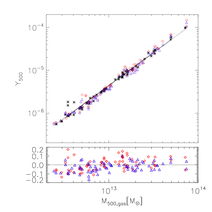
Figure 4.— Upper: Integrated Compton $y$ parameter inside $r_{500}$ from simulated clusters at z=0 epoch plotted against integrated mass inside the same radius. Stars are for the true values on the simulation grid, red diamonds represent values deduced by fitting to isothermal $\beta$-models, blue triangles are for fitting to a U-$\beta$ model. Lower: Log deviation of isothermal and U-$\beta$ points from the best-fit scaling relation for the true values.

On first inspection of Figure 4, it is not clear that either the isothermal or U-$\beta$ generates a more accurate result. The plot shows values from all clusters from the z=0 simulation epoch. The true values of $Y_{500}$ and $M_{500,gas}$ are plotted as stars, the isothermal model values as diamonds, and the U-$\beta$ model values as triangles.

The plot of deviation of these values from the best fit to the true values shows some difference between these two methods. However, it is important to remember that there are deviations from both the true integrated SZE, and the true gas mass, so these points deviate in both dimensions of the plot. Since errors in both are correlated, due to the dependence on the determination of $r_{500}$ from the $\beta$-model, this should reduce the apparent separation of points from the best fit, even when the values of both parameters are in error.

Figure 5.— Upper: Plot of the ratio of estimated $Y_{500}$ to its true value (y-axis) versus the ratio of estimated $M_{500,gas}$ to its true value for 493 simulated cluster projections for isothermal $\beta$-model fits. Lower: Ratio of estimated $Y_{500}$ to its true value versus the ratio of estimated $M_{500,gas}$ to its true value for U-$\beta$-model fits. Lines indicate location of perfectly accurate estimation of each quantity.

This important point is illustrated in Figure 5, which shows the the ratios of estimated to true values of $Y_{500}$ and $M_{500,gas}$ for each cluster. In both the isothermal (upper plot) and U-$\beta$ (lower plot) methods, there is a clear trend in over and underestimation in both values. These figures also illustrate nicely the improvement in values one gets with the U-$\beta$ method. The U-$\beta$ points are clustered more strongly around the correct values than are the isothermal estimates. This effect is illustrated in Figure 6, where we have plotted the true values of $y$ and $M$, with lines indicating the corresponding estimates of those values for the isothermal and U-$\beta$ methods. There are typically overestimates in both estimated $Y_{500}$ and $M_{500,gas}$, and the use of the U-$\beta$ typically brings the estimated values back toward the true.

The outliers in these plots are also interesting. The clusters which give strong overestimates of $Y$ and $M_{gas}$ typically result from line-of-sight overlap of multiple structures. This enhances the integrated SZE signal in projection, but overestimates the true value for the main cluster. The clusters with low estimated values of $Y$ and/or $M_{gas}$ typically have poor quality $\beta$-model fits (as measured by a $\chi^{2}$ statistic), and appear to have systematically low fitted values for the core radius. Some of these clusters appear to have weak cool cores, not meeting the cool core criteria, and thus were not excluded from the sample. It is interesting that the clusters with mass underestimates do not all generate underestimates of $Y$. This effect warrants further study.

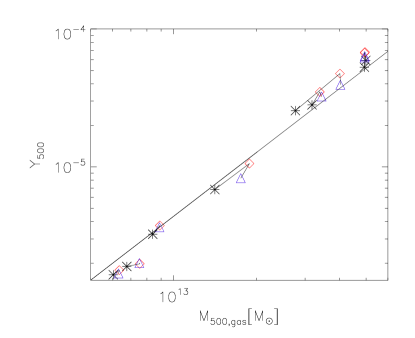
Figure 6.— Plot of eight clusters on the $Y_{500}$-$M_{500,gas}$ relation chosen to span a wide mass range, but otherwise randomly. Stars indicate the true values from the simulation, red diamonds the isothermal $\beta$-model estimates, and blue triangles the U-$\beta$ model estimates. Lines link points associated with the same cluster.

Table 3 also shows the result of this analysis. When using isothermal models, the median estimated value of $Y_{500}$ is 23% larger than the true value (the mean is a 28% overestimate). Additionally, when estimating the gas mass, the median estimated value is a 16% overestimate. In previous work (Hallman et al., 2006), we have shown that the magnitude of the overestimate via X-ray $\beta$-model methods is lower than this, but in that case we assumed one could correctly calculate the value of $r_{500}$ with no error. In either case, this overestimate is consistent with our previous work, and with that of others (Mohr et al., 1999; Mathiesen et al., 1999). The overestimate in mass results from substructure, merging and other physical processes not described by a simple model. In the current analysis, the value of $r_{500}$ is deduced directly from the $\beta$-model. In contrast, the U-$\beta$ method gets closer to the correct value for $Y_{500}$, with a median value 11% higher than the true value. For the mass, the U-$\beta$ method gets an estimate close to the true mass, a median overestimate of only 4%.

Additionally, using the U-$\beta$ method reduces the scatter in $Y_{500}$ values, as shown in Figure 7. The distribution of values is more sharply peaked, with a smaller high end tail in addition to a reduced bias compared to the isothermal method. In mass, the result is a reduced bias in the median values with a slight improvement in the scatter as shown in Figure 8.

Table 3Ratio of Estimated to True Values of Simulated Cluster Properties to $r_{500}$

	Isothermal	U-$\beta$
$\langle y_{500,est}/y_{500,true}\rangle$	1.28	1.13
$(y_{500,est}/y_{500,true}),median$	1.23	1.11
1$\sigma$ upper	1.50	1.24
1$\sigma$ lower	1.08	1.03
$\langle M_{500,gas,est}/M_{500,gas,true}\rangle$	1.17	1.05
$(M_{500,gas,est}/M_{500,gas,true}),median$	1.16	1.04
1$\sigma$ upper	1.31	1.18
1$\sigma$ lower	1.06	0.94

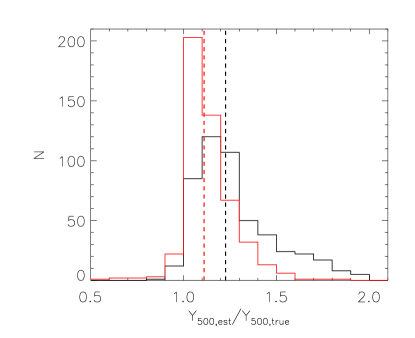
Figure 7.— Histogram of 493 simulated cluster projections of ratio of estimated $Y_{500}$ to true value for isothermal (black lines) and U-$\beta$ (red lines) methods. Dotted lines indicate median values for each distribution.

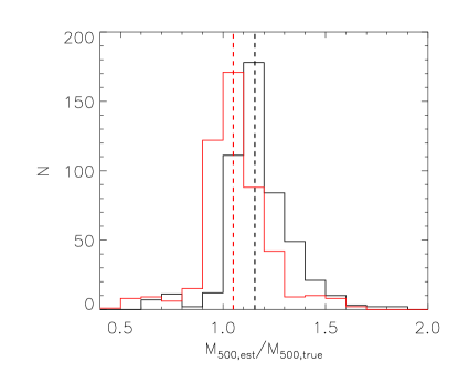
Figure 8.— Histogram of 493 simulated cluster projections of ratio of estimated $M_{500,gas}$ to true value for isothermal (black lines) and U-$\beta$ (red lines) methods. Dotted lines indicate median values for each distribution.

5. Conclusions

There is an inconsistency between X-ray and SZE fitted model parameters that leads to a bias in deduced values of $Y_{500}$ and $M_{500,gas}$ when using isothermal $\beta$-models. Using our U-$\beta$ model reduces the bias and scatter, resulting in a more precise and accurate determination of the $y$-$M$ scaling relation for clusters.

X-ray and SZE radial profiles from the same galaxy cluster can not be fit well by identical isothermal $\beta$-models. The stronger dependence of the SZE emission on temperature leads to problems when the cluster temperature declines with radius. In contrast, the strong dependence of the X-ray emission on density minimizes the error introduced by variations in cluster temperature. We show that fitting either the X-ray or SZE profiles to a modified, non-isothermal $\beta$-model corrected by the inclusion of a univeral temperature profile for clusters results in better consistency with the real values of $Y_{500}$ and $M_{500,gas}$.

We expect this inconsistency should affect measurements of the Hubble constant at some level, indeed it appears to result in a bias in $H_{0}$, as shown by Ameglio et al. (2006). There will certainly be an effect on gas fraction determinations, though it will also depend on any bias inherent in X-ray hydrostatic total mass estimates. While current precision in SZE/X-ray derived quantities is not high enough to reveal effects at the 10-20% level of the type described here, we expect it will be higher with larger samples and new instruments available in the near term. When contemplating clusters as precision cosmological tools, effects as this level must be considered.

While some have used double $\beta$-models (LaRoque et al., 2006) to fit cluster radial profiles with some success, a model like the U-$\beta$ is preferred, since it is physically motivated by the observed ICM properties. This work illustrates a simple modification of the isothermal $\beta$-model to more realistically account for cluster physics, and thus more accurately and precisely measure cluster properties.

Appendix A Derivation of UTP Surface Brightness Model

To derive a surface brightness model resulting from the UTP modified $\beta$-model, we take the standard $\beta$-model for density,

$$n_{e}(r)=n_{e0}\left(1+\left(\frac{r}{r_{c}}\right)^{2}\right)^{-3\beta/2},$$ (A1)

and the UTP model for temperature,

$$T(r)=\langle T\rangle_{500}T_{0}\left(1+\left(\frac{r}{\alpha r_{500}}\right)^{2}\right)^{-\delta},$$ (A2)

and substitute them into the integral of the X-ray surface brightness,

$$S_{X}(b)=\frac{1}{4\pi(1+z)^{4}}\int n_{e}(r)n_{H}(r)\Lambda(T(r))dl.$$ (A3)

In the simple bremsstrahlung case, $\Lambda(T)$ = $\Lambda_{0}T^{1/2}$. In that case,

$$S_{X}(b)=S_{X0}\left(1+\left(\frac{b}{r_{c}}\right)^{2}\right)^{-3\beta}\left(1+\left(\frac{b}{\alpha r_{500}}\right)^{2}\right)^{-\frac{\delta}{2}}I_{X}(b),$$ (A4)

where

$$S_{X0}=\frac{2{n_{e0}}^{2}\Lambda_{0}(\langle T\rangle_{500}T_{0})^{1/2}}{4\pi\kappa(1+z)^{4}},$$ (A5)

where $\kappa=\mu_{H}/\mu_{e}$, the ratio of the mean molecular weights of hydrogen and electrons. For $r_{c}<\alpha r_{500}$,

$$I_{X}(b)=\frac{r_{c}}{2}\left(1+\left(\frac{b}{r_{c}}\right)^{2}\right)^{1/2}B\left(\frac{1}{2},3\beta+\frac{\delta}{2}-\frac{1}{2}\right)F_{2,1}\left(\frac{\delta}{2},\frac{1}{2};3\beta+\frac{\delta}{2},1-\frac{{r_{c}}^{2}+b^{2}}{\alpha^{2}{r_{500}}^{2}+b^{2}}\right),$$ (A6)

where $F_{2,1}$ is Gauss’ hypergeometric function and $B$ is the Beta function defined by

$$B(x,y)=\frac{\Gamma(x)\Gamma(y)}{\Gamma(x+y)};x,y>0.$$ (A7)

For $r_{c}>\alpha r_{500}$,

$$I_{X}(b)=\frac{\alpha r_{500}}{2}\left(1+\left(\frac{b}{\alpha r_{500}}\right)^{2}\right)^{1/2}B\left(\frac{1}{2},3\beta+\frac{\delta}{2}-\frac{1}{2}\right)F_{2,1}\left(3\beta,\frac{1}{2};3\beta+\frac{\delta}{2},1-\frac{\alpha^{2}{r_{500}}^{2}+b^{2}}{{r_{c}}^{2}+b^{2}}\right).$$ (A8)

Similarly for the SZE, where

$$y=\int\sigma_{T}n_{e}(r)\frac{k_{b}T}{m_{e}c^{2}}dl,$$ (A9)

the substitution results in

$$y(b)=y_{0}\left(1+\left(\frac{b}{r_{c}}\right)^{2}\right)^{-\frac{3\beta}{2}}\left(1+\left(\frac{b}{\alpha r_{500}}\right)^{2}\right)^{-\delta}I_{SZ}(b),$$ (A10)

and

$$y_{0}=2\sigma_{T}n_{e0}\frac{k_{b}\langle T\rangle_{500}T_{0}}{m_{e}c^{2}}.$$ (A11)

For the two cases of $r_{c}<\alpha r_{500}$ and $r_{c}>\alpha r_{500}$ respectively,

$$I_{SZ}(b)=\frac{r_{c}}{2}\left(1+\left(\frac{b}{r_{c}}\right)^{2}\right)^{1/2}B\left(\frac{1}{2},\frac{3\beta}{2}+\delta-\frac{1}{2}\right)F_{2,1}\left(\delta,\frac{1}{2};\frac{3\beta}{2}+\delta,1-\frac{{r_{c}}^{2}+b^{2}}{\alpha^{2}{r_{500}}^{2}+b^{2}}\right),$$ (A12)

and

$$I_{SZ}(b)=\frac{\alpha r_{500}}{2}\left(1+\left(\frac{b}{\alpha r_{500}}\right)^{2}\right)^{1/2}B\left(\frac{1}{2},\frac{3\beta}{2}+\delta-\frac{1}{2}\right)F_{2,1}\left(\frac{3\beta}{2},\frac{1}{2};\frac{3\beta}{2}+\delta,1-\frac{\alpha^{2}{r_{500}}^{2}+b^{2}}{{r_{c}}^{2}+b^{2}}\right).$$ (A13)

Figure 9 shows the values for each of the line integrals as a function of projected radius normalized to $r_{500}$ for typical model parameters. We have created a calculator for the line integral in the Interactive Data Language (IDL), which is available on-line at http://solo.colorado.edu/ hallman/UTP/Ib_calc.tar.gz.

Figure 9.— Value of line integrals $I_{X}$ and $I_{SZ}$as a function of radius normalized to $r_{500}$. This calculation uses values near the mean of the distribution for all clusters for the $\beta$-model paramters, and $r_{500}$=1.0$h^{-1}$Mpc. $r_{core}$=160kpc, $\beta$=0.82, $\alpha$=1.15, $\delta$=0.5, therefore this is the case where $r_{core}<r_{500}$. Solid line is for X-ray integral, dotted is for SZE.

References

- Ameglio et al. (2006) Ameglio, S., Borgani, S., Diaferio, A., & Dolag, K. 2006, MNRAS, 369, 1459
- Bonamente et al. (2006) Bonamente, M., Joy, M. K., LaRoque, S. J., Carlstrom, J. E., Reese, E. D., & Dawson, K. S. 2006, ApJ, 647, 25
- Brickhouse et al. (1995) Brickhouse, N. S., Raymond, J. C., & Smith, B. W. 1995, ApJS, 97, 551
- Carlstrom et al. (2002) Carlstrom, J. E., Holder, G. P., & Reese, E. D. 2002, ARA&A, 40, 643
- Cavaliere & Fusco-Femiano (1978) Cavaliere, A. & Fusco-Femiano, R. 1978, A&A, 70, 677
- da Silva et al. (2000) da Silva, A. C., Barbosa, D., Liddle, A. R., & Thomas, P. A. 2000, MNRAS, 317, 37
- Hallman et al. (2006) Hallman, E. J., Motl, P. M., Burns, J. O., & Norman, M. L. 2006, ApJ, 648, 852
- Itoh & Nozawa (2004) Itoh, N. & Nozawa, S. 2004, A&A, 417, 827
- Joy et al. (2001) Joy, M., LaRoque, S., Grego, L., Carlstrom, J. E., Dawson, K., Ebeling, H., Holzapfel, W. L., Nagai, D., & Reese, E. D. 2001, ApJ, 551, L1
- Kravtsov et al. (2006) Kravtsov, A. V., Vikhlinin, A., & Nagai, D. 2006, ApJ, 650, 128
- LaRoque et al. (2006) LaRoque, S. J., Bonamente, M., Carlstrom, J. E., Joy, M. K., Nagai, D., Reese, E. D., & Dawson, K. S. 2006, ApJ, 652, 917
- Loken et al. (2002) Loken, C., Norman, M. L., Nelson, E., Burns, J., Bryan, G. L., & Motl, P. 2002, ApJ, 579, 571
- Mathiesen et al. (1999) Mathiesen, B., Evrard, A. E., & Mohr, J. J. 1999, ApJ, 520, L21
- Mohr et al. (1999) Mohr, J. J., Mathiesen, B., & Evrard, A. E. 1999, ApJ, 517, 627
- Motl & Burns (2005) Motl, P. M. & Burns, J. M. 2005, in X-Ray and Radio Connections (eds. L.O. Sjouwerman and K.K Dyer) Published electronically by NRAO, http://www.aoc.nrao.edu/events/xraydio Held 3-6 February 2004 in Santa Fe, New Mexico, USA, (E8.03) 8 pages
- Motl et al. (2004) Motl, P. M., Burns, J. O., Loken, C., Norman, M. L., & Bryan, G. 2004, ApJ, 606, 635
- Motl et al. (2005) Motl, P. M., Hallman, E. J., Burns, J. O., & Norman, M. L. 2005, ApJ, 623, L63
- Nagai (2006) Nagai, D. 2006, ApJ, 650, 538
- Nagai et al. (2000) Nagai, D., Sulkanen, M. E., & Evrard, A. E. 2000, MNRAS, 316, 120
- O’Shea et al. (2005) O’Shea, B. W., Bryan, G., Bordner, J., Norman, M. L., Abel, T., Harkness, R., & Kritsuk, A. 2005, in Adaptive Mesh Refinement: Theory and Applications (Berlin: Springer), 341
- Reese et al. (2002) Reese, E. D., Carlstrom, J. E., Joy, M., Mohr, J. J., Grego, L., & Holzapfel, W. L. 2002, ApJ, 581, 53
- Roettiger et al. (1996) Roettiger, K., Burns, J. O., & Loken, C. 1996, ApJ, 473, 651
- Sulkanen (1999) Sulkanen, M. E. 1999, ApJ, 522, 59
- Sunyaev & Zeldovich (1972) Sunyaev, R. A. & Zeldovich, Y. B. 1972, Comments on Astrophysics and Space Physics, 4, 173
- Vikhlinin et al. (2005) Vikhlinin, A., Markevitch, M., Murray, S. S., Jones, C., Forman, W., & Van Speybroeck, L. 2005, ApJ, 628, 655