Phase transition in the two-component symmetric exclusion process with open boundaries

Abstract

We consider single-file diffusion in an open system with two species $A,B$ of particles. At the boundaries we assume different reservoir densities which drive the system into a non-equilibrium steady state. As a model we use an one-dimensional two-component simple symmetric exclusion process with two different hopping rates $D_{A},D_{B}$ and open boundaries. For investigating the dynamics in the hydrodynamic limit we derive a system of coupled non-linear diffusion equations for the coarse-grained particle densities. The relaxation of the initial density profile is analyzed by numerical integration. Exact analytical expressions are obtained for the self-diffusion coefficients, which turns out to be length-dependent, and for the stationary solution. In the steady state we find a discontinuous boundary-induced phase transition as the total exterior density gradient between the system boundaries is varied. At one boundary a boundary layer develops inside which the current flows against the local density gradient. Generically the width of the boundary layer and the bulk density profiles do not depend on the two hopping rates. At the phase transition line, however, the individual density profiles depend strongly on the ratio $D_{A}/D_{B}$. Dynamic Monte Carlo simulation confirm our theoretical predictions.
Keywords: Driven diffusive systems (Theory), Exact results, Stochastic particle dynamics (Theory)

I Introduction

Single-file diffusion occurs when a random motion of particles is confined to a narrow channel where they cannot pass each other due to hard-core repulsion. Examples for this behaviour include molecules diffusing in the channels of certain zeolites Karg92 ; Kukl96 ; Keil00 , transport of colloidal spheres in one-dimensional channels Wei00 , or the dynamics of “defects” inside the “tube” to which entangled polymers are confined Perk94 . Also biological motors moving along macromolecules or microtubuli exhibit single-file motion, see e.g. Schu97 ; Lipo05 ; Nish05 and references therein. Single-file diffusion is an effectively one-dimensional many-body random process which exhibits intriguing correlation effects. It is known for a long time that the mean-square displacement of a tagged particle grows subdiffusively for late times with the square root of time Levi73 , see also vanB83 for an insightful theoretical derivation. Also macroscopic stationary properties in open systems, driven by an external gradient of the chemical potential shows interesting long-range correlations even if the interaction between particles is strictly local Spoh83 ; Derr02 ; Bert02 . This implies failure of Onsager theory and indicates strong non-equilibrium behaviour.

So far most theoretical treatments of single-diffusion have focussed on indistinguishable particles. The reference model for this process is the one-dimensional symmetric exclusion processes (SEP), a lattice model where hard-core particles hop randomly to nearest-neighbour sites, provided the target is empty Ligg99 ; Schu01 . However, already an experiment aimed at verifying the subdiffusive behaviour of a single tracer particle requires to tag one or more particles to make them distinguishable. This is done by labelling some particles without changing their diffusion properties and thus corresponds to a two-species SEP with identical hopping rates. A rigorous treatment of the macroscopic behaviour of such a two-component SEP with many tagged particles in terms of coupled non-linear diffusion equations for an infinite system was given by Quastel Quas92 . A finite system with open boundaries was treated only very recently Brza06 .

More generally, however, two physically distinct species of particles may simultaneously move inside the same channel. In recent measurements a mixture of toluene and propane was adsorbed into different zeolites Czap02 . The authors measured the temperature dependent outflow and noticed a trapping effect due to single-file diffusion: In zeolites with long intracrystalline channels the stronger adsorbed toluene molecules control due to blocking the outflow of propane. In terms of the SEP the different physical properties of toluene and propane require two different hopping rates. Also studying the drift velocity of an entangled polymer in gel electrophoresis in the framework of reptation theory necessitate a description of the defect dynamics in terms of two distinct species of particles Rubi87 ; Duke89 .

Somewhat surprisingly the hydrodynamic theory of two-component lattice gas models seems quite undeveloped even though there is some recent progress Toth03 ; Popk03b ; Schu03 . In Keil00 Keil et al. review the Maxwell-Stefan theory describing the diffusive behaviour of a binary fluid mixture where the total current, i.e. the sum of both species, is zero. The particle-particle interaction is taken into account by including a friction between the species being proportional to the differences in the velocities. However, this approach is purely phenomenological and does not provide a link between microscopic properties of the system and the transport coeffficients entering the macroscopic equation. In particular, this approach is not adequate for single-file diffusion in a finite system where the self-diffusivity of single particles has turned out to play an important role Brza06 .

In this paper we go beyond Ref. Brza06 by considering a two-component symmetric exclusion process with different hopping rates (defined in Sec. 2) and by studying not only stationary properties but also the time evolution of the particle density and relaxation towards the stationary state. To this end, generalizing the arguments put forward in Quas92 for identical particles, we consider open boundaries where both ends of the chain are connected to particle reservoirs with different chemical potentials. We derive in Sec. 3 a set of coupled nonlinear diffusion equations and we analyze the time-dependent solutions of these PDE’s by numerical integration. This is compared with simulation data obtained from dynamical Monte-Carlo simulations (DMCS) of the process. In Sec. 4 the stationary solution is obtained analytically in closed form and discussed in some detail. Some conclusions are drawn in Sec. 5. The exact computation of the self-diffusion coefficients for the two particle species is presented in the first appendix. The second appendix provides for self-containedness some technical details of that derivation.

II Two-component symmetric exclusion process

Following Brza06 we consider a one-dimensional lattice with $L$ lattice sites (Fig. 1). Each site $i$ can be empty or occupied by a particle of type $A$ or $B$. Due to hard-core interaction any site carries at most one particle. Particles can hop to nearest neighbour sites (provided the target site is empty) with hopping rates $D_{A/B}$ which are the “bare” diffusion coefficients, i.e., the proportionally factor in the mean-square displacement if no other particles were present. Jump events occur after an exponentially random time which in dynamic Monte Carlo simulations (DMCS) is modelled by random sequential update Brza06 .

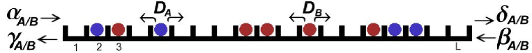
Figure 1: Two-component symmetric exclusion model with open boundaries. Each species of particles has its own hopping rates $D_{A},D_{B}$. At the boundaries particles are extracted and injected with rates as indicated.

Let $a_{i}$ ($b_{i}$) count the $A$ ($B$) particles on site $i$. Then the densities are the ensemble-averaged expectation values of the respective particle occupation numbers: $\left\langle a_{i}\right\rangle\equiv\rho_{A}(i)$, $\left\langle b_{i}\right\rangle\equiv\rho_{B}(i)$. The probability of finding no particle at site $i$ is $\left\langle v_{i}\right\rangle=\left\langle 1-a_{i}-b_{i}\right\rangle$. When we consider a chain with open boundary conditions, particles are injected and removed according to the boundary rates $\alpha_{A/B},\gamma_{A/B},\beta_{A/B}$ and $\delta_{A/B}$. So the attempt rate for an $A$-particle to enter the system at the left boundary is $\alpha_{A}$. It leaves the channel at the left boundary with rate $\gamma_{A}$ as illustrated in Fig. 1. The other boundary rates are defined similarly.

In terms of a quantum Hamiltonian formalism Schu01 the probability distribution of the system is represented by the probability vector $|P(t)>$ which evolves in time according to the master equation

$$\frac{d}{dt}|P(t)>=-H|P(t)>$$ (1)

where the generator $H$ has the structure

$$H=b_{1}+b_{L}+\sum_{i=1}^{L-1}h_{i,i+1}.$$ (2)

For an explicit representation of the generator we assign to the three allowed single-site states the three basis vectors

$$|A>\equiv|1>=\left(\begin{array}[]{l}1\\ 0\\ 0\end{array}\right),\quad|\emptyset>\equiv|0>=\left(\begin{array}[]{l}0\\ 1\\ 0\end{array}\right),\quad|B>\equiv|-1>=\left(\begin{array}[]{l}0\\ 0\\ 1\end{array}\right)$$ (12)

corresponding to having an $A$, no particle or $B$ at site $i$, respectively. A configuration of the full lattice is then represented by a tensor product of these basis vectors. To construct $H$, let $E_{k}^{x,y}$ be the $3\times 3$ matrix with one element located at column $x$ and row $y$ equal to one. All other elements are zero: $(E_{k}^{x,y})_{a,b}=\delta_{x,a}\delta_{y,b}$. The operator for annihilation (creation) of an $A$-particle at site $k$ is then $a_{k}^{-}=E_{k}^{1,2}$ ($a_{k}^{+}=E_{k}^{2,1}$) and for annihilation (creation) of $B$ is $b_{k}^{-}=E_{k}^{3,2}$ ($b_{k}^{+}=E_{k}^{2,3}$). Finally, the number operators are $a_{k}=E_{k}^{1,1}$, $b_{k}=E_{k}^{3,3}$, $v_{k}=1-a_{k}-b_{k}$. In this representation the boundary matrices are

$$b_{1}=\alpha_{A}(v_{1}-a_{1}^{+})+\alpha_{B}(v_{1}-b_{1}^{+})+\gamma_{A}(a_{1}-a_{1}^{-})+\gamma_{B}(b_{1}-b_{1}^{-})$$ (13)

$$b_{L}=\delta_{A}(v_{L}-a_{L}^{+})+\delta_{B}(v_{L}-b_{L}^{+})+\beta_{A}(a_{L}-a_{L}^{-})+\beta_{B}(b_{L}-b_{L}^{-}).$$ (14)

Hopping in the bulk between site $i$ and $i+1$ is generated by

$$h_{i,i+1}=D_{A}(a_{i}v_{i+1}+v_{i}a_{i+1}-a_{i}^{-}a_{i+1}^{+}-a_{i}^{+}a_{i+1}^{-})\\ +D_{B}(b_{i}v_{i+1}+v_{i}b_{i+1}-b_{i}^{+}b_{i+1}^{-}-b_{i}^{-}b_{i+1}^{+}).$$ (15)

The model is now well defined. We refer to appendix $A$ for more details on the formalism.

In Brza06 it was shown that with the choice $\frac{\alpha_{A}}{\gamma_{A}}=\frac{\delta_{A}}{\beta_{A}}\equiv\mu_{A}$ and $\frac{\alpha_{B}}{\gamma_{B}}=\frac{\delta_{B}}{\beta_{B}}\equiv\mu_{B}$ the process has an uncorrelated stationary equilibrium distribution with constant local particle densities

$$\rho_{A}=\frac{\frac{\alpha_{A}}{\gamma_{A}}}{1+\frac{\alpha_{A}}{\gamma_{A}}+\frac{\alpha_{B}}{\gamma_{B}}}=\frac{\frac{\delta_{A}}{\beta_{A}}}{1+\frac{\delta_{A}}{\beta_{A}}+\frac{\delta_{B}}{\beta_{B}}}$$ (16)

$$\rho_{B}=\frac{\frac{\alpha_{B}}{\gamma_{B}}}{1+\frac{\alpha_{A}}{\gamma_{A}}+\frac{\alpha_{B}}{\gamma_{B}}}=\frac{\frac{\delta_{B}}{\beta_{B}}}{1+\frac{\delta_{A}}{\beta_{A}}+\frac{\delta_{B}}{\beta_{B}}}.$$ (17)

Besides giving the equilibrium densities, these two equations above provide a recipe of how to translate the picture of inserting and deleting particles on boundary sites into a picture of constant reservoirs at the ends, see Fig. 2. One may regard the middle expression in (16) as a left reservoir density $\rho_{A}^{-}$ of $A$-particles, located at a virtual site $i=0$, with which the system exchanges particles by jump events with rates $D_{A,B}$. Similarly, the middle expression in (17) is a regarded as left reservoir density $\rho_{B}^{-}$ of $B$-particles. At the right boundary one adds a virtual reservoir (located at site $i=L+1$) with boundary densities $\rho_{A}^{+}$, $\rho_{B}^{+}$ given by the rightmost expressions in (16), (17).

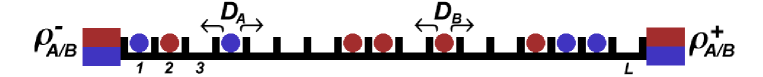
Figure 2: Three-state symmetric exclusion model with open boundaries – reservoir picture.

In this picture, jumping from a reservoir site onto the boundary of the system occurs proportional to the respective hopping rate and proportional to the single species boundary density. This parameterisation satisfies (16) and (17) if

$$\alpha_{A/B}=D_{A/B}\rho_{A/B}^{-},\quad\gamma_{A/B}=D_{A/B}(1-\rho_{A}^{-}-\rho_{B}^{-})$$ (18)

$$\delta_{A/B}=D_{A/B}\rho_{A/B}^{+},\quad\beta_{A/B}=D_{A/B}(1-\rho_{A}^{+}-\rho_{B}^{+}).$$ (19)

The second equality in (16), (17) is then the equilibrium condition $\rho_{A,B}^{-}=\rho_{A,B}^{+}$ of equal reservoir densities or chemical potentials $\mu_{A,B}^{-}=\mu_{A,B}^{+}$. In a non-equilibrium setting the left reservoir densities $\rho_{A}^{-}$, $\rho_{B}^{-}$ are not equal to those on the right boundary ($\rho_{A}^{+}$, $\rho_{B}^{+}$). In this boundary-driven case the system evolves towards a stationary state with non-vanishing particle currents.

Notice that for periodic boundary conditions the system is highly non-ergodic not only because of particle number conservation, but also because of the single-file constraint which conserves the sequence of particles. The open system, on the other hand, is ergodic because of the violation of the conservation of particles at the boundaries.

III Relaxation

III.1 Hydrodynamic limit

The average densities $\left\langle a_{i}\right\rangle$ and $\left\langle b_{i}\right\rangle$ satisfy the equations of motion $\frac{d}{dt}\left\langle a_{i}\right\rangle=-\left\langle a_{i}H\right\rangle$, $\frac{d}{dt}\left\langle b_{i}\right\rangle=-\left\langle b_{i}H\right\rangle$. This provides the Master equations for a single site,

$$\frac{d}{dt}\left\langle a_{i}\right\rangle =D_{A}\left(\left\langle a_{i-1}v_{i}\right\rangle+\left\langle a_{i+1}v_{i}\right\rangle-\left\langle a_{i}v_{i+1}\right\rangle-\left\langle a_{i}v_{i-1}\right\rangle\right)$$ (20)

$$\frac{d}{dt}\left\langle b_{i}\right\rangle =D_{B}\left(\left\langle b_{i-1}v_{i}\right\rangle+\left\langle b_{i+1}v_{i}\right\rangle-\left\langle b_{i}v_{i+1}\right\rangle-\left\langle b_{i}v_{i-1}\right\rangle\right).$$ (21)

At this stage we assume an infinite system and do not care about boundary sites. Nevertheless, in this form the equations of motion are not integrable. Replacing the joint probabilities by products of expectation values – according to a simple mean field ansatz which has been proven useful in other exclusion processes – fails to provide an even qualitatively correct description. However, an exact equation containing no correlators can be obtained from a weighted sum

$$\frac{d}{dt}\left(\frac{\left\langle a_{i}\right\rangle}{D_{A}}+\frac{\left\langle b_{i}\right\rangle}{D_{B}}\right)=\left(\left\langle a_{i-1}\right\rangle+\left\langle a_{i+1}\right\rangle-2\left\langle a_{i}\right\rangle+\left\langle b_{i-1}\right\rangle+\left\langle b_{i+1}\right\rangle-2\left\langle b_{i}\right\rangle\right).$$ (22)

of the individual particle densities.

The right-hand side contains a second-order difference for both species individually. Coarse-graining, i.e., replacing $i$ by the continuous variable $x=\frac{i}{a}$ and introducing $\rho_{A}(x,t)$, $\rho_{B}(x,t)$ as the $A$, $B$-particle density at $x$, transforms (22) (for vanishing lattice constant $a$) into the macroscopic equation

$$\partial_{t}\left(\frac{\rho_{A}(x,t)}{D_{A}}+\frac{\rho_{B}(x,t)}{D_{B}}\right)=\partial_{x}^{2}(\rho_{A}(x,t)+\rho_{B}(x,t)).$$ (23)

Here we used diffusive rescaling of the time-coordinate. Notice for the hydrodynamic limit (23) to be valid we implicitly use good local ergodic properties in the identification of the lattice expectation with the coarse-grained deterministc particle density. The weighted density on the l.h.s. of (23) and the total density on the r.h.s. reappear in the computations below and for notational simplicity we introduce

$$\rho(x,t)=\rho_{A}(x,t)+\rho_{B}(x,t)\sigma(x,t)=\frac{\rho_{A}(x,t)}{D_{A}}+\frac{\rho_{B}(x,t)}{D_{B}}$$ (24)

which reduces to $\sigma=\rho/D$ for equal single-particle diffusion coefficients $D_{A}=D_{B}\equiv D$.

The linear equation (24) does not provide a full description of the coarse-grained dynamics. To achieve this goal we generalize the approach of Quas92 and make an ansatz for the dynamics of a single particle (of species $A$ or $B$) localized at position $x$. This test particle acts as a tracer particle in the background of other particles, with a diffusive motion partially determined by its self-diffusion coefficient. Additionally, the test particle is subject to a background drift $b$ caused by the collective evolution of the entire system towards stationarity. A priori the self-diffusion coefficient for the two species of particles could be different. However, due to the single-file condition the long-time dynamics of a tracer particle is entirely determined by the background of other particles which is the same for both species. Hence we expect identical self-diffusion coefficients $D_{s}$ Asla00 . This physical picture leads us to the ansatz

$$\partial_{t}\rho_{A}(x,t) =\partial_{x}^{2}D_{s}\rho_{A}(x,t)-\partial_{x}b(x,t)\rho_{A}(x,t)$$ (25)

$$\partial_{t}\rho_{B}(x,t) =\partial_{x}^{2}D_{s}\rho_{B}(x,t)-\partial_{x}b(x,t)\rho_{B}(x,t).$$ (26)

for the time evolution of the coarse grained particle densities. The drift term $b$ can then be determined by using (23)

$$b=\frac{1}{\sigma}\partial_{x}(D_{s}\sigma-\rho).$$ (27)

In an infinite system the self-diffusion coefficient vanishes, as is indicated by the subdiffusive nature of single-file diffusion which was proved rigorously for tracer diffusion in the SEP in Arra83 . However, as argued in Brza06 we expect that in a finite system with open boundaries correction terms of leading order $1/L$ appear. This is confirmed by the exact result

$$D_{s}=\frac{1}{L}\frac{1-\rho}{\sigma}$$ (28)

derived in Appendix A for a periodic system. Introducing the two-component local order parameter

$$\vec{\rho}=\left(\begin{array}[]{l}\rho_{A}\\ \rho_{B}\end{array}\right)$$ (31)

finally leads to the coupled nonlinear diffusion equation

$$\partial_{t}\vec{\rho}=\partial_{x}\left(\hat{D}\partial_{x}\vec{\rho}\right)$$ (32)

with the diffusion matrix

$$\hat{D}=\frac{1}{\sigma}\left[\left(\begin{array}[]{cc}\rho_{A}&\rho_{A}\\ \rho_{B}&\rho_{B}\end{array}\right)+D_{s}\left(\begin{array}[]{cc}\frac{\rho_{B}}{D_{B}}&-\frac{\rho_{A}}{D_{B}}\\ -\frac{\rho_{B}}{D_{A}}&\frac{\rho_{A}}{D_{A}}\end{array}\right)\right].$$ (37)

This equation provides a complete description of the density dynamics in the hydrodynamic limit. For given initial density profiles the solution of (25), (26) is uniquely deternined. Notice that for an infinite system where $D_{s}=0$ the diffusion matrix $\hat{D}$ has a vanishing eigenvalue. For $D_{A}=D_{B}$ (25) and (26) reduce to the coupled nonlinear diffusion equations proved rigorously in Quas92 .

III.2 Time evolution of density profiles

We have no analytical expression for the solution of the system (32), but numerical integration can be performed to great accuracy using standard routines. We first study the case of equal hopping rates $D_{A}=D_{B}$. This case is similar to the tracer diffusion investigated in Kaerg2002 . Fig. 3 shows the penetration of tracer particles into the system with lattice size $L=200$ at four different times. Full lines are solutions of (32) obtained from numerical integration. Circles indicate the numerical DMCS densities. Initially, the lattice is prepared with a uniform distribution of $B$-particles and very few $A$-particles. The smooth drop of the initial $A$-particle profile at the edges was chosen for faster numerical integration. The boundary reservoir densities are $\rho_{A}^{-}=\rho_{A}^{+}=\rho_{B}^{-}=\rho_{B}^{+}=0.3$. For all instances of time the numerical integration shows a rather satisfying collapse with the profiles obtained from Monte Carlo simulation. Any DMCS in this work was averaged over at least 10000 realizations.

Figure 3: Density profiles of the $A$($B$)-component (upper/lower curve) at different MC times for a system ($L=200$) with equal diffusion coefficients. Snapshots are taken at a) $t=0$, b) $t=5000$, c) $t=50000$, d) $t=400000$. The system relaxes towards the equilibrium state given by the reservoir densities $\rho_{A/B}^{+/-}=0.3$. Symbols denote densities obtained from DMCS. Full lines come from numerical integration of the diffusion equation.

It is remarkable that the PDEs describe the intermediate flattening at the boundary (see e.g. Fig. 3c) of the $A$-particle profile which was observed for the first time in Kaerg2002 . It is also interesting that the spatial mean density of $B$-particles first grows before it relaxes to its equilibrium value 0.3. The explanation comes from the hydrodynamic equation (23) which states that the total density profile, i.e. the sum of both species, evolves according to an ordinary diffusion equation. Hence, the relaxation to equilibrium is proportional to $L^{2}$, in contrast to the much slower relaxation time of order $L^{3}$ of the individual components. The $B$-particles compensate the $A$-particle profile until both reach equilibrium.

As a second example we consider the relaxation of a mixed system with heavy $B$ particles and light $A$-particles where $D_{A}/D_{B}=5$. For Fig. 4 a)-c) we have chosen a model with $L=250$, and reservoir densities $\rho_{A}^{-}=\rho_{A}^{+}=\rho_{B}^{-}=\rho_{B}^{+}=0.3$ as before. The agreement between simulation and integration in the vicinity of the boundary is not as good as for tracer particles. Nevertheless, comparing the simulation results for the smaller lattice ($L=100$) shown in d) with the results for the larger lattice shown in c) suggests that the deviations are finite-size effects. We do not have a theory of finite-size effects beyond the leading $1/L$-correction to the self-diffusion coefficient. Therefore we do not pursue this issue further.

Figure 4: Snapshots of the density profiles for a system with $L=250$, $D_{A}/D_{B}=5$ and open boundary conditions with reservoir densities $\rho_{A/B}^{+/-}=0.3$. MC times are a) $t=0$, b) $t=10000$, c) $t=50000$. Circles denote densities obtained from DMCS. Full lines come from numerical integration of the hydrodynamic equation. The stronger discrepancy between simulation data and integration shown in Fig. d) for $L=100$ and $t=5000$ demonstrates significant finite size effects.

III.3 Small diffusion rate for one of the species

We discuss the case where one of the species, say $B$, is very heavy and has a vanishing hopping rate $D_{B}\to 0$. In this case even the open system is not ergodic and the stationary state to which the system relaxes depends on the initial distribution of $A$ and $B$-particles. $B$-particles just remain at their initial position and the equilibrium $A$-particle density between two $B$’s is just their local initial density. Let us now assume an initial state without any $B$-particles in the channel and let the reservoir densities be non-vanishing with $\rho_{A}=\rho_{A}^{-}=\rho_{A}^{+}$ and $\rho_{B}=\rho_{B}^{-}=\rho_{B}^{+}$. For the case of strictly vanishing hopping rate $D_{B}=0$ both injection rates of $B$-particles at the boundaries vanish and therefore no $B$-particles ever enter the system. Then the bulk dynamics follow the rules of the single-species SEP, but an anomaly comes from the fact that injection of $A$-particles is proportional to the $A$-particle density whereas the outgoing rate occurs according to the hole density which involves the reservoir density $\rho_{B}\neq 0$. Hence, $A$-particles do not equilibrate towards $\rho_{A}$ (as expected from the single-species SEP) but reach a higher value:

$$\rho^{D_{B}=0}_{A}=\frac{\alpha_{A}}{\alpha_{A}+\gamma_{A}}=\frac{\delta_{A}}{\delta_{A}+\beta_{A}}=\frac{\rho_{A}}{1-\rho_{B}}.$$ (38)

Notice that any ratio $\rho^{D_{B}=0}_{A}/\rho_{A}>1$ can be achieved provided $\rho_{B}$ and $D_{A}$ are large enough.

This leads to an interesting conclusion for small but non-vanishing $0<D_{B}\ll D_{A}/L^{2}$. Then channel is in a quasi-equilibrium with $A$-particles (with density (38)) before eventually a $B$-particle enters the system. Only very slowly both species start to relax to their common equilibrium state and one expects the $A$ profile to initially exceed its true equilibrium value $\rho_{A}$, up to some maximal value which is bounded by the maximal density (38). This overshooting is indeed observed in simulation, see Fig. 5 for the time evolution of the spatial mean densities. Initially the system ($L=50$) is almost empty and the particles are injected and removed at the boundaries according to the reservoir densities $\rho^{+/-}_{A/B}=0.3$. The ratio of the diffusion coefficient is $D_{A}/D_{B}=30$. One can clearly see the excess of $A$-particles which disappears only very slowly.

Figure 5: Mean density of $A$ and $B$-particles as a function of MC steps. The relaxation towards the equilibrium values $\rho_{A/B}^{+/-}=0.3$ was started from an almost empty lattice ($L=50$).

IV Steady state behaviour

IV.1 Finite $L$

In the steady state the time derivative in the diffusion equation (32) vanishes and from (23) we obtain the integration constant

$$\partial_{x}\rho=-c.$$ (39)

In terms of the individual stationary particle currents we have $c=j_{A}/D_{A}+j_{B}/D_{B}$. Integration yields the stationary total density profile $\rho=\rho_{A}+\rho_{B}$

$$\rho(x)=\rho^{-}+\frac{\rho^{+}-\rho^{-}}{L}x$$ (40)

in terms of the boundary values $\rho^{\pm}$. In terms of the boundary densities the integration constant is therefore given by

$$c=-\frac{\rho^{+}-\rho^{-}}{L}.$$ (41)

In order to compute the density profile of the $A$-species we introduce

$$h(x)\equiv\frac{\rho_{A}(x)}{\sigma(x)}=\frac{D_{B}\rho_{A}(x)}{\rho(x)-\left(1-\frac{D_{B}}{D_{A}}\right)\rho_{A}(x)}.$$ (42)

Given $h$ both $\rho_{A}$ and $\rho_{B}$ can be computed from (40). Using the self-diffusion coefficient (28), the stationarity condition for $\rho_{A}$ becomes

$$\frac{1}{L}\partial_{x}\left[(1-\rho)h\right]+\left(1+\frac{1}{L}\right)h\partial_{x}\rho=-j_{A}$$ (43)

with an integration constant $j_{A}$ proportional to the current of $A$-particles. Using the linearity of the total density profile this yields

$$\frac{1-\rho(x)}{L}h^{\prime}(x)-ch(x)+j_{A}=0.$$ (44)

where the prime denotes the derivative w.r.t. $x$.

This differential equation is straightforwardly integrated and one finds

$$h(x)=h^{-}-\frac{h^{-}-h^{+}}{1-\left(\frac{1-\rho^{+}}{1-\rho^{-}}\right)^{L}}\left[1-\left(1-\frac{\rho^{+}-\rho^{-}}{1-\rho^{-}}\frac{x}{L}\right)^{L}\right].$$ (45)

Here we have introduced the boundary value

$$h^{\pm}=\frac{\rho_{A}^{\pm}}{\frac{\rho_{A}^{\pm}}{D_{A}}+\frac{\rho_{B}^{\pm}}{D_{B}}}.$$ (46)

Solving for the density profile of $A$-particle then yields

$$\rho_{A}(x)=\left[\rho^{-}+(\rho^{+}-\rho^{-})\frac{x}{L}\right]\frac{h(x)}{D_{B}+\left(1-\frac{D_{B}}{D_{A}}\right)h(x)}.$$ (47)

The integration constant $j_{A}$ is given in terms of boundary densities by

$$j_{A}=\frac{h^{+}\left(1-\rho^{-}\right)^{L}-h^{-}\left(1-\rho^{+}\right)^{L}}{\left(1-\rho^{-}\right)^{L}-\left(1-\rho^{+}\right)^{L}}\frac{\rho^{-}-\rho^{+}}{L}.$$ (48)

Generically this quantity is of order $1/L$, up to corrections which are exponentially small in system size as long as $\rho^{-}\neq\rho^{+}$.

For vanishing reservoir gradient $\rho^{+}=\rho^{-}\equiv\rho$ we have $c=0$. This yields a linear function

$$h(x)=h^{-}-(h^{-}-h^{+})\frac{x}{L}$$ (49)

and nonlinear density profile

$$\rho_{A}(x)=\frac{\rho_{A}^{-}\left[1-\left(1-\frac{D_{B}}{D_{A}}\right)\frac{\rho_{A}^{+}}{\rho}\right]+\left(\rho_{A}^{+}-\rho_{A}^{-}\right)\frac{x}{L}}{1-\left(1-\frac{D_{B}}{D_{A}}\right)\frac{\rho_{A}^{+}}{\rho}+\left(1-\frac{D_{B}}{D_{A}}\right)\frac{\rho_{A}^{+}-\rho_{A}^{-}}{\rho}\frac{x}{L}}.$$ (50)

The current of $A$-particles

$$j_{A}=\frac{1-\rho}{L^{2}}\left(h^{-}-h^{+}\right)$$ (51)

is only of order $1/L^{2}$, as opposed to the generic $1/L$ dependence. For the total particle current we find

$$j\equiv j_{A}+j_{B}=\frac{\rho(1-\rho)}{L^{2}}\frac{\left(\rho_{A}^{+}-\rho_{A}^{-}\right)\left(D_{A}^{-1}-D_{B}^{-1}\right)}{\sigma^{+}\sigma^{-}}=\frac{\rho}{L}(D_{s}^{-}-D_{s}^{+})$$ (52)

which is also of order $1/L^{2}$. We remark that this current is proportional to the boundary gradient of the self-diffusivity.

IV.2 Phase transition in the thermodynamic limit

The expression for the $A$-particle density derived for finite $L$ is cumbersome. Rather interesting behaviour emerges from an analysis of the thermodynamic limit $L\to\infty$. To leading order in $1/L$ we find

$$j_{A}=\left\{\begin{array}[]{ll}\frac{\rho_{A}^{+}}{\frac{\rho_{A}^{+}}{D_{A}}+\frac{\rho_{B}^{+}}{D_{B}}}\frac{\rho^{-}-\rho^{+}}{L}&\mbox{ for }\rho^{-}<\rho^{+}\\ \frac{\rho_{A}^{-}}{\frac{\rho_{A}^{-}}{D_{A}}+\frac{\rho_{B}^{-}}{D_{B}}}\frac{\rho^{-}-\rho^{+}}{L}&\mbox{ for }\rho^{-}>\rho^{+}\end{array}\right.$$ (55)

Hence, as one expects, the $A$-current is always opposite the total reservoir gradient $\Delta\rho\equiv\rho^{+}-\rho^{-}$, but it changes in a non-analytic fashion at $\rho^{-}=\rho^{+}$ where it vanishes to leading order in $1/L$, see (51). For positive reservoir gradient $\Delta\rho$ the amplitude of $A$-current is governed by the reservoir density at right boundary, otherwise by the left boundary.

A nonanalyticity at $\Delta\rho=0$ appears also in the behaviour of the density. Using $\lim_{L\to\infty}(1-ax/L)^{L}={\rm e}^{-ax}$ yields the following behaviour.

Case 1, $\rho^{-}<\rho^{+}$: Straightforward algebra turns (45) into

$$h(x)=h^{+}+(h^{-}-h^{+}){\rm e}^{-x/\xi}$$ (56)

with localization length

$$\xi=\left[\ln{\frac{\rho^{+}-\rho^{-}}{1-\rho^{-}}}\right]^{-1}.$$ (57)

This gives

$$\rho_{A}(x)=\left[\rho^{-}+(\rho^{+}-\rho^{-})\frac{x}{L}\right]\frac{h^{+}+(h^{-}-h^{+}){\rm e}^{-x/\xi}}{D_{B}+\left(1-\frac{D_{B}}{D_{A}}\right)\left[h^{+}+(h^{-}-h^{+}){\rm e}^{-x/\xi}\right]}.$$ (58)

For large distance $x\gg\xi$ from the left boundary the function $h$ approaches a constant and the density profile of $A$-particles becomes proportional to the total density

$$\rho_{A}(x)\to\frac{\rho_{A}^{+}}{\rho^{+}}\rho(x).$$ (59)

Therefore at large distance from the boundary the density of each species becomes a linear function. The exponentially decaying deviation from linearity marks the occurrence of a boundary layer of width $\xi$ at the left boundary. Boundary layers in two-component systems with open boundaries were previously observed in Brza06 ; Vase06 and in earlier work Kaerg2002 ; Leeuwen2003 . The asymptotic space-averaged mean density

$$\bar{\rho}_{A}=\lim_{L\to\infty}\frac{1}{L}\int_{0}^{L}dx\rho_{A}(x)$$ (60)

takes the value

$$\bar{\rho}_{A}=\frac{\rho_{A}^{+}}{\rho^{+}}\frac{\rho^{+}+\rho^{-}}{2}$$ (61)

which is independent of $D_{B}/D_{A}$.

Case 2, $\rho^{-}>\rho^{+}$: The computation for negative reservoir gradient $\Delta\rho<0$ is analogous and all results can be obtained from Case 1 by interchanging $(+,-)$ and $(x,L-x)$. One finds

$$h(x)=h^{-}-(h^{-}-h^{+}){\rm e}^{-(L-x)/\xi}$$ (62)

with localization length

$$\xi=\left[\ln{\frac{\rho^{-}-\rho^{+}}{1-\rho^{+}}}\right]^{-1}.$$ (63)

This corresponds to a boundary layer at the right boundary of the system. For large distance $L-x\gg\xi$ from the right boundary the function $h$ approaches a constant and the the density profile of $A$-particles becomes proportional to the total density

$$\rho_{A}(x)\to\frac{\rho_{A}^{-}}{\rho^{-}}\rho(x)$$ (64)

Correspondingly one has

$$\bar{\rho}_{A}=\frac{\rho_{A}^{-}}{\rho^{-}}\frac{\rho^{+}+\rho^{-}}{2}$$ (65)

Therefore the mean density as a function of the reservoir gradient $\Delta\rho$ has a jump discontinuity at $\Delta\rho=0$. In each of the two phases it is controlled by the boundary which does not exhibit the boundary layer.

V Conclusions

The paper is dedicated to a detailed quantitative investigation single-file diffusion with two species of particles in an open system. Adapting ideas from the probabilistic hydrodynamic approach and using information from the microscopic master equation lead us to derive a nonlinear diffusion equations for the evolution of the macroscopic particle densities. We compute the exact self-diffusion coefficients $D_{s}$ for the two species which are equal and of order $1/L$. Hence they vanish in the hydrodynamic limit, in agreement with the subdiffusive behaviour of single-file diffusion. However, setting $D_{s}=0$ renders the diffusion matrix singular (with a vanishing eigenvalue) and the boundary-value problem becomes overdetermined. Therefore we conclude that $D_{s}$ is required for regularization. By use of numerical integration and Monte Carlo simulation the relaxation for the two species towards equilibrium is analysed. The very slow relaxation of the individual particle species is affected by a fast relaxation of the sum of both species. The density of the fast species reaches a maximum before it starts to relax slowly to its actual equilibrium value. From the diffusive nature of the collective behaviour we conclude that the collective relaxation time is of order $L^{2}$. The $1/L$-behaviour of the self-diffusion coefficient then implies single-species relaxation times of order $L^{3}$.

The diffusion equations are solved analytically for the stationary case. There is a boundary-induced non-equilibrium phase transition of first order. This transition resembles a similar transition observed in previous work Brza06 in so far as (i) this transition occurs when there is no gradient in the reservoir densities $\rho^{+},\rho^{-}$ and (ii) the transition is accompanied by a discontinuous change of the position of the boundary layer from one boundary to the other. However, a detailed analysis of our results reveals some interesting new features. Neither the width of the boundary layer nor the stationary bulk density profiles (59) depend on the ratio $D_{B}/D_{A}$ inside the two phases. At the phase transition line $\Delta\rho=0$, however, the individual density profiles are strongly sensitive to the ratio $D_{B}/D_{A}$. Unlike in the case of equal hopping rates the total particle current $j$ does not vanish, even though the total density $\rho=\rho_{A}+\rho_{B}$ is constant and equal to the reservoir densities. In terms of currents the phase transition occurs when the weighted current $c=j_{A}/D_{A}+j_{B}/D_{B}$ vanishes.

Boundary layers are known to occur also in bulk-driven lattice gases and have been analyzed in some detail in a series of recent papers Anta00 ; Popk03a ; Rako03 . They arise as a consequence of short-range correlations or because of the occurrence of shocks. They have a microscopic width which is finite on lattice scale and hence leads to a boundary discontinuity when under hydrodynamic scaling the lattice spacing is sent to zero. This is contrast to the boundary layers observed here which remains finite even for vanishing lattice spacing. Since there are no shocks in purely boundary-driven system, a possible explanation for the origin of the boundary layers could be the presence of long-range correlations in the stationary distribution.

Acknowledgement: Financial support by the Deutsche Forschungsgemeinschaft within the priority programme SPP1155 is gratefully acknowledged. We also thank Rosemary Harris, Dragi Karevski, Jörg Kärger and Henk van Beijeren for useful discussions. G.M.S thanks the Isaac Newton Institute for Mathematical Sciences (Cambridge), where part of this work was done, for kind hospitality.

Appendix A Exact two-species self-diffusion coefficients on a finite lattice

The self-diffusion coefficient is defined to be proportional to the asymptotic variance of the displacement $x(t)$. More precisely, we define

$$D_{s}=\frac{1}{2}\lim_{t\to\infty}\frac{d}{dt}\left(\left\langle x^{2}\right\rangle-\left\langle x\right\rangle^{2}\right).$$ (66)

of a tagged particle in infinite space. For an equilibrium system not driven by external forces one has $\left\langle x\right\rangle=0$ and the variance reduces to the mean square displacement $\left\langle x^{2}\right\rangle$. For finite time one cannot generally expect $D_{s}$ to be constant (anomalous diffusion), in particular for single-file systems with one species of particles $D_{s}$ vanishes asymptotically as $t^{-\frac{1}{2}}$, see Levi73 ; vanB83 , and for a mathematically rigorous proof for the SEP Arra83 .

For a finite system defined on a ring with periodic boundary conditions the definition (66) becomes meaningless. For a lattice model we consider instead the number of jumps $x^{+}$ in “positive” direction (say, clockwise) and the number of jumps $x^{-}$ in the opposite direction. As displacement we then define the quantity $x=x^{+}-x^{-}$. The diffusion coefficient may then be defined by (66). In a periodic single-file system with $L$ sites $D_{s}$ is finite even for $t\to\infty$ and is proportional to $1/L$ vanB83 . In the two-component symmetric simple exclusion process we one at first sight sight expect two different self-diffusion coefficients $D_{sA}$ and $D_{sB}$ for the $A$ and $B$ particles, respectively. In this section we show that $D_{sA}=D_{sB}\equiv D_{s}$ by an exact calculation for $t\to\infty$ for a finite system with periodic boundary conditions. The calculation is done via a mapping of the exclusion process to the zero range process (ZRP) as follows.

In the lattice gas picture the state of the system with length $L$ is characterized by a set of $L$ occupation numbers $y=(y_{1},...,y_{L})$ each of which can take values $-1$ (B-particle), $1$ (A-particle) or $0$ (vancancy). One defines a different lattice by labelling the $N$ particles as illustrated in Fig. 6. The individual labels correspond to the site number of the new lattice which, therefore, is of length $N$. Let $s=(s_{1},...,s_{N})$ be the configuration of the new lattice. Then $s_{i}=0,1,2,..$, counting the number of particles at site $i$ is defined as the number of empty sites to the right of particle $i$ in the SEP. This yields a particle system without exclusion, named zero range process (ZRP) Spit70 . A jump of particle $i$ in the SEP to the right induces a jump of a particle located on site $i$ of the ZRP to site $i-1$. Similarly, a jump to the left in the SEP corresponds to a jump from $i-1$ to $i$ in the ZRP. The different hopping rates $D_{A}$, $D_{B}$ assigned to a particle in the SEP are translated into different hopping rates across bonds in the ZRP. The symmetry in hopping of the SEP is translated into a symmetric hopping across a bond.

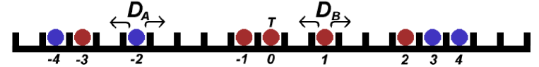
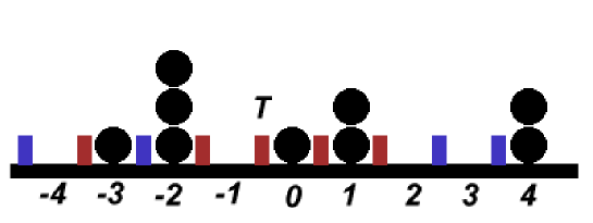
Figure 6: Mapping of the SEP with two species of particles to the ZRP. Particles in the SEP correspond to sites in the ZRP and interparticle distances correspond to occupation numbers. The particle hopping rate in the SEP maps to a hopping rate across bonds as indicated.

In order to proceed with the calculation of the $A$-particle self-diffusion coefficient we tag an $A$-particle and without loss of generality label it by zero. Let us now track the displacement of this particle set $x(0)=0$. Then the displacement $x(t)$ for the particle located on the ring is the number of jumps to the left minus the number of jumps to the right, performed within the time span 0 and t. In terms of the ZRP this number corresponds to the total particle current across bond $(0,1)$. The location of a tagged particle is thus given by counting the number of jumps across a fixed bond in the ZRP.

In order to set up the generator for the ZRP we define the single-site basis vectors for site $i$ as follows: An infinite row vector with a ’$1$’ at the first entry (zero elsewhere) is assigned to having no particle at site $i$. Provided site $i$ carries one particle, then a vector with ’$1$’ at the second entry (zero elsewhere) is assigned and so on. The basis vectors for the entire chain are as usual composed by a tensor product of the single-site vectors. $A$ hopping event from site $i$ to $i+1$ is described by the combined action of the creation and annihilation matrix $a^{+}_{i+1}$ and $a^{-}_{i}$. See appendix $B$ for a representation of the matrices and details of the calculation. To each bond $(i-1,i)$ we need to assign a hopping rate $D_{i}=(D_{A},D_{B})$ which corresponds to the hopping rate of the $i$’th particle in the SEP. This yields the following expression for the Hamiltonian:

$$H_{ZRP}=-\sum_{i}D_{i}\left(a_{i}^{-}a_{i+1}^{+}-d_{i}+a_{i}^{+}a_{i+1}^{-}-d_{i+1}\right)$$ (67)

The diagonal part of the Hamiltonian which ensures conservation of probability is constructed by the operators $d_{i}$. We remind the reader that the ground state of this Hamiltonian gives the stationary probability distribution which is unique for given total number of particles in the zero-range process.

For purposes that will immediately become clear we also introduce a non-equilibrium ZRP where particle hopping across bond $(0,1)$ is asymmetric, i.e., a particle hops from site 0 to site 1 with a rate $D_{A}q$ and with rate $D_{A}q^{-1}$ it hops from site 1 to site 0. Notice that due to periodic boundary conditions site 0 is identical with site $N$. We set $q={\rm e}^{E/2}$ where $E$ plays the role of a local driving force (measured in units of the thermal factor $k_{B}T$). The generator of this driven process may be written

$$H_{ZRP}(E)=H_{ZRP}+V(E)$$ (68)

where

$$V(E)=V=-D_{A}(q-1)(a_{0}^{-}a_{1}^{+}-d_{0})-D_{A}(q^{-1}-1)(a_{0}^{+}a_{1}^{-}-d_{1}).$$ (69)

In this system a stationary current $j(E)$ will emerge. In the original SEP this modification corresponds to a force acting on the tagged particle. The Einstein relation Katz84 then asserts that

$$D_{s}=j^{\prime}(0)$$ (70)

where the prime denotes the derivative w.r.t. the force $E$.

The proof of this relation Katz84 does not seem to be generally known and we outline the main ideas here. In order to track the number of jumps over bond $(-1,0)$ we follow the strategy of Gabi2004 and introduce the counting operators $X^{+}$ and $X^{-}$, counting clockwise and anticlockwise jumps, see also Harr07 for a more general description of counting processes. The counting operators act locally on an additional subspace with the action

$$X_{-}|k> =|k-1>$$ (71)

$$X_{+}|k> =|k+1>.$$ (72)

Tracking the position of the tagged particle in the SEP is now implemented by the operator $X$ with eigenvalue $k$: $X|k>=k|k>$. The full Hamiltonian $H=H_{ZRP}+V$ may be split into a term $H_{ZRP}$, and a “perturbation” $V$ with $V=-D_{A}(X^{+}-1)a_{0}^{-}a_{1}^{+}-D_{A}(x^{-}-1)a_{0}^{+}a_{1}^{-}$.

Due to the left-right symmetry of the hopping, $\left\langle x(t)\right\rangle=0$. It remains to calculate the second moment of the displacement $x$ in the late-time limit

$$\left\langle x^{2}\right\rangle=\left\langle s|X^{2}e^{-Ht}|P^{*}\right\rangle.$$ (73)

where $|P^{*}\rangle$ is the stationary probability vector. This computation starts by expanding the exponential $\exp(-Ht)$ into a time-ordered Dyson series with respect to the perturbation $V$

$$e^{-(H_{ZRP}+V)t}=e^{-H_{ZRP}t}\left[1-\int_{0}^{t}d\tau_{1}V(\tau_{1})+\int_{0}^{t}d\tau_{1}\int_{0}^{\tau_{1}}d\tau_{2}V(\tau_{1})V(\tau_{2})-...\right]$$ (74)

with $V(\tau)=e^{H_{ZRP}\tau}Ve^{-H_{ZRP}\tau}$. When calculating the $n$’th moment of $x$ any terms of order than higher $n$ vanish identically in the matrix element (73) which follows from the commutation relation $[X,X^{\pm}]=\pm X^{\pm}$ and $\langle s|X^{\pm}=\langle s|$.

$$<x^{2}>=-<s|X^{2}e^{-H_{ZRP}t}\int_{0}^{t}d\tau_{1}V(\tau_{1})|P^{*}>\\ +<s|x^{2}e^{-H_{ZRP}t}\int_{0}^{t}d\tau_{1}\int_{0}^{\tau_{1}}d\tau_{2}V(\tau_{1})V(\tau_{2})|P^{*}>$$ (75)

and one finds

$$D_{s}=D_{A}\lim_{t\to\infty}\left(\frac{D_{A}}{2}\left(\left\langle d_{0}\right\rangle+\left\langle d_{1}\right\rangle\right)-D_{A}\int_{0}^{\infty}dt\left\langle s|(d_{0}-d_{1})e^{-Ht}(d_{0}-d_{1})|P^{*}\right\rangle\right).$$ (76)

The proof of the Einstein relation (70) is completed by noting that the same expression involving the time-integrated current-correlation function appears in the computation of $j^{\prime}(0)$ using standard first-order time-dependent perturbation theory from quantum mechanics.

For the actual computation of $D_{s}$ we therefore need $j(E)$ which is computed in the next appendix. From (117) we read off by taking the derivative at $E=0$

$$D_{s}=z_{0}\left[\sum_{i=1}{M-1}{D_{i}^{-1}}\right]^{-1}$$ (77)

Using $M=N_{A}+N_{B}$ and (118) this yields in terms of the parameters of the two-component SEP

$$\sum_{i=1}{M-1}{D_{i}^{-1}}=\frac{1}{L}\left(\frac{\rho_{A}}{D_{A}}+\frac{\rho_{B}}{D_{B}}\right)$$ (78)

from which (28) follows.

Appendix B Quantum Hamiltonian formalism for the zero-range process

The state of a single site $i$ is characterized by the occupation number $s_{i}$. Let us first confine to the case of non-conserved particle number. For the infinite number of states one chooses the vector representation with the single-site basis vectors

$$|0>=\left(\begin{array}[]{l}1\\ 0\\ 0\\ \vdots\end{array}\right),\quad|1>=\left(\begin{array}[]{l}0\\ 1\\ 0\\ \vdots\end{array}\right),\quad|2>\left(\begin{array}[]{l}0\\ 0\\ 1\\ \vdots\end{array}\right).$$ (91)

The basis vectors representing the state of the entire lattice with $M$ is given by the tensor product of the single-site vectors

$$|\eta>=|s_{0}>\otimes|s_{1}>\otimes...\otimes|s_{M-1}>.$$ (92)

In this basis the operation of creating ($a_{i}^{+}$) and deleting a particle ($a_{i}^{-}$) at site $i$ is represented by the matrices

$$a_{i}^{+}=\left(\begin{array}[]{lllll}0&&&&\\ 1&\ddots&&&\\ &\ddots&\ddots&&\\ &&1&0&\\ &&&\ddots&\ddots\end{array}\right)\quad a_{i}^{-}=\left(\begin{array}[]{lllll}0&1&&&\\ &\ddots&\ddots&&\\ &&\ddots&1&\\ &&&0&\ddots\\ &&&&\ddots\end{array}\right)$$ (103)

The operator $a_{i}^{+}a_{i+1}^{-}$, hence, describes hopping from site $i+1$ to $i$. According to the rules described in appendix A, conservation of probability demands to introduce

$$d_{i}=\left(\begin{array}[]{lll}0&&\\ &1&\\ &&\ddots\\ \end{array}\right).$$ (107)

The stationary state for $H_{ZRP}$ (67) can be obtained by a product ansatz of the form

$$|P^{*}>=(1-z)\left(\begin{array}[]{l}1\\ z\\ z^{2}\\ \vdots\end{array}\right)^{\otimes M}$$ (112)

where the fugacity $z$ is related to the ZR particle density via $z=\frac{c}{1+c}$. For space-dependent hopping rates the same ansatz works with space-dependent fagacity $z_{i}$. This fugacity is determined by the stationarity condition

$$H|P^{*}>=0$$ (113)

which together with

$$\left\langle d_{i}\right\rangle=z_{i}$$ (114)

yields the recursion relation

$$j=D_{i}(z_{i}-z_{i+1})\quad i\neq 0$$ (115)

$$=D_{0}(qz_{0}-q^{-1}z_{1}).$$ (116)

Here we have assumed periodic boundary conditions with site $M\equiv 0$.

This recursion is solved in terms of the free parameter $z_{0}$ by the relation

$$j=z_{0}\frac{q-q^{-1}}{D_{0}^{-1}+q^{-1}\sum_{i=1}^{M-1}D_{i}^{-1}}.$$ (117)

The fugacity $z_{0}$ fixes the local density at site $i=0$ and via (114) all other local densities. We remark that $z_{k}-z_{1}=j\sum_{i=1}{k-1}{D_{i}^{-1}}$ which by the law of large numbers implies a linear fugacity profile on macroscopic scale. For $q=1$ (vanishing driving field $E=0$) we have $j=0$ and therefore constant fugacities $z_{k}=z=c/(1+c)$. In terms of the particle density in the underlying SEP with $N=M$ particles this gives

$$z=1-\rho.$$ (118)

References

- (1) Kärger J and Ruthven D M 1992 Diffusion in zeolites (John Wiley: New York)
- (2) Kukla V, Kornatowski J, Demuth D, Girnus I, Pfeifer H, Rees L V C, Schunk S, Unger K and Kärger J 1996 NMR studies of single-file diffusion in unidimensional channel zeolites Science 272 702
- (3) F. Keil, R. Krishna, M.-O. Coppens 2000 Modeling of diffusion in zeolites Rev. Chem. Eng. 16 71
- (4) Wei Q-H, Bechinger C and Leiderer P 2000 Single-File diffusion of colloids in one-dimensional channels Science 287 625
- (5) Perkins T T, Smith D E and Chu S 1994 Direct observation of tube-like motion of a single polymer-chain Science 264 819
- (6) Schütz G M 1997 The Heisenberg chain as a dynamical model for protein synthesis - Some theoretical and experimental results Int. J. Mod. Phys. B 11 197
- (7) Lipowsky R and Klumpp S 2005 ’Life is motion’: multiscale motility of molecular motors Physica A 352(1) 53
- (8) Nishinari K, Okada Y, Schadschneider A and Chowdhury D 2005 Intracellular transport of single-headed molecular motors KIF1A Phys. Rev. Lett. 95 118101.
- (9) Levitt D G 1973 Dynamics of a Single-File Pore: Non-Fickian Behavior Phys. Rev. A 8 3050
- (10) van Beijeren H, Kehr K W and Kutner R 1983 Diffusion in concentrated lattice gases. III. Tracer diffusion on a one-dimensional lattice Phys. Rev. B 28 5711
- (11) Spohn H 1983 Long-range correlations for stochastic lattice gases in a non-equilibrium steady state J. Phys. A 16 4275
- (12) Derrida B, Lebowitz J L, and Speer E R 2002 Large deviation of the density profile in the steady state of the open symmetric simple exclusion process J. Stat. Phys. 107 599
- (13) Bertini L, De Sole A, Gabrielli D, Jona-Lasinio G and Landim C 2002 Macroscopic fluctuation theory for stationary non-equilibrium states J. Stat. Phys. 107 635
- (14) Liggett T M 1999 Stochastic Models of Interacting Systems: Contact, Voter and Exclusion Processes (Berlin: Springer)
- (15) Schütz G M 2001 Exactly solvable models for many-body systems far from equilibrium, in: Phase Transitions and Critical Phenomena. Vol. 19, eds C Domb and J Lebowitz (London: Academic Press)
- (16) Quastel J 1992 Diffusion of Color in the simple exclusion process Comm. Pure Appl. Math. 45 623
- (17) Brzank A and Schütz G M 2006 Boundary-induced bulk phase transition and violation of Fick’s law in two-component single-file diffusion with open boundaries Diffusion Fundamentals 4 7.1-7.12
- (18) Czaplewski K F, Reitz T L, Kim Y J and Snurr R Q 2002 One-dimensional zeolites as hydrocarbon traps Micropor. Mesopor. Mater. 56 55
- (19) Rubinstein M 1987 Discretized model of entangled-polymer dynamics Phys. Rev. Lett. 59 1946
- (20) Duke T A J 1989 Tube model of field-inversion electrophoresis Phys. Rev. Lett. 62 2877
- (21) Toth B and Valko B 2003 Onsager relations and Eulerian hydrodynamic limit for systems with several conservation laws J. Stat. Phys. 112(3-4) 497
- (22) Popkov V and Schütz G M Shocks and excitation dynamics in a driven diffusive two-channel system J. Stat. Phys. 112(3-4) 523
- (23) Schütz G M 2003 Critical phenomena and universal dynamics in one-dimensional driven diffusive systems with two species of particles J. Phys. A 36 R339
- (24) Aslangul C 2000 Single-file diffusion with random diffusion constants J. Phys. A 33 851
- (25) Arratia R 1983 The Motion of a Tagged Particle in the Simple Symmetric Exclusion System in Z Ann. Prob. 11 362
- (26) Vasenkov S, Schüring A and Fritzsche S 2006 Single-file diffusion near channel boundaries Langmuir 22 5728
- (27) Vasenkov S and Kärger J Different time regimes of tracer exchange in single-file systems Phys. Rev. E 66 052601
- (28) Drzewinski A, Carlon E and van Leeuwen J M J 2003 Pulling reptating polymers by one end: Magnetophoresis in the Rubinstein-Duke model Phys. Rev. E 68 061801
- (29) Antal T and Schütz G M 2000 Asymmetric exclusion process with next-nearest-neighbor interaction: Some comments on traffic flow and a nonequilibrium reentrance transition Phys. Rev. E 62 83
- (30) Popkov V, Rákos A, Willmann R D, Kolomeisky A B and Schütz G M 2003 Localization of shocks in driven diffusive systems without particle number conservation Phys. Rev. E 67 066117 Part 2 JUN 2003
- (31) Rakos A, Paessens M and Schütz G M 2003 Hysteresis in one-dimensional reaction-diffusion systems Phys. Rev. Lett. 91 238302
- (32) Spitzer F 1970 Interaction of Markov Processes Adv. Math. 5 246
- (33) Schönherr G and Schütz G M 2004 Exclusion process for particles of arbitrary extension: hydrodynamic limit and algebraic properties J. Phys. A 37 8215
- (34) Harris R J and Schütz G M 2007 Fluctuation theorems for stochastic dynamics cond-mat/0702553, to appear in JSTAT
- (35) Katz S, Lebowitz J L and Spohn H 1984 Nonequilibrium steady states of stochastic lattice gas models of fast ionic conductors J. Stat. Phys. 34 497