Gravitational lensing by stable C-field wormhole

Abstract

It has been recently shown that Hoyle-Narlikar’s C-field theory admits wormhole geometry. We derive the deflection angle of light rays caused by C-field wormhole in the strong field limit approach of gravitational lensing theory. The linearized stability of C-field wormhole under spherically symmetric perturbations about static equilibrium is also explored.

Introduction:

Wormholes are classical or quantum solutions for the gravitational field equations describing a bridge between two asymptotic manifolds. Classically, they can be interpreted as instantons describing a tunneling between two distant regions. In a pioneer work, Morris and Thorne [1] have shown that the construction of wormhole would require a very unusual form of stress energy tensor. The matter that characterized the above stress energy tensor is known as exotic matter. This exotic i.e. hypothetical matter can be of the following form either energy density of matter $\rho<0$ or $\rho>0$ but pressure $p<0$. Till now, we do not know where and how the exotic matter could be collected. So, Scientists have assumed several alternative sources such as Phantom energy [2-6], Chaplygin gas[7], Tachyon field [8], Casimir field [9] etc for exotic matter source. Also, some authors have used alternative theories to obtain wormhole geometry [10-19]. Long ago, since 1966, Hoyle and Narlikar [HN] proposed an alternative theory of gravity known as C-field theory [20]. HN adopted a field theoretic approach introducing a massless and chargeless scalar field C in the Einstein-Hilbert action to account for the matter creation.

A C-field generated by a certain source equation, leads to interesting change in the cosmological solution of Einstein field equations. Several authors, have studied cosmological models and topological defects in presence of C-field [20].

Recently, Rahaman et al [21] have pointed out that a spherically symmetric vacuum solutions to the C-field theory give rise to a wormhole. One of the most important applications of general relativity is the deflection of light by a gravitating body. This deflection of light by a gravitational field is known as gravitational lens. In recent time, gravitational lensing from a strong field perspective is a very active area of research. A few years back, Virbhadra et al [22] had discovered an analytic method to calculate the deflection for any spherically symmetric space time in the strong field limit. Cramer et al [23] have discussed wormhole lensing in the weak field. Recently, Tejeirio [24] and Nandi et al [25] have studied gravitational lensing by traversable wormhole in the strong field limit. By using the method in Ref.[22], we calculate the lensing effect of the C-field wormhole. A comparison of the deflection angle has been made between the C-field wormhole solution with Schwarzschild solution. Now it will be interesting to investigate the stability of this C-field wormhole. To test stability, we match the interior C-field wormhole geometry with an exterior Schwarzschild vacuum solution at a junction interface. Assuming thin shell Schwarzschild wormhole and using cut and paste technique[26-32], we analyze the stability of this wormhole to linearized spherically symmetric perturbations around static equilibrium solutions.

2. C-field wormhole:

The modified Einstein equations due to HN through the introduction of an external C - field are

$$R^{ab}-\frac{1}{2}g^{ab}R=-8\pi G[T^{ab}-f{C^{a}C^{b}+\frac{1}{2}fg^{ab}C^{i}C_{i}}]$$ (1)

where C, a scalar field representing creation of matter, $x_{i}$ , i = 0,1,2,3 stand for the

space-time coordinates with

$$C_{i}=\frac{\partial C}{\partial x_{i}}$$ (2)

and $T_{ab}$ is the matter tensor and $f>0$.

Let us consider the static spherically symmetric metric as

$$ds^{2}=-e^{\nu}dt^{2}+e^{\mu}dr^{2}+r^{2}(d\theta^{2}+sin^{2}\theta d\phi^{2})$$ (3)

The independent field equations for the metric (3) are

$$e^{-\mu}[\frac{1}{r^{2}}-\frac{\mu^{\prime}}{r}]-\frac{1}{r^{2}}=4\pi Gfe^{-\mu}{(C^{\prime})^{2}}$$ (4)

$$e^{-\mu}[\frac{1}{r^{2}}+\frac{\nu^{\prime}}{r}]-\frac{1}{r^{2}}=-4\pi Gfe^{-\mu}{(C^{\prime})^{2}}$$ (5)

$$e^{-\mu}[\frac{1}{2}(\nu^{\prime})^{2}+\nu^{\prime\prime}-\frac{1}{2}\mu^{\prime}\nu^{\prime}+\frac{1}{r}({\nu^{\prime}-\mu^{\prime}})]=8\pi Gfe^{-\mu}{(C^{\prime})^{2}}$$ (6)

The solutions are given by [21]

$$e^{\nu}=constant$$ (7)

$$e^{-\mu}=1-\frac{D}{r^{2}}$$ (8)

$$C=\frac{1}{\sqrt{(}4\pi Gf)}\sec^{-1}\frac{r}{\sqrt{(}D)}+C_{0}$$ (9)

where D and $C_{0}$ are integration constants.

Thus the metric (3) can be written in Morris-Thorne cannonical form as

$$ds^{2}=-e^{\nu}dt^{2}+\frac{dr^{2}}{[1-\frac{b(r)}{r}]}+r^{2}(d\theta^{2}+sin^{2}\theta d\phi^{2})$$ (10)

Here, $b(r)=\frac{D}{r}$ is called shape function and $e^{\nu}=$ redshift function $=constant$ .

The throat of the wormhole occurs at $r=r_{0}=\sqrt{D}>0$. One can note that since now $r\geq r_{0}>0$, there is no horizon.

3. Gravitational Lensing:

Now, we match the interior wormhole solution to the exterior Schwarzschild solution ( in the absence of C-field ). To match the interior to the exterior, we impose only the continuity of the metric coefficients, $g_{\mu\nu}$, across a surface, S , i.e. ${g_{\mu\nu}}_{(int)}|_{S}={g_{\mu\nu}}_{(ext)}|_{S}$.

[ This condition is not sufficient to different space times. However, for space times with a good deal of symmetry ( here, spherical symmetry ), one can use directly the field equations to match [33-34] ]

The wormhole metric is continuous from the throat, $r=r_{0}$ to a finite distance $r=a$. Now we impose the continuity of $g_{tt}$ and $g_{rr}$,

${g_{tt}}_{(int)}|_{S}={g_{tt}}_{(ext)}|_{S}$

${g_{rr}}_{(int)}|_{S}={g_{rr}}_{(ext)}|_{S}$

at $r=a$ [ i.e. on the surface S ] since $g_{\theta\theta}$ and $g_{\phi\phi}$ are already continuous.

The continuity of the metric then gives generally

${e^{\nu}}_{int}(a)={e^{\nu}}_{ext}(a)$ and ${e^{\mu}}_{int}(a)={e^{\mu}}_{ext}(a)$.

Hence one can find

$$e^{\nu}=(1-\frac{2GM}{a})$$ (11)

and $1-\frac{b(a)}{a}=(1-\frac{2GM}{a})$ i.e. $b(a)=2GM$

This implies $\frac{D}{a}=2GM$

Hence,

$$a=\frac{D}{2GM}$$ (12)

i.e. matching occurs at $a=\frac{D}{2GM}$.

The interior metric $r_{0}<r\leq a$ is given by

$$ds^{2}=-[1-\frac{D}{a^{2}}]dt^{2}+\frac{dr^{2}}{[1-\frac{D}{r^{2}}]}+r^{2}(d\theta^{2}+sin^{2}\theta d\phi^{2})$$ (13)

The exterior metric $a\leq r<\infty$ is given by

$$ds^{2}=-[1-\frac{D}{ar}]dt^{2}+\frac{dr^{2}}{[1-\frac{D}{ar}]}+r^{2}(d\theta^{2}+sin^{2}\theta d\phi^{2})$$ (14)

Since wormhole is not a black hole, so we have to impose the condition $a>2GM$ and mass of the wormhole is given by $M=\frac{D}{2Ga}$.

One can note that the geometry of equation(13) is same as the Ellis wormhole geometry [35].

We see that the metric coefficients continuous at the junction i.e. at S. However, the metric need not be differentiable at the junction and the affine connection may be discontinuous there. This statement may be quantified in terms of second fundamental form of the boundary.

The second fundamental forms associated with the two sides of the shell are [26-32]

$$K_{ij}^{\pm}=-n_{\nu}^{\pm}\ [\frac{\partial^{2}X_{\nu}}{\partial\xi^{i}\partial\xi^{j}}+\Gamma_{\alpha\beta}^{\nu}\frac{\partial X^{\alpha}}{\partial\xi^{i}}\frac{\partial X^{\beta}}{\partial\xi^{j}}]|_{S}$$ (15)

where $n_{\nu}^{\pm}\$ are the unit normals to $S$,

$$n_{\nu}^{\pm}=\pm|g^{\alpha\beta}\frac{\partial f}{\partial X^{\alpha}}\frac{\partial f}{\partial X^{\beta}}|^{-\frac{1}{2}}\frac{\partial f}{\partial X^{\nu}}$$ (16)

with $n^{\mu}n_{\mu}=1$.

[ $\xi^{i}$ are the intrinsic coordinates on the shell with $f=0$ is the parametric equation of the shell S and $-$ and $+$ corresponds to interior ( Wormhole ) and exterior ( Schwarzschild )]. Since the shell is infinitesimally thin in the radial direction there is no radial pressure. Using Lanczos equations [26-32], one can find the surface energy term $\sigma$ and surface tangential pressures $p_{\theta}=p_{\phi}=p$ as

$\sigma=-\frac{1}{4\pi a}[\sqrt{e^{-\mu}}]_{-}^{+}$

$p=\frac{1}{8\pi a}[(1+\frac{a\nu^{\prime}}{2})\sqrt{e^{-\mu}}]_{-}^{+}$

The metric functions are continuous on S, then one finds $\sigma=0$. As $\nu^{\prime}_{-}$ = 0 , one gets, $p=\frac{1}{8\pi a}\frac{\frac{GM}{a}}{\sqrt{1-\frac{GM}{a}}}$.

Hence one can match interior wormhole solution with an exterior Schwarzschild solution in the presence of a thin shell. The total metric of the whole spacetimes is given by the equations (13) and (14) which are joined smoothly.

Now we use the following analytical method for strong field limit gravitational lensing [22]. Consider a light ray from a source(S) is deflected by the lens (L) of mass M and reaches an observer(O). The background space time is taken asymptotically flat, both the source and the observer are placed in the flat space time. The line joining the lens and the observer(OL) is taken as the optic axis for this configuration.

The position of the source and the image are reflected through the so called lens equation [22]

$$\tan\theta-\tan\beta=d[\tan\theta+\tan(\alpha-\theta)]$$ (17)

where $\alpha$ is the deflection angle, $d=\frac{d_{LS}}{d_{OS}}$ and $\beta$, $\theta$ are the angular position of the source and the image with respect to the optic axis. $d_{LS}$ and $d_{OS}$ distances between observer and source and lens and source. For a general static and spherically symmetric space time of the form

$ds^{2}=-A(x)dt^{2}+B(x)dx^{2}+C(x)(d\theta^{2}+sin^{2}\theta d\phi^{2})$ ,

the deflection angle is given by as function of the closest approach $x_{0}=\frac{r_{0}}{2M}$ by $\alpha(x_{0})=I(x_{0})-\pi$

where

$$I(x_{0})=\int_{x_{0}}^{\infty}\frac{2\sqrt{B(x)}dx}{\sqrt{C(x)}\sqrt{\frac{C(x)A(x_{0})}{C(x_{0})A(x)}-1}}$$ (18)

Now according to Ref.[22], one has to expand the integral in $I(x_{0})$ around the photon sphere to obtain $\alpha(x_{0})$ and then, using the lens equation, one can obtain the position of the produced images. For $x_{0}\geq a$ i.e. closest approach outside the wormhole’s mouth, then the lensing effect exactly the same as that produced by Schwarzschild metric [24].

$$\alpha(x_{0})=-2\ln(\frac{2x_{0}}{3}-1)-0.8056$$ (19)

For closest approach inside the wormhole’s mouth i.e. $r_{m}<x_{0}<a$ ( $r_{m}=$ throat radius ), the deflection angle is given by

$$\alpha_{e}=-2\ln(\frac{2a}{3}-1)-0.8056$$ (20)

Now the contribution of the C-field wormhole metric ( interior metric ) is given by

$$I(x_{0})=2\int_{x_{0}}^{a}\frac{dx}{\sqrt{x^{2}(1-\frac{x_{m}^{2}}{x^{2}})(\frac{x^{2}}{x_{0}^{2}}-1)}}$$ (21)

where $x=\frac{r}{2M}$ and $x_{m}=\sqrt{D}=$ $throat$ radius .

The above integral can be written as ( using $y=\frac{x}{x_{0}}$ )

$$I(x_{0})=2\int_{1}^{\frac{a}{x_{0}}}\frac{dy}{\sqrt{y^{2}(1-\frac{x_{m}^{2}}{x_{0}^{2}y^{2}})(y^{2}-1)}}$$ (22)

Now expanding around 1 in the square root term up to the second order in y, we have

$$I(x_{0})=2\int_{0}^{\frac{a}{x_{0}}-1}\frac{dz}{\sqrt{Az+Bz^{2}}}\equiv 2\int_{0}^{\frac{a}{x_{0}}-1}f(z,x_{0})dz$$ (23)

where $z=y-1$ and $A=2(1-\frac{D}{x_{0}^{2}})$ , $B=(5-\frac{D}{x_{0}^{2}})$. If $A=0$, then $f(z,x_{0})$ diverges as $z\rightarrow 0$. In other words, for $A=0$ , one can get the radius of the photon sphere as $x_{ps}=x_{m}=\sqrt{D}$. From the above integral, one can get the following exact analytic form as

$$I(x_{0})=\frac{2}{\sqrt{5-\frac{D}{x_{0}^{2}}}}\ln[2\sqrt{{\frac{(5-\frac{D}{x_{0}^{2}})^{2}(\frac{a}{x_{0}}-1)^{2}}{4(1-\frac{D}{x_{0}^{2}})^{2}}}+\frac{(5-\frac{D}{x_{0}^{2}})(\frac{a}{x_{0}}-1)}{2(1-\frac{D}{x_{0}^{2}})}}+\frac{(5-\frac{D}{x_{0}^{2}})(\frac{a}{x_{0}}-1)}{2(1-\frac{D}{x_{0}^{2}})}+1]$$ (24)

Hence the total deflection for C-field wormhole is

$$\alpha_{WH}(x_{0})=\alpha_{e}+I(x_{0})$$ (25)

Now, graphically, we compare the deflection angle of C-field wormhole with the deflection of Schwarzschild. We assume wormhole’s mouth is at $a=2$ AU and the throat is at $x_{m}=\sqrt{D}=1$ AU . One can note that the curve due to C-field wormhole diverges exactly at the wormhole’s throat $x=x_{m}=\sqrt{D}$. Also one can see that the angles coincide outside the wormhole’s mouth in both the cases.

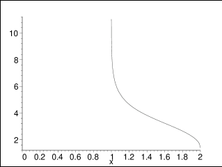
Figure 1: Deflection angle is a function of closest approach due to the C-field wormhole

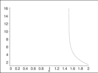
Figure 2: Schwarzschild deflection angle is a function of closest approach

4. Stability Analysis:

To study the stability, we match the interior C-field wormhole to the exterior Schwarzschild solution at a junction interface S, situated outside the event horizon, $a>r_{b}=2M$, one needs to use extrinsic curvature of S. The extrinsic curvature or second fundamental form is defined as $K_{ij}=n_{\mu;\nu}e^{\mu}_{(i)}e^{\nu}_{(j)}$, where $n^{\mu}$ is the unit normal 4 - vector to S and $e^{\mu}_{(i)}$ are the components of the holonomic basis vectors tangent to S. In general $K_{ij}$ is not continuous across S. The discontinuity in the extrinsic curvature is defined by $\kappa_{ij}=K_{ij}^{+}-K_{ij}^{-}$. Using the Darmois-Israel formalism, we write Lanczos equations for the surface stress energy tensors $S_{i}^{j}$ at the junction interface S as [26-32]

$$S_{i}^{j}=-\frac{1}{8\pi}[\kappa_{i}^{j}-\delta_{i}^{j}\kappa_{k}^{k}]$$ (26)

To analyze the dynamics of the wormhole, we permit the radius of the throat to become a function of time, $a\mapsto a(\tau)$.

The non trivial components of the extrinsic curvature are given by

$$K{{}_{\tau}^{\tau}}^{+}=\frac{\frac{M}{a^{2}}+\ddot{a}}{\sqrt{1-\frac{2M}{a}+\dot{a}^{2}}}$$ (27)

$$K{{}_{\tau}^{\tau}}^{-}=\frac{\ddot{a}-\frac{D\dot{a}}{a(a^{2}-D)}}{\sqrt{1-\frac{D}{a^{2}}+\dot{a}^{2}}}$$ (28)

and

$$K{{}_{\theta}^{\theta}}^{+}=\frac{1}{a}\sqrt{1-\frac{2M}{a}+\dot{a}^{2}}$$ (29)

$$K{{}_{\theta}^{\theta}}^{-}=\frac{1}{a}\sqrt{1-\frac{D}{a^{2}}+\dot{a}^{2}}$$ (30)

[ we have taken the wormhole space time metric (10) and Schwarzschild solution ]

The surface energy tensor may be written in terms of the surface energy density $\sigma$ and the surface pressure p as $S_{i}^{j}=dia(-\sigma,p,p)$.

Then from Lanczos equations, we get,

$$\sigma=-\frac{1}{4\pi a}[\sqrt{1-\frac{2M}{a}+\dot{a}^{2}}-\sqrt{1-\frac{D}{a^{2}}+\dot{a}^{2}}]$$ (31)

$$p=\frac{1}{8\pi a}[\frac{1-\frac{M}{a}+\dot{a}^{2}+a\ddot{a}}{\sqrt{1-\frac{2M}{a}+\dot{a}^{2}}}-\frac{1-\frac{D}{a^{2}}+\dot{a}^{2}+a\ddot{a}-\frac{aD\dot{a}^{2}}{(a^{3}-D)}}{\sqrt{1-\frac{D}{a^{2}}+\dot{a}^{2}}}]$$ (32)

Taking into account conservation identity ${S^{i}_{j}}_{|i}=[T_{\mu\nu}e^{\mu}_{(j)}n^{\nu}]_{-}^{+}$ and using ${S^{i}_{\tau}}_{|i}=-[\dot{\sigma}+\frac{2\dot{a}(\sigma+p)}{a}]$, one gets,

$$\sigma^{\prime}=-\frac{2(\sigma+p)}{a}+E$$ (33)

where

$$E=\frac{1}{4\pi a^{2}}[\frac{2D}{a(a^{2}-D)}]\sqrt{1-\frac{M}{a}+\dot{a}^{2}}$$ (34)

Rearranging equation (31), one can get the thin shell’s equation of motion i.e. $\dot{a}^{2}+V(a)=0$ with the potential is given by

$$V=1+A-B^{2}$$ (35)

where

$A=\frac{MD}{a^{2}C^{2}}$, $C=4\pi a^{2}\sigma$ and $B=2\pi a\sigma+\frac{M+\frac{D}{2a^{2}}}{4\pi a^{2}\sigma}$.

Linearizing around a static solution situated at $a_{0}$, one can get expand V(a) around $a_{0}$ to yield

$$V=V(a_{0})+V^{\prime}(a_{0})(a-a_{0})+\frac{1}{2}V^{\prime\prime}(a_{0})(a-a_{0})^{2}+0[(a-a_{0})^{3}]$$ (36)

One can verify that at the static solution, $a=a_{0}$, $V(a_{0})=0$ and $V^{\prime}(a_{0})=0$. From $V^{\prime}(a_{0})=0$, one can get an equlibrium relation as $\frac{dA}{da}\mid_{a_{0}}=2BB^{\prime}\mid_{a_{0}}$ [ see appendix for exact analytical form ].

Hence the potential equation reduces to

$$V=\frac{1}{2}V^{\prime\prime}(a_{0})(a-a_{0})^{2}+0[(a-a_{0})^{3}]$$ (37)

The solution is stable iff V(a) has a local minimum at $a_{0}$. Then the stability condition is $V^{\prime\prime}(a_{0})>0$ i.e. $A^{\prime\prime}\mid_{a_{0}}>2B^{\prime}{{}^{2}}\mid_{a_{0}}+2B\mid_{a_{0}}B^{\prime\prime}\mid_{a_{0}}$.

Hence one gets the following expression for stability condition of the C-field wormhole as

$$P>F+R$$ (38)

where P , F and R are given in the appendix.

Also, from (33), one can write,

$$\eta=-1+\frac{a}{2\sigma^{\prime}}[\frac{2}{a^{2}}(p+\sigma)+E^{\prime}-\sigma^{\prime\prime}]$$ (39)

where $\eta=\frac{p^{\prime}}{\sigma^{\prime}}$ and this parameter $\sqrt{\eta}$ is normally interpreted as the speed of sound [28]. Now we shall use $\eta$ as a parametrization of the stable equilibrium, to show the stability region graphically. To determine stability region of this solution we use, $b(a_{0})>2M$ i.e. when $\sigma<0$. Now we take $r_{0}=\sqrt{D}>2M,$ so that junction radius lies outside the event horizon i.e. $a_{0}>2M$. The junction radius lies in the following range $2M<a_{0}<\frac{D}{2M}$.

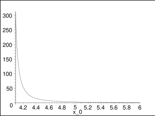
Figure 3: We define $x_{0}=\frac{a_{0}}{M}$ and choose $\frac{\sqrt{D}}{M}=3$. Here we plot $\eta_{|{(a=a_{0})}}$ $Vs.$ $x_{0}$ for the negative surface energy density. The stability region is given below the curve.

5. Conclusion:

Since the collection of exotic matter is undoubtedly an extremely hard task, many Scientists are given their attention to the alternative theories of gravity to obtain wormhole structure. In this work, we have considered C-field theory to obtain wormhole space time. Gravitational lensing seems to be an unique tool, on a theoretical ground, to detect exotic objects in the Universe, that, though not yet observed. We have discussed the gravitational lensing due to a C-field wormhole in the strong field limit. We have shown that the deflection angle of the C-field wormhole is very similar to the Schwarzschild solution. It has been shown that radius of the photon sphere is equal to the throat of the C-field wormhole. From the graph, one can see that the deflection angle $\alpha_{WH}$, diverges at the throat. Since we have matched the interior wormhole solution to the exterior Schwarzschild solution across a surface, at $r=a$, the deflection angle due to the both the cases should coincide. The graphs which have been depicted here support this. We have also analyzed the C-field wormhole solution by matching an interior solution to exterior Schwarzschild space time, at a junction surface. We have explained the stability of the spherically symmetric shell to linearized perturbation about static equilibrium solution. We have provided an exact analytical expression for stability of the C-field wormhole ( see equation (38)). For a lot of useful information, we have shown the stability region graphically. We have calculated the range where the junction radius would lie and have shown that stability region may be increased by increasing the wormhole throat.

Acknowledgments

F.R is thankful to Jadavpur University and DST , Government of India for providing financial support. MK has been partially supported by UGC, Government of India under MRP scheme. We are also grateful to the referee for his valuable comments.

Appendix

$\sigma_{0}=-\frac{1}{4\pi a_{0}}[\sqrt{1-\frac{2M}{a_{0}}}-\sqrt{1-\frac{D}{a_{0}^{2}}}]$

$\sigma^{\prime}_{0}=\frac{1}{4\pi a_{0}^{2}}[\frac{1-\frac{3M}{a_{0}}}{\sqrt{1-\frac{2M}{a_{0}}}}-\frac{1-\frac{2D}{a_{0}^{2}}}{\sqrt{1-\frac{D}{a_{0}^{2}}}}]$ $\sigma^{\prime\prime}_{0}=\frac{1}{4\pi a_{0}^{2}}[\frac{\frac{3M}{a_{0}^{2}}}{\sqrt{1-\frac{2M}{a_{0}}}}-\frac{M}{a_{0}^{2}}\frac{(1-\frac{3M}{a_{0}})}{(1-\frac{2M}{a_{0}})^{\frac{3}{2}}}-\frac{\frac{4D}{a_{0}^{3}}}{\sqrt{1-\frac{D}{a_{0}^{2}}}}+\frac{D}{a_{0}^{3}}\frac{(1-\frac{2D}{a_{0}^{2}})}{(1-\frac{D}{a_{0}^{2}})^{\frac{3}{2}}}]-\frac{1}{2\pi a_{0}^{3}}[\frac{(1-\frac{3M}{a_{0}})}{\sqrt{1-\frac{2M}{a_{0}}}}-\frac{(1-\frac{2D}{a_{0}^{2}})}{\sqrt{1-\frac{D}{a_{0}^{2}}}}]$

$[\frac{dA}{da}]_{a=a_{0}}=-\frac{MD}{8\pi^{2}\sigma_{0}^{2}a_{0}^{4}}-\frac{MD(2\sigma_{0}+a_{0}\sigma_{0}^{\prime})}{8\pi^{2}\sigma_{0}^{3}a_{0}^{7}}$

$[\frac{dB}{da}]_{a=a_{0}}=2\pi\sigma_{0}+2\pi a_{0}\sigma_{0}^{\prime}-\frac{D}{8\pi\sigma_{0}a_{0}^{5}}-(8\pi\sigma_{0}a_{0}+4\pi a_{0}^{2}\sigma_{0}^{\prime})\frac{(M+\frac{D}{2a_{0}})}{(4\pi\sigma_{0}a_{0}^{2})^{2}}$

$P=\frac{\frac{4MD}{a_{0}^{3}}}{(4\pi\sigma_{0}a_{0}^{2})^{2}}+\frac{8MD}{a_{0}^{2}}\frac{(8\pi a_{0}\sigma_{0}+4\pi\sigma_{0}^{\prime}a_{0}^{2})}{(4\pi\sigma_{0}a_{0}^{2})^{3}}-\frac{4MD}{a_{0}}\frac{(8\pi\sigma_{0}+16\pi a_{0}\sigma_{0}^{\prime}+4\pi a_{0}^{2}\sigma_{0}^{\prime\prime})}{(4\pi\sigma_{0}a_{0}^{2})^{3}}+\frac{12MD}{a_{0}}\frac{(8\pi\sigma_{0}a_{0}+4\pi a_{0}^{2}\sigma_{0}^{\prime})^{2}}{(4\pi\sigma_{0}a_{0}^{2})^{4}}$

$F=2[2\pi\sigma_{0}+2\pi a_{0}\sigma_{0}^{\prime}-\frac{D}{8\pi\sigma_{0}a_{0}^{5}}-(8\pi\sigma_{0}a_{0}+4\pi a_{0}^{2}\sigma_{0}^{\prime})\frac{(M+\frac{D}{2a_{0}})}{(4\pi\sigma_{0}a_{0}^{2})^{2}}]^{2}$

$R=2[2\pi a_{0}\sigma_{0}+\frac{M+\frac{D}{2a_{0}^{2}}}{4\pi a^{2}\sigma_{0}}][4\pi\sigma_{0}^{\prime}+2\pi a_{0}\sigma_{0}^{\prime\prime}+\frac{2D}{8\pi\sigma_{0}a_{0}^{5}}+\frac{D(8\pi\sigma_{0}a_{0}+4\pi a_{0}^{2}\sigma_{0}^{\prime})}{2a_{0}^{2}(4\pi\sigma_{0}a_{0}^{2})^{2}}-\frac{(M+\frac{D}{2a_{0}})}{(4\pi\sigma_{0}a_{0}^{2})^{2}}[8\pi\sigma_{0}+16\pi a_{0}\sigma_{0}^{\prime}+4\pi a_{0}^{2}\sigma_{0}^{\prime\prime}]+\frac{2(M+\frac{D}{2a_{0}})}{(4\pi\sigma_{0}a_{0}^{2})^{3}}[8\pi\sigma_{0}a_{0}+4\pi a_{0}^{2}\sigma_{0}^{\prime}]^{2}]$

The stability condition is $P>R+F$ i.e. if

$\frac{\frac{4MD}{a_{0}^{3}}}{(4\pi\sigma_{0}a_{0}^{2})^{2}}+\frac{8MD}{a_{0}^{2}}\frac{(8\pi a_{0}\sigma_{0}+4\pi\sigma_{0}^{\prime}a_{0}^{2})}{(4\pi\sigma_{0}a_{0}^{2})^{3}}-\frac{4MD}{a_{0}}\frac{(8\pi\sigma_{0}+16\pi a_{0}\sigma_{0}^{\prime}+4\pi a_{0}^{2}\sigma_{0}^{\prime\prime})}{(4\pi\sigma_{0}a_{0}^{2})^{3}}+\frac{12MD}{a_{0}}\frac{(8\pi\sigma_{0}a_{0}+4\pi a_{0}^{2}\sigma_{0}^{\prime})^{2}}{(4\pi\sigma_{0}a_{0}^{2})^{4}}>2[2\pi\sigma_{0}+2\pi a_{0}\sigma_{0}^{\prime}-\frac{D}{8\pi\sigma_{0}a_{0}^{5}}-(8\pi\sigma_{0}a_{0}+4\pi a_{0}^{2}\sigma_{0}^{\prime})\frac{(M+\frac{D}{2a_{0}})}{(4\pi\sigma_{0}a_{0}^{2})^{2}}]^{2}+2[2\pi a_{0}\sigma_{0}+\frac{M+\frac{D}{2a_{0}^{2}}}{4\pi a^{2}\sigma_{0}}][4\pi\sigma_{0}^{\prime}+2\pi a_{0}\sigma_{0}^{\prime\prime}+\frac{2D}{8\pi\sigma_{0}a_{0}^{5}}+\frac{D(8\pi\sigma_{0}a_{0}+4\pi a_{0}^{2}\sigma_{0}^{\prime})}{2a_{0}^{2}(4\pi\sigma_{0}a_{0}^{2})^{2}}-\frac{(M+\frac{D}{2a_{0}})}{(4\pi\sigma_{0}a_{0}^{2})^{2}}[8\pi\sigma_{0}+16\pi a_{0}\sigma_{0}^{\prime}+4\pi a_{0}^{2}\sigma_{0}^{\prime\prime}]+\frac{2(M+\frac{D}{2a_{0}})}{(4\pi\sigma_{0}a_{0}^{2})^{3}}[8\pi\sigma_{0}a_{0}+4\pi a_{0}^{2}\sigma_{0}^{\prime}]^{2}]$

The equilibrium relation is $\frac{dA}{da}\mid_{a_{0}}-2BB^{\prime}\mid_{a_{0}}=0$ i.e. if

$2(2\pi a_{0}\sigma_{0}+\frac{M+\frac{D}{2a_{0}^{2}}}{4\pi a_{0}^{2}\sigma_{0}})(2\pi\sigma_{0}+2\pi a_{0}\sigma_{0}^{\prime}-\frac{D}{8\pi\sigma_{0}a_{0}^{5}}-(8\pi\sigma_{0}a_{0}+4\pi a_{0}^{2}\sigma_{0}^{\prime})\frac{(M+\frac{D}{2a_{0}})}{(4\pi\sigma_{0}a_{0}^{2})^{2}})+\frac{MD}{8\pi^{2}\sigma_{0}^{2}a_{0}^{4}}+\frac{MD(2\sigma_{0}+a_{0}\sigma_{0}^{\prime})}{8\pi^{2}\sigma_{0}^{3}a_{0}^{7}}=0$

The values of $\sigma_{0}$, $\sigma^{\prime}_{0}$ and $\sigma^{\prime\prime}_{0}$ are given above.

References

• [1] M. Morris and K. Thorne , American J. Phys. 56, 39 (1988 )
• [2] F. Lobo, Phys.Rev.D71:084011,2005
• [3] S. Sushkov , Phys.Rev.D71:043520,2005
• [4] F. Lobo, Phys.Rev.D71:124022,2005
• [5] O. Zaslavskii arXiv: gr-qc / 0508057
• [6] F Rahaman, M Kalam, M Sarker and K Gayen, Phys.Lett.B633:161-163,2006( e-Print: gr-qc/0512075); F. Rahaman et al , gr-qc/0701032 ; F. Rahaman et al ,Gen.Rel.Grav.39:145-151,2007 ( e-Print: gr-qc/0611133 )
• [7] F. Lobo, Phys.Rev.D73:064028,2006
• [8] A Das and S Kar, Class.Quant.Grav.22:3045-3054,2005
• [9] M Mansouryar arXiv: gr-qc / 0511086
• [10] A Bhadra and K Sarkar , Mod.Phys.Lett.A20:1831-1844,2005
• [11] K K Nandi et al Phys. Rev. D 57, 823 (1997)
• [12] L Anchordoqui et al Phys. Rev. D 55, 5226 (1997)
• [13] A Agnese and M Camera Phys. Rev. D 51, 2011(1995)
• [14] F Rahaman, M Kalam and A Ghosh , Nuovo Cim.121B:303-307,2006 (e-Print: gr-qc/0605095)
• [15] E Eiroa and C Simeone Phys.Rev.D 70, 044008 (2004)
• [16] K K Nandi et al Phys. Rev. D 55, 2497 (1997)
• [17] Bronnikov K and Grinyok S , Grav.Cosmol.7:297-300,2001
• [18] Bronnikov K and Grinyok S, arXiv:gr-qc / 0205131
• [19] Bronnikov K , Phys.Rev.D67:064027,2003
• [20] Hoyle. F and Narlikar. J. V. Proc.Roy.Soc. A 290 (1966) 162; Narlikar. J and Padmanabhan.T, Phys.Rev.D 32, 1928 (1985); S.Chaterjee and A Banerjee, Gen.Rel.Grav.36:303-313,2004 ; F Rahaman et al , Astrophys.Space Sci.302, 171(2006); F Rahaman et al, Chin.J.Phys.43, 806(2005); F Rahaman et al, Int.J.Mod.Phys.A21:3727-3732,2006 ( e-Print: gr-qc/0601005 )
• [21] F Rahaman, B C Bhui and P Ghosh , Nuovo Cim.119B:1115-1119,2004 (e-Print: gr-qc/0512113)
• [22] K.S. Virbhadra, George F.R. Ellis, Phys.Rev.D62:084003,2000. [ASTRO-PH 9904193]; K.S. Virbhadra, D. Narasimha, S.M. Chitre, Astron.Astrophys.337:1-8,1998; K. S. Virbhadra, G. F. R. Ellis, Phys.Rev.D65:103004,2002; V Bozza , Phys.Rev.D66:103001,2002
• [23] Cramer J G et al , Phys.Rev.D51:3117-3120,1995
• [24] J S Tejeiro and E R Larrañagar, arXiv: gr-qc/ 0505054
• [25] Nandi K K , Y Zhang and A V Zakharov ,Phys.Rev.D74:024020,2006
• [26] W Israel Nuovo Cimento 44B , 1 (1966) ; erratum - ibid. 48B, 463 (1967)
• [27] M. Visser , Lorentzian Wormholes: From Einstien to Hawking , AIP Press (1995)
• [28] E Poisson and M Visser , Phys.Rev.D52:7318-7321,1995
• [29] F Lobo, Class.Quant.Grav.21:4811-4832,2004; F Lobo and P Crawford, Class.Quant.Grav.22:4869-4886,2005
• [30] E Eiroa and E Romero , Gen.Rel.Grav.36:651-659,2004
• [31] M Ishak and K Lake , Phys.Rev.D65:044011,2002
• [32] F.Rahaman et al, Gen.Rel.Grav.38, 1687 (2006) ( e-Print: gr-qc/0607061 ); F.Rahaman et al, gr-qc/0611134 ; F.Rahaman et al, gr-qc/0703143
• [33] A Taub J Math. Phys. 21, 1423 (1980)
• [34] J Lemos, F Lobo and S Oliveira , Phys.Rev.D68:064004,2003
• [35] H G Ellis J. Math. Phys. 14, 104 (1973)