Small Chvátal Rank

Abstract.

We propose a variant of the Chvátal-Gomory procedure that will produce a sufficient set of facet normals for the integer hulls of all polyhedra $\{{\bf{x}}\,:\,A{\bf{x}}\leq{\bf{b}}\}$ as ${\bf{b}}$ varies. The number of steps needed is called the small Chvátal rank (SCR) of $A$. We characterize matrices for which SCR is zero via the notion of supernormality which generalizes unimodularity. SCR is studied in the context of the stable set problem in a graph, and we show that many of the well-known facet normals of the stable set polytope appear in at most two rounds of our procedure. Our results reveal a uniform hypercyclic structure behind the normals of many complicated facet inequalities in the literature for the stable set polytope. Lower bounds for SCR are derived both in general and for polytopes in the unit cube.

1. Introduction

The study of integer hulls of rational polyhedra is a fundamental area of research in integer programming. For a matrix $A\in\mathbb{Z}^{m\times n}$ and a vector ${\bf{b}}\in\mathbb{Z}^{m}$, consider the polyhedron

$$Q_{\bf{b}}:=\{{\bf x}\in\mathbb{R}^{n}\,:\,A{\bf x}\leq{\bf{b}}\}$$

and its integer hull

$$Q_{\bf{b}}^{I}:=\textup{convex hull}(Q_{\bf{b}}\cap\mathbb{Z}^{n}).$$

The Chvátal-Gomory procedure is an algorithm for computing $Q_{\bf{b}}^{I}$ from $Q_{\bf{b}}$. This method involves iteratively adding rounds of cutting planes to $Q_{\bf{b}}$ until $Q_{\bf{b}}^{I}$ is obtained. The Chvátal rank of $A{\bf{x}}\leq{\bf{b}}$ is the minimum number of rounds of cuts needed in the Chvátal-Gomory procedure to obtain $Q_{\bf{b}}^{I}$, and the Chvátal rank of $A$ is the maximum of the Chvátal ranks of $A{\bf{x}}\leq{\bf{b}}$ as ${\bf{b}}$ varies in $\mathbb{Z}^{m}$.

In this paper we fix a matrix $A\in\mathbb{Z}^{m\times n}$ of rank $n$ and look at the more basic problem of finding just the normals of a sufficient set of inequalities that will cut out all integer hulls $Q_{\bf{b}}^{I}$ as ${\bf{b}}$ varies in $\mathbb{Z}^{m}$. Given $A$, it is known that there exists a matrix $M$ such that for each ${\bf{b}}$, $Q_{\bf{b}}^{I}=\{{\bf{x}}\in\mathbb{R}^{n}\,:\,M{\bf{x}}\leq{\bf{d}}\}$ for some ${\bf{d}}$ [16, Theorem 17.4]. The set of rows of $M$ can be chosen to be

$$\{{\bf{m}}\in\mathbb{Z}^{n}\,:\,{\bf{m}}={\bf{y}}A,\,{\bf{y}}\geq{\bf 0},\,||{\bf{m}}||_{\infty}\leq n^{2n}\Delta^{n}\}$$

where $\Delta$ is the maximum absolute value of a minor of $A$. In practice, $M$ could be much smaller. For instance if $A$ is the $4\times 2$ matrix with rows $(1,2)$, $(-2,-3)$, $(1,0)$ and $(0,1)$, it suffices to augment $A$ with the rows $(1,1),(0,-1),(-1,-2),(-1,-1)$, while $n^{2n}\Delta^{n}=144$.

In Section 2 we introduce a vector version of the Chvátal-Gomory procedure called iterated basis normalization (IBN) that constructs a sufficient $M$ from the matrix $A$. The small Chvátal rank (SCR) of $A$ is the number of rounds of IBN necessary to generate this $M$. A similar definition can be made when ${\bf{b}}$ is fixed. The SCR of $A$ (respectively of $A{\bf x}\leq{\bf{b}}$) is at most its Chvátal rank even though IBN may not terminate when $n\geq 3$. We show that in every dimension, there are systems $A{\bf{x}}\leq{\bf{b}}$ for which SCR is two while the Chvátal rank is arbitrarily high.

In Section 3 we completely characterize matrices for which SCR is zero. This requires the notion of supernormality introduced in [11] which generalizes the familiar notion of unimodularity. We produce a family of matrices of increasing dimension for which SCR is zero but Chvátal rank is not zero.

In Section 4 we apply the theory of SCR to $\textup{FRAC}(G)$, the fractional stable set polytope of a graph $G$. We determine the structure of the vectors produced by IBN in rounds one and two. As a consequence we see that the normals of many of the well-known facet inequalities of the stable set polytope, $\textup{STAB}(G)$, appear within two rounds of IBN. It is a long-standing open problem to describe $\textup{STAB}(G)$ when $G$ is a claw-free graph. We show that many of the complicated facet normals of $\textup{STAB}(G)$ when $G$ is claw-free appear in two rounds of IBN which reveals a uniform hypercyclic structure in these ad hoc examples.

Section 5 contains lower bounds for SCR which contrast with the results in the earlier sections. We show that if $n\geq 3$, SCR may grow exponentially in the bit size of the matrix $A$, asymptotically just as fast as Chvátal rank. For polytopes in the unit cube $[0,1]^{n}$, SCR can be at least $n/2$. We also exhibit a lower bound that depends on $n$ for $\textup{SCR}(\textup{FRAC}(G))$ as $G$ varies over all graphs with $n$ vertices. A brief discussion of possible upper bounds and computational evidence supporting our guesses are also provided.

The SCR of $A{\bf{x}}\leq{\bf{b}}$ or $A$ offers a coarser measure than Chvátal rank of the complexity of the integer programs associated to them. The goal here is to determine how quickly the facet normals of an integer hull are produced from the normals of the rational polyhedron, ignoring the right-hand-sides of the facet inequalities. Our main message is that, in many cases, facet normals are produced surprisingly fast by the Chvátal-Gomory procedure but the right-hand-side can take a long time to be computed, which makes Chvátal rank high. The coarseness of SCR can be a powerful organizational tool that can reveal the unifying structure behind seemingly ad hoc facet normals of a class of examples. An illustration of this philosophy can be found in Example 4.10 where we show that many difficult facet normals that have been found for the stable set polytope of a claw-free graph are produced within two rounds of IBN. While the Chvátal-Gomory procedure carries along both the number theoretic and geometric parts of an integer hull computation, SCR focuses on the number theory alone, often revealing interesting structural facts that are difficult to see through the fine Chvátal-Gomory lens.

2. Main Definitions.

Fix a matrix $A\in\mathbb{Z}^{m\times n}$ of rank $n$ and let $\mathcal{A}=\{{\bf{a}}_{1},\ldots,{\bf{a}}_{m}\}$  be the vector configuration in $\mathbb{Z}^{n}$ consisting of the rows of $A$. We assume that each row of $A$ is primitive (i.e., the gcd of its components is one). For each ${\bf{b}}\in\mathbb{Z}^{m}$, consider the rational polyhedron $Q_{\bf{b}}:=\{{\bf{x}}\in\mathbb{R}^{n}\,:\,A{\bf{x}}\leq{\bf{b}}\}$ and its integer hull $Q_{\bf{b}}^{I}:=\textup{conv}(Q_{\bf{b}}\cap\mathbb{Z}^{n})$ where conv denotes convex hull. Since $\textup{rank}(A)=n$, every minimal face of $Q_{\bf{b}}$, and $Q_{\bf{b}}^{I}$ (if non-empty), is a vertex. A Hilbert basis of a rational polyhedral cone $K\subseteq\mathbb{R}^{n}$ is a set $\{{\bf{h}}_{1},\ldots,{\bf{h}}_{t}\}\subset K\cap\mathbb{Z}^{n}$ such that if ${\bf{k}}\in K\cap\mathbb{Z}^{n}$ then ${\bf{k}}=\sum_{i=1}^{t}n_{i}{\bf{h}}_{i}$ where $n_{i}\in\mathbb{N}$. If $K$ is pointed then it has a unique minimal Hilbert basis. Write $\textup{Hilb}(K)$ (respectively, $\textup{Hilb}(\mathcal{A})$) for a minimal Hilbert basis of $K$ (respectively, $\textup{cone}(\mathcal{A})$).

The Chvátal-Gomory procedure [6], [16, §23] for computing $Q_{\bf{b}}^{I}$ works as follows. For each vertex ${\bf{v}}$ of $Q_{{\bf{b}}}$, set $\mathcal{A}_{{\bf{v}}}:=\{{\bf{a}}_{i}\in\mathcal{A}:{\bf{a}}_{i}\cdot{\bf{v}}=b_{i}\}$ and define $Q_{{\bf{b}}}^{(1)}$ to be the polyhedron cut out by the inequalities ${\bf{h}}\cdot{\bf{x}}\leq\lfloor{\bf{h}}\cdot{\bf{v}}\rfloor$ for every vertex ${\bf{v}}$ of $Q_{{\bf{b}}}$ and every vector ${\bf{h}}\in\textup{Hilb}(\mathcal{A}_{\bf{v}})$. Then $Q_{{\bf{b}}}^{I}\subseteq Q_{{\bf{b}}}^{(1)}\subseteq Q_{{\bf{b}}}$. For $i\geq 2$, define $Q_{{\bf{b}}}^{(i)}:=(Q_{{\bf{b}}}^{(i-1)})^{(1)}$. For a positive integer $k$, $Q_{\bf{b}}^{(k)}$ is called the $k$-th Chvátal closure of $Q_{\bf{b}}$. The Chvátal rank of $A{\bf{x}}\leq{\bf{b}}$ (equivalently, $Q_{\bf{b}}$) is the smallest number $t$ such that $Q_{{\bf{b}}}^{(t)}=Q_{\bf{b}}^{I}$. This rank only depends on $Q_{\bf{b}}$ and not the inequality system defining it. The Chvátal rank of $A$ is the maximum over all ${\bf{b}}\in\mathbb{Z}^{m}$ of the Chvátal ranks of $A{\bf{x}}\leq{\bf{b}}$. The Chvátal-Gomory procedure and the Chvátal ranks are all finite [16, Chapter 23].

To study just the facet normals of the integer hulls $Q_{\bf{b}}^{I}$ for every ${\bf{b}}$, we modify the Chvátal-Gomory procedure as follows. An $n$-subset $\tau\subseteq[m]:=\{1,2,\ldots,m\}$ is called a basis if the submatrix $A_{\tau}$, consisting of the rows of $A$ indexed by $\tau$, is non-singular. Let $\mathcal{A}_{\tau}$ be the set of rows of $A_{\tau}$. We call $\textup{cone}(\mathcal{A}_{\tau})$ a basis cone since $\mathcal{A}_{\tau}$ is a basis of $\mathbb{R}^{n}$. The set $\mathcal{A}$ contains at least one basis cone since $\textup{rank}(A)=n$.

Observation 2.1.

Suppose $\sigma\subseteq[m]$ such that $\mathcal{A}_{\sigma}$ linearly spans $\mathbb{R}^{n}$. Then the union of the minimal Hilbert bases of the basis cones $\textup{cone}(\mathcal{A}_{\tau})$, as $\tau$ varies over the bases contained in $\sigma$, is a Hilbert basis for $\textup{cone}(\mathcal{A}_{\sigma})$.

Algorithm 2.2.

Iterated Basis Normalization (IBN)
Input: $A\in\mathbb{Z}^{m\times n}$ satisfying the assumptions above.

1. Set $\mathcal{A}^{(0)}:=\mathcal{A}$.

2. For $k\geq 1$, let $\mathcal{A}^{(k)}$ be the union of all the (unique) minimal Hilbert bases of all basis cones in $\mathcal{A}^{(k-1)}$.

3. If $\mathcal{A}^{(k)}=\mathcal{A}^{(k-1)}$, then stop. Otherwise repeat.

Remark 2.3.

Since each vector in $\mathcal{A}$ is primitive, $\mathcal{A}\subseteq\mathcal{A}^{(1)}.$ Every vector created during IBN is also primitive and so $\mathcal{A}\subseteq\mathcal{A}^{(1)}\subseteq\mathcal{A}^{(2)}\subseteq\ldots$.

Lemma 2.4.

If all elements of $\mathcal{A}$ are non-negative except for the negative unit vectors $-{\bf{e}}_{i},i\in[n]$, then for each non-negative integer $k$, all vectors in $\mathcal{A}^{(k)}$ besides the original $-{\bf{e}}_{i}$’s are also non-negative.

Proof:   The claim holds for $k=0$, and suppose it holds up to $k-1$. When IBN constructs $\mathcal{A}^{(k)}$ from $\mathcal{A}^{(k-1)}$, for each $i\in[n]$, the only vector available with negative $i$-th coordinate is $-{\bf{e}}_{i}$ but since its multiplier lies in $[0,1)$, the $i$th coordinate of the resulting Hilbert basis elements cannot be negative. $\square$

Let $A^{(k)}$ denote a matrix whose rows are the elements of $\mathcal{A}^{(k)}$ with the rows in $\mathcal{A}^{(k)}\setminus\mathcal{A}^{(k-1)}$ appended at the bottom of $A^{(k-1)}$.

Definition 2.5.

1. The small Chvátal rank (SCR) of the system of inequalities $A{\bf{x}}\leq{\bf{b}}$ defining $Q_{\bf{b}}$ is the smallest number $k$ such that there is an integer vector ${\bf{b}}^{\prime}$ satisfying

   $$Q_{\bf{b}}^{I}\,=\,\{{\bf{x}}\in\mathbb{R}^{n}\,:\,A^{(k)}{\bf{x}}\leq{\bf{b}}^{\prime}\}.$$

2. The SCR of a matrix $A$ is the supremum of the SCRs of all systems of the form $A{\bf{x}}\leq{\bf{b}}$ as ${\bf{b}}$ varies in $\mathbb{Z}^{m}$.

Proposition 2.6.

For any ${\bf{b}}\in\mathbb{Z}^{m}$, the SCR of $A{\bf{x}}\leq{\bf{b}}$ is at most the Chvátal rank of the same system, and the SCR of $A\in\mathbb{Z}^{m\times n}$ is at most the Chvátal rank of $A$. In particular, the SCR is always finite.

Proof:   If ${\bf{v}}$ is a vertex of some intermediate polyhedron $Q_{\bf{b}}^{(i)}=\{{\bf{x}}\,:\,U{\bf{x}}\leq{\bf{u}}\}$ in the Chvátal-Gomory procedure, then $\mathcal{U}_{\bf{v}}$ linearly spans $\mathbb{R}^{n}$. By Observation 2.1 and induction, a Hilbert basis of $\mathcal{U}_{\bf{v}}$ is contained in $\mathcal{A}^{(i+1)}$ and therefore, $\mathcal{A}^{(i+1)}$ contains the normals of an inequality system describing $Q_{\bf{b}}^{(i)}$. In particular, if the Chvátal rank of $A{\bf{x}}\leq{\bf{b}}$ is $t$, then the normals of an inequality system describing $Q_{{\bf{b}}}^{I}$ are in $\mathcal{A}^{(t)}$. $\square$

Lemma 2.7.

When $n=2$, $\mathcal{A}^{(2)}=\mathcal{A}^{(1)}$, and IBN terminates in one round.

Proof:   Pick ${\bf{r}},{\bf{s}}\in\mathcal{A}^{(1)}\subset\mathbb{Z}^{2}$ such that $\textup{cone}({\bf{r}},{\bf{s}})$ is a basis cone. Let

$${\bf{t}}_{1}:={\bf{r}},{\bf{t}}_{2},\ldots,{\bf{t}}_{k-1},{\bf{t}}_{k}:={\bf{s}}$$

be the elements of $\mathcal{A}^{(1)}$ in $\textup{cone}({\bf{r}},{\bf{s}})$ in cyclic order from ${\bf{r}}$ to ${\bf{s}}$. Then for each $i\in\{1,\ldots,k-1\}$, $\textup{cone}({\bf{t}}_{i},{\bf{t}}_{i+1})$ is unimodular. (This is an artifact of $\mathbb{R}^{2}$. See [15, Corollary 3.11] for a proof.) Hence a Hilbert basis of $\textup{cone}({\bf{r}},{\bf{s}})$ is contained in $\{{\bf{t}}_{1},\ldots,{\bf{t}}_{k}\}$, and $A^{(2)}=\mathcal{A}^{(1)}$. $\square$

Corollary 2.8.

If $A\in\mathbb{Z}^{m\times 2}$, then the SCR of $A$ is at most one.

Example 2.9.

In contrast, Chvátal rank can be arbitrarily large even for $A\in\mathbb{Z}^{3\times 2}$. Fix $j\geq 1$ and consider the system $A{\bf{x}}\leq{\bf{b}}$ where

$$A=\left(\begin{array}[]{rr}-1&0\\ 1&2j\\ 1&-2j\end{array}\right)\,\textup{and}\;{\bf{b}}=(0,2j,0)^{t}.$$

The polyhedron $Q_{\bf{b}}$ is a triangle in $\mathbb{R}^{2}$ with vertices $(0,0)$, $(0,1)$ and $(j,1/2)$, and $Q_{\bf{b}}^{I}$ is the line segment from $(0,0)$ to $(0,1)$. It is noted in [16, §23.3] that the Chvátal rank of $A{\bf{x}}\leq{\bf{b}}$ is at least $j$.

Fix $n\geq 2$ and $m\geq n+1$. By taking the product of $Q_{\bf{b}}$ from above with the $(n-2)$-dimensional positive orthant and then adjoining $m-n-1$ redundant inequalities, we can produce $A^{\prime}{\bf{x}}\leq{\bf{b}}^{\prime}$, $A^{\prime}\in\mathbb{Z}^{m\times n}$ with the same property that SCR is one but Chvátal rank is arbitrarily large.

Unlike for $n\leq 2$, IBN need not terminate when $n>2$.

Example 2.10.

Take $\mathcal{A}=\{(0,3,1),(1,1,1),(2,5,5),(1,4,3)\}$. For each positive integer $k$, set

$${\bf{u}}_{k}:=(k,2k+2,2k+1)\,\,\,\textup{and}\,\,\,{\bf{v}}_{k}:=(k,2k+1,2k).$$

Note that ${\bf{u}}_{1}=(1,4,3)$ is a row of $A$. To show that IBN does not terminate on $\mathcal{A}$, one can check the following two assertions. We omit the details.

1. For each $k\geq 1$, ${\bf{v}}_{k}\in\textup{Hilb}(\{(0,3,1),(1,1,1),{\bf{u}}_{k}\})$.

2. For each $k\geq 1$, ${\bf{u}}_{k+1}\in\textup{Hilb}(\{(0,3,1),(2,5,5),{\bf{v}}_{k}\})$.

A second such example appears in [11].

Despite this example, the SCR of any matrix or system of inequalities is finite, and we will illustrate ways to bound it in many instances.

Definition 2.11.

For a positive integer $k$, the $k$-th small Chvátal closure of $A{\bf{x}}\leq{\bf{b}}$ is the set $S_{A,{\bf{b}}}^{(k)}:=\{{\bf{x}}\in\mathbb{R}^{n}\,:\,{\bf{a}}\cdot{\bf{x}}\leq m_{\bf{a}},\,\,{\bf{a}}\in\mathcal{A}^{(k)}\}$ where $m_{\bf{a}}:=\textup{max}\{{\bf{a}}\cdot{\bf{x}}\,:\,A{\bf{x}}\leq{\bf{b}},\,\,{\bf{x}}\in\mathbb{Z}^{n}\}$.

This is a definition for inequality systems: if $P=\{{\bf{x}}\in\mathbb{R}^{n}\,:\,A{\bf{x}}\leq{\bf{b}}\}=\{{\bf{x}}\in\mathbb{R}^{n}\,:\,A^{\prime}{\bf{x}}\leq{\bf{b}}^{\prime}\}$, then for a given $k$, $S_{A,{\bf{b}}}^{(k)}$ may not equal $S_{A^{\prime},{\bf{b}}^{\prime}}^{(k)}$. However, for a fixed $A{\bf{x}}\leq{\bf{b}}$, $S_{A,{\bf{b}}}^{(k)}\subseteq Q_{\bf{b}}^{(k)}$ for each non-negative integer $k$.

Lemma 2.12.

The SCR of $A{\bf{x}}\leq{\bf{b}}$ is the smallest integer $k$ such that $Q_{\bf{b}}^{I}=S_{A,{\bf{b}}}^{(k)}$.

Proof:   If $\textup{SCR}(A{\bf{x}}\leq{\bf{b}})=k$, then $Q_{\bf{b}}^{I}=\{{\bf{x}}\in\mathbb{R}^{n}\,:\,{\bf{a}}\cdot{\bf{x}}\leq b_{\bf{a}},\,\,{\bf{a}}\in\mathcal{A}^{(k)}\}$ for some scalars $b_{\bf{a}}$. However, $b_{\bf{a}}\geq m_{\bf{a}}$ for each ${\bf{a}}\in\mathcal{A}^{(k)}$, so $S_{A,{\bf{b}}}^{(k)}\subseteq\{{\bf{x}}\in\mathbb{R}^{n}\,:\,A{\bf{x}}\leq{\bf{b}}\}^{I}$, and hence they are equal. On the other hand, $S_{A,{\bf{b}}}^{(k-1)}\neq Q_{\bf{b}}^{I}$ since otherwise $\textup{SCR}(A{\bf{x}}\leq{\bf{b}})$ would be less than $k$. $\square$

3. Matrices with small Chvátal rank zero

We begin our study of SCR by characterizing the matrices $A$ for which SCR is zero. These are precisely the $A$’s with the property that for each ${\bf{b}}\in\mathbb{Z}^{m}$, there is a ${\bf{b}}^{\prime}\in\mathbb{Z}^{m}$ such that $Q_{\bf{b}}^{I}=\{{\bf{x}}\in\mathbb{R}^{n}\,:\,A{\bf{x}}\leq{\bf{b}}^{\prime}\}$. Our characterization offers a generalization of the familiar notion of unimodularity.

Definition 3.1.

A vector configuration $\mathcal{A}$ in $\mathbb{Z}^{n}$ is unimodular if for every subset $\mathcal{A}^{\prime}$ of $\mathcal{A}$, $\mathcal{A}^{\prime}$ is a Hilbert basis for $\textup{cone}(\mathcal{A}^{\prime})$.

Definition 3.2.

[16, Theorem 22.5] A system of linear inequalities $A{\bf{x}}\leq{\bf{b}}$ is totally dual integral (TDI) if the set $\mathcal{A}_{F}:=\{{\bf{a}}_{i}\in\mathcal{A}\,:\,{\bf{a}}_{i}{\bf{x}}=b_{i}\,\,\forall\,\,{\bf{x}}\in F\}$ is a Hilbert basis of the cone it generates for every face $F$ of the polyhedron $Q_{{\bf{b}}}=\{{\bf{x}}\,:\,A{\bf{x}}\leq{\bf{b}}\}$.

The following characterizations of matrices with Chvátal rank zero are well-known, while characterizations of higher Chvátal rank are unknown.

Theorem 3.3.

[16] Let $\mathcal{A}=\{{\bf{a}}_{1},\ldots,{\bf{a}}_{m}\}\subset\mathbb{Z}^{n}$ be such that the matrix $A$ whose rows are ${\bf{a}}_{1},\ldots,{\bf{a}}_{m}$ has rank $n$. Then the following are equivalent:

1. $\mathcal{A}$ is unimodular.

2. Every basis in $\mathcal{A}$ is a basis of $\mathbb{Z}^{n}$ as a lattice.

3. Every (regular) triangulation of $\mathcal{A}$ is unimodular.

4. For all ${\bf{b}}\in\mathbb{Z}^{m}$, the inequality system $A{\bf{x}}\leq{\bf{b}}$ is TDI.

5. For all ${\bf{b}}\in\mathbb{Z}^{m}$, the polyhedron $Q_{{\bf{b}}}=\{{\bf{x}}\in\mathbb{R}^{n}\,:\,A{\bf{x}}\leq{\bf{b}}\}$ is integral.

6. The Chvátal rank of $A$ is zero.

Theorem 3.5 will provide a complete analogue to Theorem 3.3 when SCR replaces Chvátal rank. A vector configuration $\mathcal{A}$ in $\mathbb{Z}^{n}$ is normal if it is a Hilbert basis for $\textup{cone}(\mathcal{A})$.

Definition 3.4.

[11] A configuration $\mathcal{A}$ is supernormal if for every subset $\mathcal{A}^{\prime}$ of $\mathcal{A}$, $\mathcal{A}\cap\textup{cone}(\mathcal{A}^{\prime})$ is a Hilbert basis of $\textup{cone}(\mathcal{A}^{\prime})$.

Following [11], we say that a system $A{\bf{x}}\leq{\bf{b}}$ is tight if for each $i=1,\ldots,m$, the hyperplane ${\bf{a}}_{i}{\bf{x}}=b_{i}$ contains an integer point in $Q_{\bf{b}}$ and hence supports $Q_{{\bf{b}}}^{I}$. When the inequality system is clear, we simply say that the polyhedron $Q_{{\bf{b}}}=\{{\bf{x}}\,:\,A{\bf{x}}\leq{\bf{b}}\}$ is tight. If $Q_{\bf{b}}^{I}$ is nonempty, recall that

$$m_{{\bf{a}}_{i}}:=\textup{max}\{{\bf{a}}_{i}\cdot{\bf{x}}\,:\,{\bf{x}}\in Q_{{\bf{b}}}^{I}\}\,\,\,\textup{for}\,\,\,i=1,\ldots,m$$

and set $\beta:=(m_{{\bf{a}}_{i}})\in\mathbb{Z}^{m}$. Then $Q_{\bf{b}}\supseteq Q_{\beta}\supseteq Q_{\bf{b}}^{I}$ and $Q_{\beta}$ is tight.

Theorem 3.5.

Let $\mathcal{A}=\{{\bf{a}}_{1},\ldots,{\bf{a}}_{m}\}\subset\mathbb{Z}^{n}$ be a configuration of primitive vectors such that the matrix $A$ whose rows are ${\bf{a}}_{1},\ldots,{\bf{a}}_{m}$ has rank $n$. Then the following are equivalent.

1. $\mathcal{A}$ is supernormal.

2. Every basis $\mathcal{A}^{\prime}$ in $\mathcal{A}$ has the property that $\mathcal{A}\cap\textup{cone}(\mathcal{A}^{\prime})$ is a Hilbert basis of $\textup{cone}(\mathcal{A}^{\prime})$, or equivalently, $\mathcal{A}=\mathcal{A}^{(1)}$.

3. Every (regular) triangulation of $\mathcal{A}$ that uses all the vectors is unimodular.

4. For all ${\bf{b}}\in\mathbb{Z}^{m}$, $A{\bf{x}}\leq{\bf{b}}$ is TDI whenever $Q_{{\bf{b}}}$ is tight.

5. For all ${\bf{b}}\in\mathbb{Z}^{m}$, the polyhedron $Q_{{\bf{b}}}$ is integral whenever $Q_{\bf{b}}$ is tight.

6. The SCR of $A$ is zero.

The equivalence of (1), (3), and (4) is shown in [11, Proposition 3.1 and Theorem 3.6]. Our contribution is the remaining set of equivalences.

Proof:  

[(1) $\Rightarrow$ (2)]: This is immediate from the definition of supernormality.

[(2) $\Rightarrow$ (3)]: Let $T$ be a triangulation of $\mathcal{A}$ using all of the vectors and $\sigma$ index a maximal simplex of $T$. Then the sub-configuration $\mathcal{A}_{\sigma}$ is a basis of $\mathcal{A}$ and by (2), $\mathcal{A}$ contains $\textup{Hilb}(\mathcal{A}_{\sigma})$. But since every vector in $\mathcal{A}$ is used in the triangulation $T$, none can lie inside or on the boundary of $\textup{cone}(\mathcal{A}_{\sigma})$ except those in $\mathcal{A}_{\sigma}$ itself. Thus $\mathcal{A}_{\sigma}$ is the Hilbert basis of its own cone. This implies that $\mathcal{A}_{\sigma}$ is a lattice basis, so $\sigma$ is a unimodular simplex. Since $\sigma$ was arbitrary, $T$ is a unimodular triangulation.

[(4) $\Rightarrow$ (5)]: This follows from [16, Corollary 22.1c], which says that for a ${\bf{b}}\in\mathbb{Z}^{m}$, if $A{\bf{x}}\leq{\bf{b}}$ is TDI, then $Q_{\bf{b}}$ is integral.

[(5) $\Leftrightarrow$ (6)]: Suppose $Q_{\bf{b}}$ with ${\bf{b}}\in\mathbb{Z}^{m}$ is integral whenever it is tight. Then for ${\bf{b}}\in\mathbb{Z}^{m}$ with $Q_{{\bf{b}}}^{I}\neq\emptyset$, $Q_{\beta}$ is integral since it is tight. But $Q_{{\bf{b}}}^{I}\subseteq Q_{\beta}\subseteq Q_{{\bf{b}}}$ which implies that $Q_{\beta}=Q_{{\bf{b}}}^{I}$ and the SCR of $A$ is zero.

Suppose the SCR of $A$ is zero and some $Q_{{\bf{b}}}$ is tight. Then no new facet normals are needed for $Q_{{\bf{b}}}^{I}$, so $Q_{\bf{b}}^{I}=Q_{\beta}\subseteq Q_{{\bf{b}}}$. Since for $i=1,\ldots,m$, ${\bf{a}}_{i}\cdot{\bf{x}}=b_{i}$ and ${\bf{a}}_{i}\cdot{\bf{x}}=m_{{\bf{a}}_{i}}$ both support $Q_{{\bf{b}}}^{I}$, $\beta={\bf{b}}$. Thus $Q_{\bf{b}}=Q_{\beta}$ is integral.

[(6) $\Rightarrow$ (3)]: Suppose there exists a non-unimodular (regular) triangulation $T$ of $\mathcal{A}$ that uses all the vectors in $\mathcal{A}$. Let $\mathcal{A}^{\prime}$ be a basis in $\mathcal{A}$ whose elements form a non-unimodular facet in $T$ and let $A^{\prime}$ be the non-singular square matrix whose rows are the elements of $\mathcal{A}^{\prime}$. Then there exists a ${\bf{b}}^{\prime}\in\mathbb{Z}^{n}$ such that $\{{\bf{x}}\in\mathbb{R}^{n}\,:\,A^{\prime}{\bf{x}}\leq{\bf{b}}^{\prime}\}$ is tight and its unique vertex is not integral. Since no element of $\mathcal{A}\backslash\mathcal{A}^{\prime}$ lies in $\textup{cone}(\mathcal{A}^{\prime})$, by choosing very large right-hand-sides for the elements in $\mathcal{A}\backslash\mathcal{A}^{\prime}$, one gets a $Q_{\bf{b}}$ in which the fractional vertex of $\{{\bf{x}}\in\mathbb{R}^{n}\,:\,A^{\prime}{\bf{x}}\leq{\bf{b}}^{\prime}\}$ and its neighborhood survive. Further, ${\bf{b}}$ can be chosen so that $Q_{\bf{b}}$ is tight. Therefore, the SCR of $A$ is not zero. $\square$

Example 3.6.

If the rows of $A$ are not primitive then supernormality is not necessary for the SCR of $A$ to be zero. Take $\mathcal{A}=\{(2,0),(0,2)\}$. Then for each ${\bf{b}}\in\mathbb{Z}^{2}$, $Q_{{\bf{b}}}=\{(x_{1},x_{2})\in\mathbb{R}^{2}\,:\,x_{1}\leq\frac{b_{1}}{2},\,\,x_{2}\leq\frac{b_{2}}{2}\}$. Hence $Q_{{\bf{b}}}$ is tight if and only if both $b_{1}$ and $b_{2}$ are even, in which case it has the unique integer vertex $(\frac{b_{1}}{2},\frac{b_{2}}{2})$. Therefore all tight $Q_{{\bf{b}}}$’s are integral but $A$ is not supernormal. It is easy to see that the SCR of $A$ is zero.

Remark 3.7.

If the dimension $n$ is fixed, then it is possible to determine whether $\mathcal{A}$ is supernormal (and hence whether SCR is zero) in polynomial time. The number of basis cones is at most $m\choose n$, so it suffices to check whether $\mathcal{A}\cap\textup{cone}(\mathcal{A}^{\prime})$ is normal for each basis $\mathcal{A}^{\prime}$ in $\mathcal{A}$. Barvinok and Woods [3, Theorem 7.1] show that in fixed dimension, a rational generating function for the Hilbert basis of each cone can be computed in polynomial time. We then subtract the polynomial $\sum_{{\bf{a}}\in\textup{cone}(\mathcal{A}^{\prime})\cap\mathcal{A}}{\bf{x}}^{\bf{a}}$ from this rational function, square the difference, and evaluate at ${\bf{x}}=(1,\ldots,1)$. This can also be done in polynomial time  [3, Theorem 2.6] and the result is zero if and only if $\mathcal{A}\cap\textup{cone}(\mathcal{A}^{\prime})$ is normal.

Problem 3.8.

Can one recognize the supernormality of $A$ in polynomial time analogous to Seymour’s result for unimodularity [19], [16, Chapter 20]?

We close this section with a family of matrices for which Chvátal rank is not zero while SCR is. The existence of such families was a question in [11].

Proposition 3.9.

There exist configurations in arbitrary dimension which are supernormal but not unimodular.

Proof:   Let $k$ be a positive integer and $\mathcal{A}$ be the rows of the $(2k+1)\times(2k+1)$ matrix

$$A=\left(\begin{array}[]{rrrrrr}1&1&0&\ldots&0&0\\ 0&1&1&\ldots&0&0\\ &&&\vdots&&\\ 0&0&0&\ldots&1&1\\ 1&0&0&\ldots&0&1\end{array}\right).$$

That is, $A$ is the edge-vertex incidence matrix of an odd circuit. The determinant of $A$ is two, so there is exactly one Hilbert basis element of $\textup{cone}(\mathcal{A})$ that does not generate an extreme ray: the all-ones vector 1.

We claim that all maximal minors of $A^{(1)}$ except for $\textup{det}(A)$ are $\pm 1$. This implies that $\mathcal{A}^{(1)}$ equals $\mathcal{A}^{(2)}$, and hence by Theorem 3.5, $\mathcal{A}^{(1)}$ is supernormal. But since $\mathcal{A}$ is not unimodular, neither is $\mathcal{A}^{(1)}$, proving the proposition.

To prove the claim, by symmetry it suffices to check a single minor of $A^{(1)}$ different from $\textup{det}(A)$, for instance the minor obtained by removing the last row of $A$ from $A^{(1)}$. By cofactor expansion on the last column, this minor equals $\textup{det}(D_{2})-\textup{det}(D_{1})$ where $D_{1}$ and $D_{2}$ are the $2k\times 2k$ matrices

$$\begin{array}[]{clc}D_{1}=\left(\begin{array}[]{rrrrrr}1&1&0&\ldots&0&0\\ 0&1&1&\ldots&0&0\\ &&&\vdots&&\\ 0&0&0&\ldots&1&1\\ 1&1&1&\ldots&1&1\\ \end{array}\right)&\textup{and}&D_{2}=\left(\begin{array}[]{rrrrrr}1&1&0&\ldots&0&0\\ 0&1&1&\ldots&0&0\\ &&&\vdots&&\\ 0&0&0&\ldots&1&1\\ 0&0&0&\ldots&0&1\\ \end{array}\right).\end{array}$$

The last row of $D_{1}$ is the sum of its odd-indexed rows so $\textup{det}(D_{1})=0$. Further, $D_{2}$ is upper triangular with 1’s on the diagonal, so $\textup{det}(D_{2})=1$. $\square$

4. Application to the stable set problem in a graph

We now apply the theory of SCR in the specific context of the maximum stable set problem in a graph. Besides being an important example, the results offer a glimpse of the kind of insights that might be possible when SCR is examined for problems with structure. We will show that the normals of many well-known valid inequalities of the stable set polytope appear within two rounds of IBN.

Let $G=([n],E)$ be an undirected graph with vertex set $[n]$ and edge set $E$. A stable set in $G$ is a subset $U\subseteq[n]$ such that $\{i,j\}\not\in E$ for any pair $i,j\in U$. The stability number $\alpha(G)$ is the maximum size of a stable set in $G$, and the stable set problem seeks a stable set in $G$ of cardinality $\alpha(G)$. This is a well-studied, NP-hard problem in combinatorial optimization that has been approached via linear and semidefinite programming. The basic idea behind both approaches is as follows. Let ${\bf{e}}_{i}$ denote the $i$th standard unit vector in $\mathbb{R}^{n}$ and ${\bf{e}}(U):=\sum_{i\in U}{\bf{e}}_{i}\in\{0,1\}^{n}$ be the characteristic vector of $U\subseteq[n]$. The convex hull of the characteristic vectors of all stable sets in $G$ is the stable set polytope, $\textup{STAB}(G)$, and the stable set problem can be modeled as the linear program:

(1) $$\alpha(G)=\textup{max}\{\sum_{i=1}^{n}x_{i}\,:\,{\bf{x}}\in\textup{STAB}(G)\}.$$

The polytope $\textup{STAB}(G)$ is not known a priori, and so the linear and semidefinite programming approaches construct successive outer approximations of $\textup{STAB}(G)$ that eventually yield an optimal solution of (1). The linear programming relaxations of $\textup{STAB}(G)$ are all polytopes and the standard starting approximation is the fractional stable set polytope

$$\textup{FRAC}(G):=\{{\bf{x}}\in\mathbb{R}^{n}\,:\,x_{i}+x_{j}\leq 1\,\,\,(\forall\{i,j\}\in E),\,\,x_{i}\geq 0\,\,\,(\forall i\in[n])\}$$

whose integer hull is $\textup{STAB}(G)$. See [10, Chapter 9] for more details.

In this section we examine the SCR of the inequality system defining $\textup{FRAC}(G)$ which we denote as $\textup{SCR}(\textup{FRAC}(G))$ since the inequality system is well defined. The input to IBN is

$$\mathcal{A}_{G}:=\{{\bf{e}}_{i}+{\bf{e}}_{j}\,:\,\{i,j\}\in E\}\cup\{-{\bf{e}}_{i}\,:\,i\in[n]\},$$

and let $\mathcal{A}_{G}^{(k)}$ be the configuration created by IBN after $k$ rounds. We will describe $\mathcal{A}_{G}^{(1)}$ and $\mathcal{A}_{G}^{(2)}$ combinatorially and show that $\mathcal{A}_{G}^{(2)}$ contains the normals of many well-known classes of facet inequalities of $\textup{STAB}(G)$.

For $U\subseteq[n]$, let ${\bf{x}}(U):=\sum_{i\in U}x_{i}$. If $H=(V_{H},E_{H})$ is a subgraph in $G$ then we write ${\bf{x}}(H)$ for ${\bf{x}}(V_{H})$ and ${\bf{e}}(H)$ for ${\bf{e}}(V_{H})$. By a circuit in $G$ we mean a cycle (closed walk) in $G$ with distinct vertices and edges. A hole in $G$ is a chordless circuit and an antihole is the complement of a hole. A wheel in $G$ is a circuit with an additional vertex $u_{0}$ that is joined by edges to all vertices of the cycle. The wheel $W$ is odd if $|V_{W}\setminus\{u_{0}\}|$ is odd. The following are well-known classes of valid inequalities of $\textup{STAB}(G)$:

1. non-negativity	$x_{i}\geq 0$, $i\in[n]$
2. edge	$x_{i}+x_{j}\leq 1$,    $\{i,j\}\in E$
3. clique	${\bf{x}}(K)\leq 1$,    $K$ clique in $G$
4. odd hole/circuit	${\bf{x}}(C)\leq\lfloor\frac{|C|}{2}\rfloor$,    $C$ odd hole/circuit in $G$
5. odd antihole	${\bf{x}}(A)\leq 2$,    $A$ an odd antihole in $G$
6. rank	${\bf{x}}(H)\leq\alpha(H)$,    $H$ a subgraph in $G$
7. odd wheel	${\bf{x}}(V_{W}\setminus\{u_{0}\})+\frac{|V_{W}|-2}{2}x_{u_{0}}\leq\frac{|V_{W}|-2}{2}$, $W$ a wheel in $G$.

Constraints 1-5 are all rank inequalities while the odd wheel inequalities are not. Our interest will be in determining the least $k$ for which the normal of a valid inequality for $\textup{STAB}(G)$ appears in $\mathcal{A}_{G}^{(k)}$.

For a graph $G$, let $Q_{G}^{(k)}$ denote the $k$-th Chvátal closure of $\textup{FRAC}(G)$ and $S_{G}^{(k)}$ denote the $k$-th small Chvátal closure of the inequality system defining $\textup{FRAC}(G)$. Then

$$\textup{FRAC}(G)=Q_{G}^{(0)}=S_{G}^{(0)}\,\,\,\textup{and}\,\,\,Q_{G}^{(k)}\supseteq S_{G}^{(k)}\,\,\,\forall\,\,\,k.$$

Note that $S_{G}^{(0)}$ is obtained by making the inequality system defining $\textup{FRAC}(G)$ tight in the sense of Section 3, but this inequality system is already tight, and so $Q_{G}^{(0)}=S_{G}^{(0)}$. We now determine the structure of $\mathcal{A}_{G}^{(1)}$.

Proposition 4.1.

The elements of $\mathcal{A}_{G}^{(1)}\setminus\mathcal{A}_{G}^{(0)}$ are precisely the characteristic vectors, ${\bf{e}}(C)$, of odd circuits $C$ in $G$.

Proof:   Suppose ${\bf{v}}\in\mathcal{A}_{G}^{(1)}\setminus\mathcal{A}_{G}^{(0)}$. Then there is a basis ${\mathcal{B}}=\{{\bf{b}}_{1},\ldots,{\bf{b}}_{n}\}\subseteq\mathcal{A}_{G}^{(0)}$ such that ${\bf{v}}=\sum_{i=1}^{n}\lambda_{i}{\bf{b}}_{i}$ with $0\leq\lambda_{i}<1$. Let

$$\sigma:=\{i\in[n]:\lambda_{i}>0\},\,W:=\{j\in[n]\,:\,({\bf{b}}_{i})_{j}\neq 0\textup{ for some }i\in\sigma\},$$

and $B^{\prime}$ be the submatrix of $B$ whose rows are indexed by $\sigma$ and columns by $W$. (Recall that $B$ is the matrix with rows ${\bf{b}}_{1},\ldots,{\bf{b}}_{n}$.) Then $\textup{span}\{{\bf{b}}_{i}\,:i\in\sigma\}\subseteq\textup{span}\{{\bf{e}}_{j}\,:j\in W\}$ and since $\{{\bf{b}}_{i}\,:\,i\in\sigma\}$ is part of a basis, we obtain $\left|\sigma\right|\leq\left|W\right|$. Also, since ${\bf{v}}\in\mathbb{Z}^{n}$ and $\lambda_{i}\notin\mathbb{Z}$ for every $i\in\sigma$, for every $j\in W$ there must be at least two rows in $B^{\prime}$ whose $j$th entries are nonzero. However, each ${\bf{a}}_{i}\in\mathcal{A}_{G}$ has at most two nonzero coordinates. Thus if $k$ is the total number of nonzero entries in $B^{\prime}$, we have

$$2\left|W\right|\leq k\leq 2\left|\sigma\right|\leq 2\left|W\right|$$

and so each inequality must be satisfied with equality. This means that:

1. for every $i\in\sigma$, ${\bf{a}}_{i}$ has exactly two nonzero entries: it is the incidence vector of an edge in $G$; and

2. for every $j\in W$, the column of $B^{\prime}$ indexed by $j$ has exactly two nonzero entries.

That is, $B^{\prime}$ is the incidence matrix of a subgraph of $G$ in which every vertex has degree two, and so it is a union of disjoint circuits in $G$. If any of these circuits is even then the corresponding rows of $B_{\sigma}$ are dependent, which is a contradiction. Also, if there is more than one odd circuit, then ${\bf{v}}$ is the sum of at least two different integer vectors in the fundamental parallelepiped spanned by the rows of $B_{\sigma}$, which contradicts that ${\bf{v}}$ is in $\textup{Hilb}({\mathcal{B}}_{\sigma})$. Therefore, there is a single odd circuit in $G$ with vertex set $W$. It is now a simple exercise to see that ${\bf{v}}$ is the all ones vector and that for all $i\in\sigma$, $\lambda_{i}=1/2$.

Conversely, if $C$ is an odd circuit in $G$, then by taking $E_{\mathcal{B}}$ to be the collection of edges in $C$ and augmenting the corresponding elements of $\mathcal{A}_{G}$ to a basis by adding $-{\bf{e}}_{i}$’s indexed by vertices outside $C$, we produce ${\bf{e}}(C)$ as an element of $\mathcal{A}_{G}^{(1)}$. $\square$

Corollary 4.2.

For each non-negative integer $k$, all vectors in $\mathcal{A}_{G}^{(k)}$ different from the $-{\bf{e}}_{i}$’s are non-negative.

Proof:   Follows from Lemma 2.4. $\square$

Corollary 4.3.

Let $H$ be an induced subgraph of $G$ such that there is an odd circuit in $G$ through the vertices of $H$. Then ${\bf{e}}(H)$, the normal of the rank inequality ${\bf{x}}(H)\leq\alpha(H)$, appears in $\mathcal{A}_{G}^{(1)}$. In particular, the normals of all odd hole and odd clique inequalities appear in $\mathcal{A}_{G}^{(1)}$.

Corollary 4.4.

The first small Chvátal closure of $\textup{FRAC}(G)$, $S_{G}^{(1)}$, is determined by the non-negativity constraints, edge constraints and the rank inequalities ${\bf{x}}(H)\leq\alpha(H)$ as $H=(V_{H},E_{H})$ varies over all induced subgraphs in $G$ containing an odd circuit with vertex set $V_{H}$.

It is known that $Q_{G}^{(1)}$, the first Chvátal closure of $\textup{FRAC}(G)$, is cut out by the non-negativity, edge and odd circuit constraints [18, p. 1099]. If an odd circuit is not a hole, then the corresponding constraint is redundant even though it is tight. Keeping all odd circuit constraints in $Q_{G}^{(1)}$, by Proposition 4.1, $\mathcal{A}_{G}^{(1)}$ is precisely the set of normals of the inequalities describing both $Q_{G}^{(1)}$ and $S_{G}^{(1)}$. However, by Corollary 4.3, the right-hand-sides may differ, and $S_{G}^{(1)}$ could be strictly contained in $Q_{G}^{(1)}$.

Example 4.5.

Let $G=K_{5}$. Then $Q_{K_{5}}^{(1)}$ is cut out by the inequalities of $\textup{FRAC}(K_{5})$ along with the 10 circuit inequalities from the triangles in $K_{5}$. Its six fractional vertices are:

$$(0,\frac{1}{3},\frac{1}{3},\frac{1}{3},\frac{1}{3}),(\frac{1}{3},0,\frac{1}{3},\frac{1}{3},\frac{1}{3}),\ldots,(\frac{1}{3},\frac{1}{3},\frac{1}{3},\frac{1}{3},0),(\frac{1}{3},\frac{1}{3},\frac{1}{3},\frac{1}{3},\frac{1}{3}).$$

On the other hand, $S_{K_{5}}^{(1)}$ is cut out by all the inequalities describing $Q_{K_{5}}^{(1)}$ along with the clique inequality $x_{1}+x_{2}+x_{3}+x_{4}+x_{5}\leq 1$, making $S_{K_{5}}^{(1)}$ equal to $\textup{STAB}(K_{5})$.

In fact, Chvátal has shown that the Chvátal rank of $\textup{FRAC}(K_{n})$ is about $\textup{log}\,n$ [6]. By Corollary 4.3, if $n\geq 3$ is odd, then $\textup{SCR}(\textup{FRAC}(K_{n}))=1$ since $\textup{STAB}(K_{n})$ is described by the inequalities of $\textup{FRAC}(K_{n})$ along with the $n$-clique inequality $\sum_{i=1}^{n}x_{i}\leq 1$.

Corollary 4.6.

For a graph $G$, let $A_{G}$ denote the matrix whose rows are the elements of $\mathcal{A}_{G}$. Then the following are equivalent:

1. $G$ is bipartite

2. $\textup{FRAC}(G)=\textup{STAB}(G)$ (Chvátal rank of $\textup{FRAC}(G)$ is zero)

3. $\textup{SCR}(\textup{FRAC}(G))=0$

4. $\textup{SCR}(A_{G})=0$.

Proof:   For (1) $\Leftrightarrow$ (2) recall that $G$ is bipartite if and only if $G$ has no odd circuits, which is equivalent to $\textup{FRAC}(G)=Q_{G}^{(1)}=\textup{STAB}(G)$. Using Lemma 2.12 and the fact that $\textup{FRAC}(G)$ is tight, we get (2) $\Leftrightarrow$ (3). Since $\textup{FRAC}(G)$ is one polyhedron of the form $\{{\bf{x}}\,:\,A_{G}{\bf{x}}\leq{\bf{b}}\}$, (4) $\Rightarrow$ (3). On the other hand, Proposition 4.1 shows that if $G$ is bipartite, then $\mathcal{A}_{G}^{(1)}=\mathcal{A}_{G}^{(0)}$ which means $\textup{SCR}(A_{G})=0$ and so (1) $\Rightarrow$ (4). $\square$

Note that (3) $\Leftrightarrow$ (4) in Corollary 4.6 is highly unusual for a matrix $A$.

Definition 4.7.

A graph $G$ is $t$-perfect if $\textup{STAB}(G)=Q_{G}^{(1)}$.

By definition, $t$-perfect graphs are those graphs for which the Chvátal rank of $\textup{FRAC}(G)$ is one. These graphs have many special properties and admit a polynomial time algorithm for the stable set problem. However, no graph theoretic characterization of $t$-perfect graphs is known. See [18, Chapter 68] for more details. Example 4.5 shows that the set of graphs for which $\textup{SCR}(\textup{FRAC}(G))=1$ is strictly larger than the set of $t$-perfect graphs, which raises the following question.

Problem 4.8.

Characterize the graphs $G$ for which $S_{G}^{(1)}=\textup{STAB}(G)$, or equivalently, $\textup{SCR}(\textup{FRAC}(G))=1$.

We now examine the structure of the vectors in $\mathcal{A}_{G}^{(2)}$. By a cycle in a graph we mean a collection of circuits in the graph.

Theorem 4.9.

Every basis ${\mathcal{B}}\subset\mathcal{A}_{G}^{(1)}$ that contributes a vector ${\bf{v}}$ to $\mathcal{A}_{G}^{(2)}\setminus\mathcal{A}_{G}^{(1)}$ has associated with it a cycle in the hypergraph $G^{\prime}:=([n],E^{\prime})$ where $E^{\prime}$ is the collection of edges and odd circuits in $G$. (Two hyperedges are adjacent if they share a vertex.)

Proof:   Let ${\bf{v}}\in\mathcal{A}_{G}^{(2)}\setminus\mathcal{A}_{G}^{(1)}$ and ${\mathcal{B}}=\{{\bf{b}}_{1},\ldots,{\bf{b}}_{n}\}$ be a basis in $\mathcal{A}_{G}^{(1)}$ such that ${\bf{v}}\in\textup{Hilb}({\mathcal{B}})$. Then there is a $\lambda\in[0,1)^{n}$ such that ${\bf{v}}=\lambda B$ where $B$ is the $n\times n$ matrix with rows ${\bf{b}}_{1},\ldots,{\bf{b}}_{n}$. If $p$ of the elements in ${\mathcal{B}}$ are $-{\bf{e}}_{i}$’s, then $p<n$ and we may assume that ${\bf{b}}_{i}=-{\bf{e}}_{i}$ for $i=n-p+1,\ldots,n$. We will show that ${\mathcal{B}}$, and hence ${\bf{v}}$, can be associated with a cycle in $G^{\prime}$.

Let $B^{\prime}$ be the top left $(n-p)\times(n-p)$ submatrix of $B$. Then by Proposition 4.1, ${\bf{b}}_{1},\ldots,{\bf{b}}_{n-p}$ are all characteristic vectors of edges and odd circuits in $G$, and hence $B^{\prime}\in\{0,1\}^{(n-p)\times(n-p)}$. Consider the $j$-th column in $B^{\prime}$. This column is not all zero since ${\mathcal{B}}$ is a basis. If it has exactly one $+1$, then $v_{j}=0=\lambda_{j}$, and we may ignore the $j$-th row and column of $B$. Therefore, assume that each column of $B^{\prime}$ has at least two $+1$’s. Each row of $B^{\prime}$ has at least one $+1$, since otherwise, $\textup{det}(B^{\prime})=0=\textup{det}(B)$. Suppose there are $q$ rows in $B^{\prime}$ with exactly one $+1$. By permuting rows and columns in $B^{\prime}$, we may assume that these rows are at the bottom of $B^{\prime}$ and that they contribute a $q\times q$ identity matrix in the bottom right of $B^{\prime}$. If $n=q+p$ then $|\textup{det}(B)|=1$ and there is no ${\bf{v}}$ as above to consider. Therefore, $n>q+p$. (The structure of $B$ is shown below where $\delta$ is used for an entry that may be $0$ or $1$.)

Let $B^{\prime\prime}$ denote the top left $(n-q-p)\times(n-q-p)$ submatrix of $B^{\prime}$. By the same argument as for $B^{\prime}$, each column of $B^{\prime\prime}$ has at least two $+1$’s. Counting the $+1$’s in $B^{\prime\prime}$, each row of $B^{\prime\prime}$ must also have at least two $+1$’s. Let the vertices indexing the columns of $B^{\prime\prime}$ be $V^{\prime\prime}$. Then each $v\in V^{\prime\prime}$ is incident to at least two hyperedges in $G^{\prime}$ from the set of hyperedges indexed by ${\bf{b}}_{1},\ldots,{\bf{b}}_{n-q-p}$. This implies that there exists a circuit or collection of circuits in $G^{\prime}$ through the vertices in $V^{\prime\prime}$ using the above hyperedges.

$$B=\left(\begin{array}[]{c c c c c | c c c c | c c c c}\mathbf{1}&\mathbf{1}&\mathbf{\delta}&&\mathbf{\delta}&\delta&\delta&&\delta&\delta&\delta&&\delta\\ \mathbf{\delta}&\mathbf{1}&\mathbf{1}&&\mathbf{\delta}&\delta&\delta&&\delta&\delta&\delta&&\delta\\ &&&\ddots&&&&&&&&&\\ \mathbf{1}&\mathbf{\delta}&\mathbf{\delta}&&\mathbf{1}&\delta&\delta&&\delta&\delta&\delta&&\delta\\ \hline\cr 0&0&0&&0&\mathbf{1}&\mathbf{0}&&\mathbf{0}&\delta&\delta&&\delta\\ 0&0&0&&0&\mathbf{0}&\mathbf{1}&&\mathbf{0}&\delta&\delta&&\delta\\ &&&&&&&\ddots&&&&&\\ 0&0&0&&0&\mathbf{0}&\mathbf{0}&&\mathbf{1}&\delta&\delta&&\delta\\ \hline\cr 0&0&0&&0&0&0&&0&\mathbf{-1}&\mathbf{0}&&\mathbf{0}\\ 0&0&0&&0&0&0&&0&\mathbf{0}&\mathbf{-1}&&\mathbf{0}\\ &&&&&&&&&&&\ddots&\\ 0&0&0&&0&0&0&&0&\mathbf{0}&\mathbf{0}&&\mathbf{-1}\end{array}\right)$$

$\square$

In the rest of this section we will show that the normals of many complicated families of valid inequalities for $\textup{STAB}(G)$ appear in $\mathcal{A}_{G}^{(2)}$ which shows that they are all derived from hypercycles in $G^{\prime}$ as in Theorem 4.9.

Example 4.10.

(Claw-free graphs) A graph $G$ is claw-free if it does not contain an induced $K_{1,3}$ (claw). It is known that the maximum stable set problem in a claw-free graph can be solved in strongly polynomial time [18, Chapter 69], but it is a long-standing open problem to give a description of $\textup{STAB}(G)$. Claw-free graphs have been shown to have complicated facet inequalities [9], [12], and a full characterization of their rank facet inequalities is also known [8].

It was shown in [9] that for a fixed positive integer $a$, there are claw-free graphs on $n:=2a(a+2)+1$ vertices that have a facet normal with coefficients $a$ and $a+1$. The corresponding facet inequalities are produced in one round of the Chvátal procedure if one starts with the clique and non-negativity constraints. Therefore, these normals appear in at most three rounds of IBN, since clique normals appear in two. It is not hard to see that these normals are produced in two rounds of IBN.

To illustrate Theorem 4.9, we pick the example on pp. 321 of [9] which considers the claw-free graph $G$ that is the complement of the graph in Figure 1. In this case, $\textup{STAB}(G)$ has 35 facets and the following is an example of a facet inequality with more than two non-zero coefficients.

$$2x_{1}+2x_{2}+2x_{3}+2x_{4}+2x_{5}+x6+x_{7}+3x_{8}+x_{9}+3x_{10}\leq 4$$

After permuting coordinates to be in the order $[6,7,9,1,2,3,4,5,8,10]$, the normal of the above inequality is ${\bf{v}}=(1,1,1,2,2,2,2,2,3,3)$ and it lies in $\textup{Hilb}({\mathcal{B}})$, where ${\mathcal{B}}$ is a basis in $\mathcal{A}_{G}^{(1)}$ for which $B$ is as follows:

$$B=\left(\begin{array}[]{rrr|rrrrr|rr}{\bf 1}&{\bf 1}&0&1&1&1&1&1&1&1\\ {\bf 1}&0&{\bf 1}&1&1&1&1&1&1&1\\ 0&{\bf 1}&{\bf 1}&1&1&1&1&1&1&1\\ \hline\cr 0&0&0&1&0&0&0&0&0&1\\ 0&0&0&0&1&0&0&0&0&1\\ 0&0&0&0&0&1&0&0&1&0\\ 0&0&0&0&0&0&1&0&1&0\\ 0&0&0&0&0&0&0&0&1&1\\ \hline\cr 0&0&0&0&0&0&0&0&-1&0\\ 0&0&0&0&0&0&0&0&0&-1\end{array}\right).$$

Check that ${\bf{v}}=(\frac{1}{2},\frac{1}{2},\frac{1}{2},\frac{1}{2},\frac{1}{2},\frac{1}{2},\frac{1}{2},\frac{1}{2},0,0)B$ and notice the hypertriangle through the vertices $6,7,9$ made up of three 9-circuits in $G$.

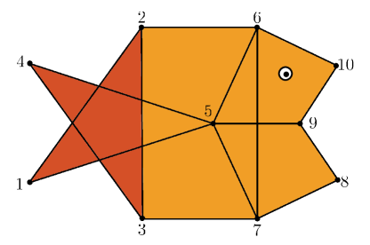
Figure 1. Fig. 4 in [9]

In [12], the authors extend the above example from [9] by showing two claw-free graphs called “fish in a net” and “fish in a net with bubble” each with a facet inequality that has several different non-zero coefficients. Both normals appear in $\mathcal{A}_{G}^{(2)}$. We illustrate the “fish in a net with bubble” case. Let $G$ be the complement of the graph shown in Figure 2. Then $\textup{STAB}(G)$ has the following facet inequality [12]:

$$3x_{1}+3x_{2}+3x_{3}+3x_{4}+4x_{5}+4x_{6}+4x_{7}+5x_{8}+4x_{9}$$

$$+5x_{10}+5x_{11}+4x_{12}+6x_{13}+2x_{14}+2x_{15}+2x_{16}+6x_{17} \leq 8$$

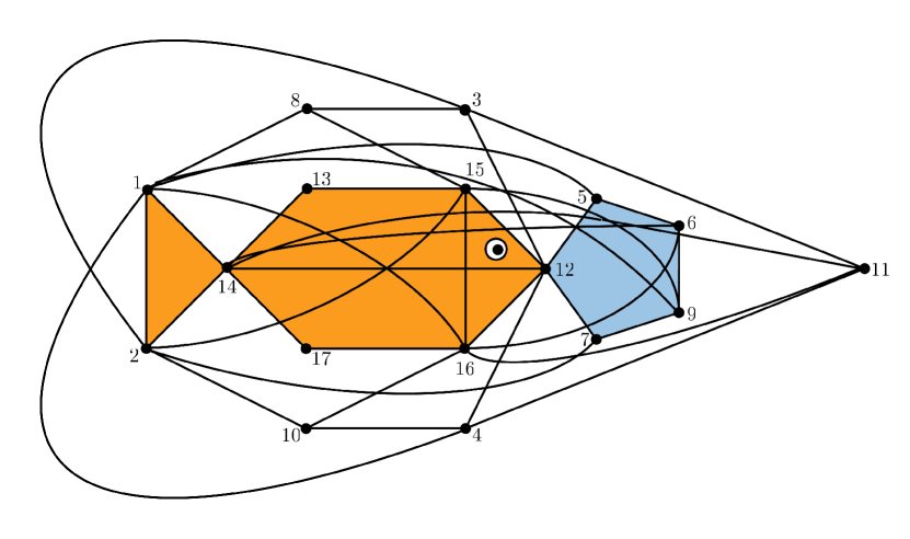
Figure 2. Fish in a net with bubble

Let ${\mathcal{B}}$ be the rows of the following $17\times 17$ matrix $B$.

$$\left(\begin{array}[]{c c c c c c c c c c c c c | r r r r}\mathbf{1}&1&1&1&0&1&1&1&1&1&1&0&\mathbf{1}&1&1&1&1\\ \mathbf{1}&\mathbf{1}&1&1&1&0&1&1&0&1&1&1&1&1&1&1&1\\ 1&\mathbf{1}&\mathbf{1}&1&1&1&0&1&1&1&1&0&1&1&1&1&1\\ 0&1&\mathbf{1}&\mathbf{1}&1&1&1&1&1&1&1&1&1&0&0&0&1\\ 1&0&1&\mathbf{1}&\mathbf{1}&1&1&1&1&1&1&1&1&0&0&0&1\\ 1&1&0&1&\mathbf{1}&\mathbf{1}&1&1&1&1&1&1&1&0&0&0&1\\ 1&1&1&0&1&\mathbf{1}&\mathbf{1}&1&1&1&1&1&1&0&0&0&1\\ 0&0&0&0&1&1&\mathbf{1}&\mathbf{1}&0&1&1&1&1&0&0&0&1\\ 0&0&0&0&0&0&0&\mathbf{1}&\mathbf{1}&0&0&1&1&0&0&0&1\\ 0&0&0&0&0&0&0&0&\mathbf{1}&\mathbf{1}&0&0&0&0&0&0&1\\ 0&0&0&0&1&1&1&1&1&\mathbf{1}&\mathbf{1}&0&1&0&0&0&1\\ 0&0&0&0&0&0&0&0&0&0&\mathbf{1}&\mathbf{1}&1&0&0&0&0\\ 0&0&0&0&0&0&0&0&0&0&0&\mathbf{1}&\mathbf{1}&0&0&0&1\\ \hline\cr 0&0&0&0&0&0&0&0&0&0&0&0&0&\mathbf{-1}&0&0&0\\ 0&0&0&0&0&0&0&0&0&0&0&0&0&0&\mathbf{-1}&0&0\\ 0&0&0&0&0&0&0&0&0&0&0&0&0&0&0&\mathbf{-1}&0\\ 0&0&0&0&0&0&0&0&0&0&0&0&0&0&0&0&\mathbf{-1}\\ \end{array}\right)$$

Then ${\bf{b}}_{1},\ldots,{\bf{b}}_{13}$ are characteristic vectors of odd circuits in $G$. We denote the consecutive vertices in one such odd circuit for each ${\bf{b}}_{i}$ in the table below.

$$\begin{array}[]{ll}{\bf{b}}_{1}&1,3,4,2,6,7,8,9,10,11,13,16,14,15,17\\ {\bf{b}}_{2}&1,3,2,5,4,7,8,10,11,12,13,16,14,15,17\\ {\bf{b}}_{3}&1,3,2,5,4,6,8,9,10,11,15,14,16,13,17\\ {\bf{b}}_{4}&2,3,4,5,7,6,8,9,10,11,12,13,17\\ {\bf{b}}_{5}&1,3,4,5,7,6,8,9,10,11,12,13,17\\ {\bf{b}}_{6}&1,4,2,5,7,6,8,9,10,11,12,13,17\\ {\bf{b}}_{7}&1,3,2,5,7,6,8,9,10,11,12,13,17\\ {\bf{b}}_{8}&5,7,6,8,10,11,12,13,17\\ {\bf{b}}_{9}&8,9,12,13,17\\ {\bf{b}}_{10}&9,10,17\\ {\bf{b}}_{11}&5,7,6,8,9,10,11,13,17\\ {\bf{b}}_{12}&11,12,13,11\\ {\bf{b}}_{13}&12,13,17,12\end{array}$$

Therefore, ${\mathcal{B}}\subset\mathcal{A}_{G}^{(1)}$ and check that $\textup{det}(B)=18$, hence, ${\mathcal{B}}$ is a basis. It can be verified using a Hilbert basis package such as Normaliz [5] that the normal v from the facet inequality above is in $\textup{Hilb}({\mathcal{B}})$:

$${\bf{v}}=\left(\frac{2}{3},\frac{2}{3},\frac{2}{3},\frac{1}{3},\frac{1}{3},\frac{1}{3},\frac{1}{3},\frac{2}{3},\frac{1}{3},\frac{1}{3},\frac{2}{3},\frac{1}{3},\frac{2}{3},0,0,0,0\right)B,$$

which proves that ${\bf{v}}\in\mathcal{A}_{G}^{(2)}$. The hypercycle associated with ${\mathcal{B}}$ is indicated by the bold $1$’s in the matrix $B$.

It is a long-standing open problem to give a complete linear inequality description of $\textup{STAB}(G)$ when $G$ is a claw-free graph. The following would be a step toward settling this problem.

Problem 4.11.

Is $\textup{SCR}(\textup{FRAC}(G))\leq 2$ for all claw-free graphs $G$?

We now derive various corollaries to Theorem 4.9.

Corollary 4.12.

The normals of all clique inequalities lie in $\mathcal{A}_{G}^{(2)}$.

Proof:   Corollary 4.3 showed that the normals of all odd clique inequalities lie in $\mathcal{A}_{G}^{(1)}$. Suppose $H$ is an even clique in $G$ with vertex set $V_{H}$. For $i,j\in V_{H}$, let $C_{i}$ be an odd circuit through all vertices of $V_{H}$ except $i$ and similarly, $C_{j}$ be an odd circuit through all vertices of $V_{H}$ except $j$. Then ${\bf{e}}(C_{i}),{\bf{e}}(C_{j})$ and ${\bf{e}}_{i}+{\bf{e}}_{j}$ are all present in $\mathcal{A}_{G}^{(1)}$ by Proposition 4.1. The odd circuits $C_{i},C_{j}$ and the edge $\{i,j\}$ together form a triangle in the hypergraph $G^{\prime}$, and the vectors ${\bf{e}}(C_{i}),{\bf{e}}(C_{j})$ and ${\bf{e}}_{i}+{\bf{e}}_{j}$ are linearly independent since for any $k\in V_{H}\setminus\{i,j\}$, the $3\times 3$ submatrix indexed by $i,j,k$, of the $3\times n$ matrix whose rows are these three vectors is non-singular. Dividing the sum of the three vectors by $2$ produces ${\bf{e}}(H)$. This vector is in the minimal Hilbert basis of the cone spanned by ${\bf{e}}(C_{i}),{\bf{e}}(C_{j})$ and ${\bf{e}}_{i}+{\bf{e}}_{j}$ since its restriction $(1,1,1)$ to the coordinates indexed by $i,j,k$ is in the minimal Hilbert basis of the cone spanned by the same restriction of ${\bf{e}}(C_{i}),{\bf{e}}(C_{j})$ and ${\bf{e}}_{i}+{\bf{e}}_{j}$. Since ${\bf{e}}(C_{i})$, ${\bf{e}}(C_{j})$, ${\bf{e}}_{i}+{\bf{e}}_{j}$ can be extended to a basis in $\mathcal{A}_{G}^{(1)}$, the result follows. $\square$

Definition 4.13.

1. A graph $G=([n],E)$ is perfect if $\textup{STAB}(G)$ is cut out by the non-negativity and clique inequalities.

2. A graph $G=([n],E)$ is h-perfect if $\textup{STAB}(G)$ is cut out by the non-negativity, odd circuit and clique inequalities.

All perfect graphs are $h$-perfect. Many well-known classes of graphs such as bipartite, comparability and chordal graphs are perfect [18].

Corollary 4.14.

If $G$ is h-perfect then $\textup{SCR}(\textup{FRAC}(G))=2$.

If $H$ is a subgraph of $G$, then note that the configuration $\mathcal{A}_{H}^{(0)}$ is a subset of $\mathcal{A}_{G}^{(0)}$ after padding all coordinates corresponding to vertices of $G$ that are not in $H$ by zeros. This implies that $\mathcal{A}_{H}^{(k)}$ is also a subset of $\mathcal{A}_{G}^{(k)}$, for any positive integer $k$, after the same padding by zeros. Therefore, if we need to show that a facet normal of $\textup{STAB}(G)$ whose support lies in the vertices of $H$ appears in $\mathcal{A}_{G}^{(k)}$, then it suffices to show that it appears in $\mathcal{A}_{H}^{(k)}$.

Corollary 4.15.

Normals of antihole and odd wheel inequalities appear in $\mathcal{A}_{G}^{(2)}$.

Proof:   By the above discussion, we may assume without loss of generality that $G$ is an antihole. Since the vertices of an odd antihole support an odd circuit, its characteristic vector appears in $\mathcal{A}_{G}^{(1)}$. If $G$ is an even antihole, then $G$ contains $n$ odd circuits each going through all vertices of $G$ except one. The $n\times n$ matrix $B$ whose rows are the characteristic vectors of these odd circuits has all diagonal entries equal to zero and all off-diagonal entries equal to one. Since $B$ is non-singular, its rows form a basis in $\mathcal{A}_{G}^{(1)}$. Dividing the sum of the rows of $B$ by $n-1$ produces ${\bf{e}}(G)$, which is the unique new element in the minimal Hilbert basis of $\textup{cone}({\mathcal{B}})$.

Again assume without loss of generality that $G$ is an odd wheel with central vertex $u_{0}$ and remaining vertices $u_{1},\cdots,u_{2k-1}$. Let $B$ be the $2k\times 2k$ matrix whose rows are the characteristic vectors of the $2k-1$ triangles in $G$ and $-{\bf{e}}_{0}$. Then $B$ is non-singular and that half the sum of its rows is the normal of the odd wheel inequality.

$$\left(\begin{array}[]{r r r r r r r }1&1&1&0&0&\ldots&0\\ 1&0&1&1&0&\ldots&0\\ 1&0&0&1&1&\ldots&0\\ &&&&&\ddots&\\ 1&1&0&0&0&\ldots&1\\ -1&0&0&0&0&\ldots&0\end{array}\right)$$

The $2k-1$ triangles are the hyperedges that form an odd cycle in $G^{\prime}$ which underlies this normal. $\square$

Recall that the line graph, $L(G)$, of a graph $G=(V,E)$ is the graph $L(G)=(E,F)$ where $\{e,e^{\prime}\}\in F$, for $e,e^{\prime}\in E$, if and only if $e$ and $e^{\prime}$ share a vertex in $G$. A complete linear description of $\textup{STAB}(L(G))$ was given by Edmonds as follows (see [17, p. 440]):

$$\textup{STAB}(L(G))=\left\{{\bf{x}}\in\mathbb{R}^{E}\,:\,\begin{array}[]{ll}x_{e}\geq 0&\forall\,\,e\in E\\ \sum_{v\in e}x_{e}\leq 1&\forall\,\,v\in V\\ \sum_{e\in E[U]}x_{e}\leq\lfloor\frac{|U|}{2}\rfloor&\forall\,\,U\subseteq V,\,|U|\,\,\textup{odd}\end{array}\right\},$$

where $E[U]$ denotes the edges in $E$ that have both end points in $U$. Note that the second class of inequalities in the description of $\textup{STAB}(L(G))$ are clique inequalities.

Corollary 4.16.

For any graph $G$, $\textup{SCR}(\textup{FRAC}(L(G)))\leq 3$.

Proof:   It is known that $\textup{STAB}(L(G))$ is the first Chvátal closure of the polytope described by the clique and non-negativity constraints from $L(G)$. Since clique normals are in $\mathcal{A}_{L(G)}^{(2)}$, it follows that $\textup{SCR}(\textup{FRAC}(L(G)))\leq 3$. $\square$

5. Lower bounds

In this section we establish lower bounds on SCR in various situations. We also discuss computational evidence that supports possible upper bounds in some of these cases. Note that by Proposition 2.6, a lower bound on the SCR or Chvátal rank of a system $A{\bf{x}}\leq{\bf{b}}$ is also a lower bound on the corresponding rank of $A$. On the other hand, an upper bound on either rank of $A$ is an upper bound on the corresponding rank of $A{\bf{x}}\leq{\bf{b}}$ for any ${\bf{b}}$.

Theorem 5.1.

For $m,n\geq 3$, the small Chvátal rank of $A{\bf{x}}\leq{\bf{b}}$ (and hence of $A$) can grow exponentially in the size of the input.

In proving Theorem 5.1, we may assume $m=n=3$. All other cases follow by adjoining inequalities that do not affect Chvátal rank or SCR. Let $j\geq 2$ be arbitrary and set

$$A=\left(\begin{array}[]{ccc}1&0&0\\ 0&1&0\\ 1&j&2j-1\end{array}\right).$$

We will show that the SCR of $A$ is $j-1$ which is exponential in the bit size of $A$. To do this, we explicitly describe $\mathcal{A}^{(k)}$ for all $k$ and prove that $\mathcal{A}^{(j-1)}=\mathcal{A}^{(j)}$, so the SCR of $A$ is at most $j-1$. Then we identify a vector in $\mathcal{A}^{(j-1)}\setminus\mathcal{A}^{(j-2)}$ that is a facet normal of an integer hull $Q_{{\bf{b}}}^{I}$.

For $1\,\leq\,k\,\leq\,j-1$, define an integral polygon

$$R^{k} := \textup{conv}\{(0,0),(k+1,k+1),(j,2j-1-k),(j,2j-1)\}\subseteq\mathbb{R}^{2}_{\geq 0}$$

$$= \{(x,y)\in\mathbb{R}^{2}:\;x\leq y,\;2x\leq y+k+1,\;x\leq j,\;y\leq\left(\frac{2j-1}{j}\right)x\}.$$

For $k=j-1$, the second and third points in the convex hull description coincide; for $k<j-1$ the four points are distinct and in convex position.

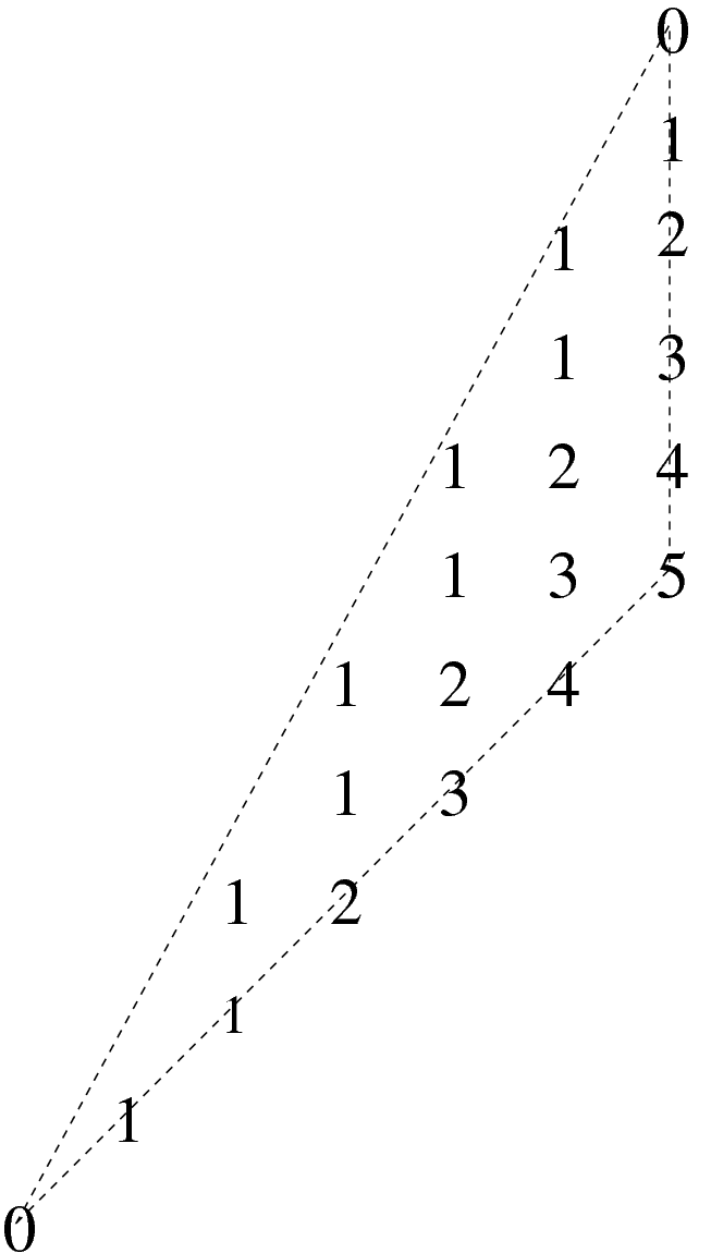
Figure 3. The polygon $R^{j-1}$ (with $j=6$) used to prove Theorem 5.1. Each integer point $(a,b)$ in the polygon is labeled by the smallest $k$ such that $(1,a,b)$ appears in $\mathcal{A}_{6}^{(k)}$.

Lemma 5.2.

[11, Proposition 5.1] Let $R$ be an integral polygon in $\mathbb{R}^{2}$. The configuration $\{(1,a,b):\,(a,b)\in R\cap\mathbb{Z}^{2}\}$ is supernormal.

Lemma 5.3.

For $1\leq k\leq j-1$,

$$\mathcal{A}^{(k)}=\{(0,1,0)\}\cup\{(1,a,b):\,(a,b)\in R^{k}\cap\mathbb{Z}^{2}\}.$$

Proof:   Induct on $k$. For $k=1$, we have

$$R^{1}=\{(x,y)\in\mathbb{R}^{2}:\;x\leq y,\;2x\leq y+2,\;x\leq j,\;y\leq\left(\frac{2j-1}{j}\right)x\}$$

and it is easy to check that

$$R^{1}\cap\mathbb{Z}^{2}=\{(0,0)\}\cup\{(i,2i-1)\,:\,1\leq i\leq j\}\cup\{(i,2i-2)\,:\,2\leq i\leq j\}.$$

Observe that

$$(1,i,2i-1)=\left(\frac{2j-2i}{2j-1},\frac{j-i}{2j-1},\frac{2i-1}{2j-1}\right)A$$

for $1\leq i\leq j$ and that

$$(1,i,2i-2)=\left(\frac{2j-2i+1}{2j-1},\frac{2j-i}{2j-1},\frac{2i-2}{2j-1}\right)A$$

for $2\leq i\leq j$, so all the points in $\{1\}\times(R^{1}\cap\mathbb{Z}^{2})$ are in the fundamental parallelepiped of $\mathcal{A}$. Since all the first coordinates are one, no element of $\{1\}\times R^{1}\cap\mathbb{Z}^{2}$ is a sum of others. Also, no two elements of $\{1\}\times R^{1}\cap\mathbb{Z}^{2}$ differ by a multiple of $(0,1,0)$. Thus $\{1\}\times(R^{1}\cap\mathbb{Z}^{2})\subseteq\textup{Hilb}(\mathcal{A})\subseteq\mathcal{A}^{(1)}.$

On the other hand, if $h=c_{1}(1,0,0)+c_{2}(0,1,0)+c_{3}(1,j,2j-1)$ is an integer point in the fundamental parallelepiped of $\mathcal{A}$ (so $0\leq c_{1},c_{2},c_{3}<1$), then $c_{3}=\frac{p}{2j-1}$ for some integer $1\leq p\leq 2j-2$ and $c_{1}$ and $c_{2}$ are uniquely determined by $c_{3}$, so $h$ must be one of the listed points in $R^{1}\cap\mathbb{Z}^{2}$.

For the induction step, first assume that $\mathcal{A}^{(k-1)}$ contains $\{1\}\times R^{k-1}\cap\mathbb{Z}^{2}$ for some $k\geq 2$. The difference between $R^{k-1}$ and $R^{k}$ is that the inequality $2x\leq y+k$ is relaxed to $2x\leq y+k+1$. So we must show that the new vectors in $\mathcal{A}^{(k)}$ include

(2) $$\{(1,k+i,k+2i-1):1\,\leq i\,\leq j-k\}.$$

For each $1\,\leq\,i\,\leq\,j-k$, the three vectors $(0,1,0)$, $(1,k+i-1,k+2i-2)$, and $(1,k+i,k+2i)$ appear in $\mathcal{A}^{(k-1)}$ by the induction hypothesis. The basis cone $C$ that they span has normalized volume two, and $(1,k+i,k+2i-1)$ (half the sum of the three vectors) is the unique integer point in the interior of the fundamental parallelepiped. Thus $(1,k+i,k+2i-1)\in\textup{Hilb}(C)\subseteq\mathcal{A}^{(k)}.$

Next assume for some $k$ that $\mathcal{A}^{(k-1)}$ contains no other vectors. By Lemma 5.2, the previous paragraph, and the induction hypothesis, the set

$$\mathcal{A}_{j}^{(k-1)}\setminus\{(0,1,0)\}\;=\;R^{k}\cap\mathbb{Z}^{2}$$

is supernormal. Thus the only bases of $\mathcal{A}^{(k-1)}$ that might contribute new vectors to $\mathcal{A}^{(k)}$ are those that include $(0,1,0).$ Any new vector obtained this way would be of the form $(1,a,b)$ for $(a-1,b)$ strictly in the interior of $R^{k-1}$ and $(a,b)$ outside $R^{k-1}$. From the inequality description of $R^{k-1}$, this vector must indeed be of the form (2); see Figure 3. $\square$

Lemma 5.4.

The configuration $\mathcal{A}^{(j-1)}$ is supernormal.

Proof:   By the same argument as above, any vector ${\bf{v}}\in\mathcal{A}^{(j)}\setminus\mathcal{A}^{(j-1)}$ is of the form $(1,a,b)$ for $(a-1,b)$ in the interior of $R^{j-1}$ and $(a,b)$ outside $R^{j-1}$. However, $R^{j-1}$ is a triangle whose right boundary consists only of segments of the line $y=x$ and of the line $x\leq j$, so no such $(a,b)$ exists. Thus $\mathcal{A}^{(j)}=\mathcal{A}^{(j-1)}$. $\square$

Proof of Theorem 5.1: By Lemma 5.3, we have $(1,j,j)^{t}\in\mathcal{A}^{(j-1)}\setminus\mathcal{A}^{(j-2)}$. So it will suffice to show that the inequality

(3) $$(1,j,j)\,{\bf{x}}\,\leq\,{\bf 0}$$

defines a facet of the integer hull

$$P_{j}:=\{{\bf{x}}\in\mathbb{R}^{3}\,:\,A{\bf{x}}\,\leq\,(0,0,j-1)^{t}\}^{I}.$$

Let ${\bf{y}}=(y_{1},y_{2},y_{3})\in Q_{(0,0,j-1)^{t}}\cap\mathbb{Z}^{3}$. We first show that ${\bf{y}}$ satisfies  (3). If $y_{3}\leq 0$, then since we already know $y_{1},y_{2}\leq 0$, immediately ${\bf{y}}$ satisfies  (3). If $y_{3}=1$ and $y_{2}\leq-1$, again ${\bf{y}}$ satisfies  (3). If $y_{3}=1$ and $y_{2}=0$, then to satisfy the last inequality in $A{\bf{x}}\leq(0,0,j-1)^{t}$, $y_{1}\leq-j$ and again ${\bf{y}}$ satisfies  (3).

Finally, suppose $y_{3}\geq 2$. Rewrite $x_{1}+jx_{2}+(2j-1)x_{3}\,\leq\,j-1$ as

(4) $$x_{1}+jx_{2}\,\leq\,(j-1)-x_{3}(2j-1).$$

Then

$$\begin{array}[]{ccccc}(1,j,j)\,{\bf{y}}&=&y_{1}+jy_{2}+jy_{3}&\leq&(j-1)-y_{3}(2j-1)+jy_{3}\\ &=&j+y_{3}(1-j)-1&\leq&j+2(1-j)-1\\ &=&1-j&<&0\end{array}$$

where the first inequality follows from (4), the second from $y_{3}\geq 2$, and the last from $j\geq 2$. Thus the inequality (3) is valid on all integer points of $Q_{(0,0,j-1)^{t}}$ and hence on $P_{j}$.

To finish the proof we must argue that  (3) is a facet inequality of $P_{j}$. This follows from the observation that the three affinely independent integer points $(0,-1,1)^{t}$, $(0,0,0)^{t}$, and $(-j,0,1)^{t}$ in $P_{j}$ satisfy  (3) with equality. $\square$

Many optimization problems are modeled as $0/1$ integer programs, in which case the starting linear programming relaxation is a polytope in the unit cube $C_{n}=[0,1]^{n}.$ For such polytopes, it is known that Chvátal rank is bounded above by $n^{2}(1+\log n)$, and there are examples with Chvátal rank at least $(1+\epsilon)n$ [7]. We will derive a lower bound for SCR of the same order, using quite different techniques.

Theorem 5.5.

There are systems $A{\bf{x}}\leq{\bf{b}}$ defining polytopes contained in the unit cube $C_{n}$ whose small Chvátal ranks are at least $n/2-o(n)$.

Observation 5.6.

If ${\bf{v}}\in\textup{Hilb}(\{{\bf{v}}_{1},\ldots,{\bf{v}}_{n}\})$, then $\|{\bf{v}}\|_{\infty}<n(\textup{max}_{i}\|{\bf{v}}_{i}\|_{\infty})$ since ${\bf{v}}=\sum_{i=1}^{n}\lambda_{i}{\bf{v}}_{i}$ for $0\leq\lambda_{i}<1$, $i=1,\ldots,n$.

Proof of Theorem 5.5: Given any 0/1 polytope $Q$, we can find a relaxation $P$ contained in $C_{n}$ and whose facet normals are 0/1/-1 vectors. For instance, for any $U\subseteq[n]$, the inequality

$$\sum_{i\in U}x_{i}-\sum_{i\notin U}x_{i}\;\leq\;\left|U\right|-1$$

is violated by ${\bf{e}}(U)$ but satisfied by every other vertex of $C_{n}$. Define $P$ by starting with $C_{n}$ and adjoining such an inequality for each vertex of $C_{n}$ that is not in $Q$.

Using a construction by Alon and Vu [1] of 0/1 matrices with large determinants, Ziegler [22, Corollary 26] constructs an $n$-dimensional 0/1 polytope $Q$ with a (relatively prime integer) facet normal ${\bf{v}}$ whose $\infty$-norm is at least $\frac{(n-1)^{(n-1)/2}}{2^{2n+o(n)}}.$ Let $P$ be as above for this $Q$, and let $k$ be the SCR of the system $A{\bf{x}}\leq{\bf{b}}$ defining $P$. By definition, ${\bf{v}}\in\mathcal{A}^{(k)}$. Since $\mathcal{A}$ consists entirely of 0/1/-1 vectors, we get by repeatedly applying Observation 5.6 that

$$n^{k}>\frac{(n-1)^{(n-1)/2}}{2^{2n+o(n)}}.$$

Taking the logarithm of both sides, we see that

$$k\log n > \left(\frac{n-1}{2}\right)\log(n-1)-(2n+o(n))\log 2$$

$$= \frac{n}{2}\log(n-1)-\frac{1}{2}\log(n-1)-2n\log 2-o(n)$$

$$= \frac{n}{2}\log n-o(n\log n)$$

$$= (\frac{n}{2}-o(n))\log n$$

so $k>n/2-o(n)$ as claimed. $\square$

It would be very interesting to find an upper bound for the SCR of any polytope in $C_{n}$ that improves the ${\mathcal{O}}(n^{2}\,\textup{log}\,n)$ upper bound on Chvátal rank in [7]. Our experiments in dimension up to $7$ suggest that there might be a uniform upper bound for the SCR of any polytope in $C_{n}$ of order ${\mathcal{O}}(n)$. Facet normals of $0/1$ $n$-polytopes with large coefficients (matching the Alon-Vu bound) for $n\leq 10$ can be found in the Polymake database at http://www.math.tu-berlin.de/polymake/. We have confirmed that for $n\leq 7$, these facet normals appear in two rounds of IBN applied to the normals of the standard relaxation of a $0/1$-polytope in $C_{n}$ used in the proof of Theorem 5.5. For instance, when $n=7$, the Polymake database shows that $(9,7,5,3,2,1,1)$ is a possible facet normal. This vector lies in the minimal Hilbert basis of the basis cone spanned by the vectors:

$$(3,2,2,2,1,0,0),(3,2,2,0,0,0,0),(3,2,1,0,0,0,0),(2,2,1,1,1,1,1),$$

$$(2,2,1,1,1,1,0),(2,2,1,1,1,0,1),(2,2,1,1,0,0,0)$$

which are all found in the first round of IBN applied to $\{\pm 1\}^{7}$.

The fractional stable set polytope $\textup{FRAC}(G)$ of a graph $G=([n],E)$ examined in Section 4 lies in the unit cube $C_{n}$. We will now derive a lower bound depending on $n$, for $\textup{SCR}(\textup{FRAC}(G))$ as $G$ varies over all graphs with $n$ vertices. This result contrasts the many examples of normals shown in Section 4 for which SCR is at most two. We rely on a construction found in [13] for producing facet normals of $\textup{STAB}(G)$ with large coefficients.

Definition 5.7.

The product graph of $G_{1}=(V_{1},E_{1})$ and $G_{2}=(V_{2},E_{2})$ is the graph $G=(V,E)$ where $V=V_{1}\cup V_{2}$ and $E=E_{1}\cup E_{2}\cup\{uv\,:\,u\in V_{1},v\in V_{2}\}$.

Lemma 5.8.

Suppose $G_{i}=(V_{i},E_{i})$, $i=1,2$ are graphs such that the inequality $\sum_{u\in V_{i}}a_{i}(u)x_{u}\leq b_{i}$ defines a facet of $\textup{STAB}(G_{i})$ with ${\bf{a}}_{i}:=(a_{i}(u))$ primitive for $i=1,2$. The inequality

$$b_{2}(\sum_{u\in V_{1}}a_{1}(u)x_{u})+b_{1}(\sum_{u\in V_{2}}a_{2}(u)x_{u})\leq b_{1}b_{2}$$

is facet-defining for $\textup{STAB}(G)$. If $(b_{1},b_{2})=1$ then the facet normal shown above is primitive.

Observation 5.9.

By Observation 5.6, for $G=([n],E)$, if ${\bf{v}}\in\mathcal{A}_{G}^{(k)}$, then $||{\bf{v}}||_{\infty}\leq n^{k}$. Therefore, if $\textup{STAB}(G)$ has a primitive facet normal ${\bf{a}}\in\mathbb{Z}^{n}$, then $\textup{SCR}(\textup{FRAC}(G))\geq\lfloor\textup{log}_{n}||{\bf{a}}||_{\infty}\rfloor$.

Theorem 5.10.

There is no constant $t$ such that $\textup{SCR}(\textup{FRAC}(G))\leq t$ for all graphs $G$.

Proof:   Let $k_{1},k_{2},\ldots,k_{p}$ be the first $p$ prime numbers and consider the odd cycles $C_{2k_{i}+1}$ for $i=1,\ldots,p$. In each case, the odd hole inequality $\sum_{j=1}^{2k_{i}+1}x_{j}\leq k_{i}$ is facet-defining for $\textup{STAB}(C_{2k_{i}+1})$. Let $G_{p}$ be the product graph $C_{5}\times C_{7}\times C_{11}\times\cdots C_{2k_{p}+1}$ which has $2(\sum_{i=1}^{p}k_{i})+p$ vertices. By Lemma 5.8, there is a primitive facet normal of $\textup{STAB}(G_{p})$ with infinity norm $\prod_{i=1}^{p}k_{i}$.

The sum of the first $p$ prime numbers, $\sum_{i=1}^{p}k_{i}$ is approximately $\frac{1}{2}p^{2}\textup{ln}p$ [2],and hence the number of vertices of $G_{p}$ is approximately $p^{2}\,\textup{ln}\,p+p<p^{2+\epsilon}$. On the other hand, $\prod_{i=1}^{p}k_{i}$ is asymptotically $e^{(1+o(1))p\ln p}>e^{p\ln p}$. Therefore, $\textup{SCR}(\textup{FRAC}(G_{p}))\geq\textup{log}_{p^{2+\epsilon}}e^{p\ln p}=\frac{p}{2+\epsilon}$, asymptotically. $\square$

Problem 5.11.

Is it true that for $G=([n],E)$, $\textup{SCR}(\textup{FRAC}(G))\leq n$? More generally, is there an upper bound of order ${\mathcal{O}}(n)$ for the SCR of any polytope in the unit cube $C_{n}$?

If the answer to the above problem is yes, then SCR would become comparable to the number of steps needed by the modern lift and project methods for finding the integer hull of a polytope in $C_{n}$ such as those in [4], [14] and [20], since these methods take at most $n$ steps. There are a few different observations that support a positive answer. For instance, it was shown in [21] that the semidefinite operator $N_{+}$ in [14] takes $\lfloor n/2\rfloor$ iterations to produce $\textup{STAB}(G)$ from $\textup{FRAC}(G)$ when $G$ is the line graph of $K_{n}$ with $n$ odd. By Corollary 4.16, $\textup{SCR}(\textup{FRAC}(G))\leq 3$ for any line graph $G$. For the operator $N$, it was shown in [14] that $N(\textup{FRAC}(G))=Q_{G}^{(1)}$, the first Chvátal closure of $\textup{FRAC}(G)$. Comparing with the small Chvátal closure, we get that $N^{0}(\textup{FRAC}(G))=\textup{FRAC}(G)=S_{G}^{(0)}$ and $N^{1}(\textup{FRAC}(G)=Q_{G}^{(1)}\supseteq S_{G}^{(1)}$. If this pattern continues and we get $N^{k}(\textup{FRAC}(G))\supseteq S_{G}^{(k)}$ for all $k\geq 2$, then indeed, $\textup{SCR}(\textup{FRAC}(G))$ would be at most $n$ when $G$ has $n$ vertices.

Acknowledgments. We thank Sasha Barvinok, Ravi Kannan and Les Trotter for helpful inputs to this paper.

References

- [1] Alon. N., Vu, V.: Anti-Hadamard matrices, coin weighing, threshold gates and indecomposable hypergraphs. J. Combin Theory Ser. A 79(1), 133–160 (1997)
- [2] Bach, E., Shallit, J.: Algorithmic Number Theory, Volume 1: Efficient Algorithms. Foundations of Computing Series, MIT Press, Cambridge, MA (1996)
- [3] Barvinok, A., Woods, K.: Short rational generating functions for lattice point problems. J. Amer. Math. Soc 16, 957–979 (2003)
- [4] Balas, E., Ceria, S., Cornuéjols, G.: A lift-and-project cutting plane algorithm for mixed 0-1 programs. Mathematical Programming 58, 295–324 (1993)
- [5] Bruns, W., and Ichim, B.: NORMALIZ. Computing normalizations of affine semigroups. With contributions by C. Söger. Available at http://www.math.uos.de/normaliz.
- [6] Chvátal, V.: Edmonds polytopes and a hierarchy of combinatorial problems. Discrete Mathematics 4, 305–337 (1973)
- [7] Eisenbrand, F., Schulz, A.S.: Bounds on the Chvátal rank of polytopes in the 0/1 cube. Combinatorica, 23(2), 245–261 (2003)
- [8] Galluccio, A., Sassano, A.: The rank facets of the stable set polytope for claw-free graphs. J. Combin. Theory Ser. B 69(1), 1–38 (1997)
- [9] Giles, R., and Trotter, L.E. Jr.: On stable set polyhedra for -free graphs. J. Combin. Theory Ser. B 31(3), 313–326 (1981)
- [10] Grötschel, M., Lovász, L., Schrijver, A.: Geometric algorithms and combinatorial optimization. Volume 2 of Algorithms and Combinatorics. Springer-Verlag, Berlin, second edition (1993)
- [11] Hoşten, S., Maclagan, D., Sturmfels, B.: Supernormal vector configurations. J. Algebraic Combinatorics 19(3), 297–313 (2004)
- [12] Liebling, T.M., Oriolo, G., Spille, B., Stauffer, G.: On non-rank facets of the stable set polytope of claw-free graphs and circulant graphs. Math. Methods Oper. Res. 59(1), 25–35 (2004)
- [13] Lipták, L., Lovász, L.: Facets with fixed defect of the stable set polytope. Math. Program. 88(1, Ser. A), 33–44 (2000)
- [14] Lovász, L., Schrijver, A.: Cones of matrices and set-functions and - optimization. SIAM J. Optim. 1(2), 166–190 (1991)
- [15] Maclagan, D., Thomas, R.R.: The toric Hilbert scheme of a rank two lattice is smooth and irreducible. J. Combin. Theory Ser. A 104, 29–48 (2003)
- [16] Schrijver, A.: Theory of Linear and Integer Programming. Wiley-Interscience Series in Discrete Mathematics and Optimization, New York (1986)
- [17] Schrijver, A.: Combinatorial optimization. Polyhedra and efficiency. Vol. A, volume 24 of Algorithms and Combinatorics. Springer-Verlag, Berlin (2003) Paths, flows, matchings, Chapters 1–38.
- [18] Schrijver, A.: Combinatorial optimization. Polyhedra and efficiency. Vol. A, volume 24 of Algorithms and Combinatorics. Springer-Verlag, Berlin (2003) Matroids, trees, stable sets, Chapters 39–69.
- [19] Seymour, P.D.: Decomposition of regular matroids. J. Combin. Theory Ser. B 28(3), 305–359 (1980)
- [20] Sherali, H.D., Adams, W.P.: A hierarchy of relaxations between the continuous and convex hull representations for zero-one programming problems. SIAM J. Discrete Math 3(3), 411–430 (1990)
- [21] Stephen, T., Tunçel, L.: On a representation of the matching polytope via semidefinite liftings. Math. Oper. Res. 24(1), 1–7 (1999)
- [22] Ziegler, G.M.: Lectures on -polytopes. In: Polytopes—combinatorics and computation, Oberwolfach, 1997, volume 29 of DMV Sem, pp. 1–41. Birkhäuser, Basel (2000)