Particle-vibration coupling within covariant density functional theory

Abstract

Covariant density functional theory, which has so far been applied only within the framework of static and time dependent mean field theory is extended to include Particle-Vibration Coupling (PVC) in a consistent way. Starting from a conventional energy functional we calculate the low-lying collective vibrations in Relativistic Random Phase Approximation (RRPA) and construct an energy dependent self-energy for the Dyson equation. The resulting Bethe-Salpeter equation in the particle-hole ($ph$) channel is solved in the Time Blocking Approximation (TBA). No additional parameters are used and double counting is avoided by a proper subtraction method. The same energy functional, i.e. the same set of coupling constants, generates the Dirac-Hartree single-particle spectrum, the static part of the residual $ph$-interaction and the particle-phonon coupling vertices. Therefore a fully consistent description of nuclear excited states is developed. This method is applied for an investigation of damping phenomena in the spherical nuclei with closed shells ²⁰⁸Pb and ¹³²Sn. Since the phonon coupling terms enrich the RRPA spectrum with a multitude of $ph\otimes$phonon components a noticeable fragmentation of the giant resonances is found, which is in full agreement with experimental data and with results of the semi-phenomenological non-relativistic approach.

I Introduction

The theoretical analysis of nuclear dynamics by microscopic methods remains undoubtedly a crucial issue of present-day nuclear physics. Besides the merely theoretical interest it is stimulated by new experimental opportunities for the study of the nuclear many-body system. Along with new possibilities to investigate more precisely nuclear systems being considered well known, the recent generation of radioactive-beam facilities enables us to examine exotic systems with extreme spin and isospin values. For a successful description of nuclei close to the limits of stability a powerful and reliable theory should be provided. It should be based on a consistent treatment of both ground and excited states and it should allow for predictions of nuclear properties in areas, which are hard or impossible to access by future experiments.

Ab initio calculations and multi-configuration mixing within the shell-model can, so far, only be applied in light nuclei. At present, for a universal description of nuclei all over the periodic table, Density Functional Theory (DFT) based on the mean-field concept provides a very reasonable concept. DFT has been introduced in the sixties in atomic and molecular physics HK.64 ; KS.65 and shortly after that in nuclear physics, where it has been called density dependent Hartree-Fock theory VB.72 ; DG.80 . Today it is widely used for all kinds of quantum mechanical many-body systems. Density functional theory can, in principle, provide an exact description of the many-body dynamics, if the exact density functional is known, but for such systems as nuclei one is far from a microscopic derivation and one is forced to determine the functional in a phenomenological way. Starting from basic symmetries the parameters are adjusted to characteristic experimental data in finite nuclei and nuclear matter.

One of the most successful schemes of this type is Covariant Density Functional Theory (CDFT). It is based on Lorentz invariance connecting in a consistent way the spin and spatial degrees of freedom in the nucleus. Therefore, it needs only a relatively small number of parameters which are adjusted to reproduce a set of bulk properties of spherical closed-shell nuclei Rin.96 ; VALR.05 . A large variety of nuclear phenomena have been described over the years within this kind of model: ground state properties of finite spherical and deformed nuclei all over the periodic table GRT.90 from light nuclei LVR.04a to super-heavy elements LSRG.96 ; BBM.04 , from the neutron drip line, where halo phenomena are observed MR.96 , to the proton drip line LVR.04 with nuclei unstable against the emission of protons LVR.99 . Rotational bands are treated within the relativistic cranking approximation KR.89 ; ARK.00 and the Relativistic Random Phase Approximation (RRPA) RMG.01 and quasi-particle RRPA PRN.03 have been formulated as the small amplitude limit of time-dependent Relativistic Mean-Field (RMF) models for a description of collective and non-collective excitations. This method is successful, in particular, for the description of the positions of giant resonances and spin/isospin-excitations as the Isobaric Analog Resonance (IAR) or the Gamow-Teller Resonance (GTR) PNV.04 . Recently it has been also used for a theoretical interpretation of low-lying dipole PRN.03 and quadrupole Ans.05 excitations.

With a few exceptions, where the quadrupole motion has been studied within the relativistic Generator Coordinate Method (GCM) NVR.06 , applications of covariant density functional theory to the description of excited states are limited to relativistic RPA, i.e. to configurations of $1p1h$-nature. None of these methods, however, can be applied to the investigation of the coupling to more complicated configurations, as it occurs for instance in the damping phenomena causing the width of giant resonances. It is also known, that in such theories, because of the low values of the effective mass, the level density of the single-particle spectrum in the vicinity of the Fermi surface is considerably reduced as compared to the experimental data.

Based on the Fermi Liquid Theory (FLT) of Landau Lan.59 the Theory of Finite Fermi Systems (TFFS) of Migdal Mig.67 is another very successful method for the description of low-lying nuclear excitations RSp.74 , which is known since the fifties. It has several general properties in common with density functional theory. First, both theories are know to be exact, at least in principle, but in practice the parameters entering these theories have to be determined in a phenomenological way by adjustment to experimental data. Second, both theories are based in some sense on a single-particle concept. Density functional theory uses the mean field concept with Slater determinants in an effective single-particle potential as a vehicle to introduce shell-effects in an exact theory and Fermi liquid theory is based on the concept of quasi-particles obeying a Dyson equation, which are defined as the basic excitations of the neighboring system with odd particle number. Third, in practical applications both theories describe in the simplest versions the nuclear excitations in the RPA approximation, i.e. by a linear combination of $ph$-configurations in an average nuclear potential.

However, there are also essential differences between these two concepts. First, in contrast to DFT, TFFS does not attempt to calculate the ground state properties of the many-body system, but it describes the nuclear excitations in terms of Landau quasi-particles and their interaction. Therefore the experimental data used to fix the phenomenological parameters of the theories are bulk properties of the ground state in the case of density functional theory, and properties of single-particle excitations and of the collective excitations in the case of finite Fermi systems theory. Second, in DFT the mean field is determined in a self-consistent way and therefore the RPA spectrum contains Goldstone modes at zero energy. This is usually not the case in TFFS calculations, which are based on a non-relativistic shell-model potential, whose parameters are adjusted to the experimental single-particle spectra. Therefore there is no self-consistency in the RPA calculations of TFFS and the Goldstone modes do not separate from the other modes. They are distributed among the low-lying excitations. Third, modern versions of TFFS go much beyond the mean field approximation. Using Green’s function techniques the coupling between quasi-particles and phonons has been investigated. Based on the phonons calculated in the framework of the RPA one has included particle-phonon coupling vertices and an energy dependence of the self-energy in the Dyson equation RW.73 ; HS.76 . This leads also to an induced interaction in the Bethe-Salpeter equation caused by the exchange of phonons which also depends on the energy. The coupling of particles and phonons has also been derived from Nuclear Field Theory (NFT) and its extensions BM.75 ; BBB.77 ; BBB.85 . Many aspects of the coupling between the quasi-particles and the collective vibrations have been investigated with these techniques BBBD.79 ; BB.81 ; CBGBB.92 ; CB.01 ; SBC.04 ; Tse.89 ; KTT.97 ; KST.04 ; Tse.05 ; LT.05 as well as with other kinds of approaches beyond RPA Sol ; DNSW.90 over the years.

The present work makes the attempt to find a combination of the basic ideas of density functional theory and Landau-Migdal theory. The concept is similar to earlier work in Refs. KS.79 ; KS.80 ; FTT.00 , where specific non-relativistic energy functionals have been used to construct Self-Consistent Theory of Finite Fermi Systems. We start here from a covariant density functional $E[\rho]$ widely used in the literature. It is adjusted to ground state properties of characteristic nuclei and, without any additional parameter, it provides the necessary input of finite Fermi systems theory, such as the mean field and the single-particle spectrum as well as an effective interaction between the $ph$-configurations in terms of the second derivative of the same energy $E[\rho]$ with respect to the density. Thus the phenomenological input of Landau-Migdal theory is replaced by the results of density functional theory. The same interaction is used to calculate the vertices for particle-vibration coupling LR.06 . We then apply the techniques of Landau-Migdal theory and its modern extensions to describe vibrational coupling and complex configurations. In this way we obtain a fully consistent description of the many-body dynamics.

Two essential approximations are used in this context: First, the Time-Blocking Approximation (TBA) blocks in a special time-projection technique the $1p1h$-propagation through states which have a more complex structure than $1p1h\otimes$phonon. The nuclear response can then be explicitly calculated on the $1p1h+1p1h\otimes$phonon level by summation of an infinite series of Feynman’s diagrams. This approximation has been introduced in Ref. Tse.89 . Initially it was called Method of Chronological Decoupling of Diagrams (MCDD) and it is also discussed in recent review articles KTT.97 ; KST.04 . Second, a special subtraction technique guarantees, that there is no double counting between the additional correlations introduced by particle-vibration coupling and the ground state correlations already taken into account in the phenomenological density functional. These two tools are essential for the success of the present method. TBA introduces a consistent truncation scheme into the Bethe-Salpeter equation and without it it would be hard to solve the equations explicitly. The subtraction method is the essential tool to connect density functional theory so far used only on the level of mean field theory, i.e. on the RPA level, with the extended Landau-Migdal theory, where complex configurations are included through particle-vibration coupling.

As discussed above there are several versions of density functional theory in nuclear system. In the present work we use covariant density functional theory with the parameter set NL3 NL3 . A first attempt in this direction has been carried out in Ref. LR.06 , where we treated the level density problem in the framework of covariant particle-vibration coupling.

In Section II we discuss shortly the general formalism of covariant density functional theory, we introduce the concept of the energy dependent self-energy $\Sigma(\varepsilon)$ and the vertices of particle-vibration coupling in the relativistic framework, and we discuss the response formalism and the time blocking approximation for the response function. In Section III we show, how to solve the resulting integral equations in detail and present recent numerical applications for the spreading width of the doubly magic nuclei ²⁰⁸Pb and ¹³²Sn and in Section IV we include a brief summary and an outlook for future applications. Appendices A-D provide some more details for the formalism used in the calculations.

II Formalism

II.1 The relativistic mean-field approach

In relativistic mean-field theory the nucleus is considered as a system of nucleons interacting by the exchange of effective mesons, which characterize the quantum numbers of the various fields. Conventional RMF theory uses $\sigma$, $\omega$ and $\rho$-mesons and the photon as a minimal set of bosons which is necessary to generate realistic nuclear fields Wal.74 ; SW.86 ; Rin.96 . This concept is expressed by the following Lagrangian density depending on the nucleon spinor $\psi$ as well as on the mesons $\sigma$, $\omega^{\mu}$, ${\vec{\rho}}^{\mu}$ and the electromagnetic fields $A^{\mu}$ :

$$\mathcal{L} ={\bar{\psi}}(i\gamma^{\mu}\partial_{\mu}-m)\psi+\frac{1}{2}\partial^{\mu}\sigma\partial_{\mu}\sigma-\frac{1}{2}m_{\sigma}^{2}\sigma^{2}$$

$$-\frac{1}{4}\Omega^{\mu\nu}\Omega_{\mu\nu}+\frac{1}{2}m_{\omega}^{2}\omega^{\mu}\omega_{\mu}-\frac{1}{4}{\vec{R}}^{\mu\nu}{\vec{R}}_{\mu\nu}+\frac{1}{2}m_{\rho}^{2}{\vec{\rho}}^{\ \mu}{\vec{\rho}}_{\mu}-\frac{1}{4}F^{\mu\nu}F_{\mu\nu}$$

$$-{\bar{\psi}}\Bigl{(}{\Gamma}_{\sigma}\sigma+\Gamma_{\omega}^{\mu}\omega_{\mu}+{\vec{\Gamma}}_{\rho}^{\ \mu}{\vec{\rho}}_{\mu}+\Gamma_{e}^{\mu}A_{\mu}\Bigr{)}\psi.$$ (1)

Here $m$ is the bare nucleon mass, $m_{\sigma}$, $m_{\omega}$ and $m_{\rho}$ are the corresponding meson masses, and $\Omega_{\mu\nu}$, ${\vec{R}}_{\mu\nu},F_{\mu\nu}$ are field tensors:

$$\Omega_{\mu\nu} =\partial_{\mu}\omega_{\nu}-\partial_{\nu}\omega_{\mu}\ ,$$

$${\vec{R}}_{\mu\nu} =\partial_{\mu}{\vec{\rho}}_{\nu}-\partial_{\nu}{\vec{\rho}}_{\mu}\ ,$$

$$F_{\mu\nu} =\partial_{\mu}A_{\nu}-\partial_{\nu}A_{\mu}.$$ (2)

As usual arrows denote isovectors and boldface symbols will be used for vectors in ordinary space. The vertices $\Gamma$ entering the interaction term of Eq. (1) read

$$\Gamma_{\sigma}=g_{\sigma},\ \ \ \ \Gamma_{\omega}^{\mu}=g_{\omega}\gamma^{\mu},\ \ \ \ {\vec{\Gamma}}_{\rho}^{\ \mu}=g_{\rho}{\vec{\tau}}\gamma^{\mu},\ \ \ \ \Gamma_{e}^{\mu}=e\frac{(1-\tau_{3})}{2}\gamma^{\mu},$$ (3)

where $g_{\sigma}$, $g_{\omega}$, $g_{\rho}$ and $e$ are the corresponding coupling constants. For the sake of simplicity, we use in the following discussions the linear version (1) of the Lagrangian. However, it is well known that one needs an additional density dependence in order to obtain a reliable description of nuclear surface properties. It is either expressed by a non-linear self-interaction between the mesons or by an explicit density dependence of the coupling constants $g_{\sigma}$, $g_{\omega}$, and $g_{\rho}$. In all the numerical applications we use such modifications. They are discussed in detail in Appendix A.

The classical variation principle being applied to the Lagrangian density (1) leads to the following system of coupled equations of motion for the Fermions

$$(i\gamma^{\mu}\partial_{\mu}-m-\sum\limits_{m}\Gamma_{m}\phi_{m}(\mathbf{r},t))\psi_{i}(\mathbf{r},t)=0$$ (4)

and the mesons:

$$(\Box+m_{m}^{2})\phi_{m}(\mathbf{r},t))=\mp\sum\limits_{i}{\bar{\psi}}_{i}(\mathbf{r},t)\Gamma_{m}{\psi}_{i}(\mathbf{r},t).$$ (5)

Here the index $i$ numerates the nucleons and the index $m=\{\sigma,\omega,\rho,e\}$ runs over the set of meson fields $\phi_{m}=\{\sigma,\omega^{\mu},{\vec{\rho}}^{\mu},A^{\mu}\}$. $m_{m}$ are the corresponding masses and $\Gamma_{m}$ are the vertices (3). The $-$sign in Eq. (5) holds for scalar fields and the $+$sign for vector fields. The set of Eqs. (4) and (5) defines the standard RMF model. It implies the following four approximations:

i) only the motion of the nucleons is quantized, the meson and electromagnetic degrees of freedom are described by classical fields. The nucleons move independently in these classical fields, i.e. residual two-body correlations are disregarded and the many-nucleon wave function is a Slater determinant at all times.

ii) in time-dependent applications we use the instantaneous approximation, i.e. the time derivatives $\partial_{t}^{2}$ in the Klein-Gordon equations and consequently the retardation effects for the meson fields are neglected although the Dirac spinors $\psi_{i}$ as well as the fields $\phi_{m}$ are functions of coordinates and time. This is justified by the relatively large meson masses and the corresponding short range of the meson exchange interaction.

iii) Fock terms are neglected. Because of the short range character of the meson exchange forces they behave similar to zero range forces, where the Fock terms have the same form as the direct terms and contribute only in a change of the relevant strength parameters. Since our strength parameters are adjusted to experiment, Fock terms for the heavy mesons are implicitly taken into account to a large extend.

iv) the no-sea approximation means, that nucleon states in the Dirac sea with negative energies do not contribute to the densities and currents: the sum over $i$ in the Eq. (5) includes only occupied levels with positive energy in the Fermi sea. This means we do not consider vacuum polarization explicitly. Since our parameters are adjusted to experimental data such effects are taken into account in an implicit way.

II.2 The energy-dependent nucleon self-energy

Let us now consider in detail the Dyson equation, which describes the motion of a single nucleon in the nuclear interior:

$$(i\gamma^{\mu}\partial_{\mu}-m-\Sigma)\psi_{i}=0.$$ (6)

Here the total self-energy $\Sigma$ contains all the forces acting on the nucleon. As long as one stays within RMF approach the nucleon self-energy contains only static and local contributions from the mesons and from the electromagnetic fields.

When we go beyond the mean-field approximation, we have to take into account that in the general case the full self-energy $\Sigma$ is non-local in the space coordinates as well as in time. This non-locality means that its Fourier transform has both momentum and energy dependence. Let us now decompose the total self-energy matrix into two components, a static local and an energy dependent non-local term:

$$\Sigma(\mathbf{r},\mathbf{r^{\prime}};\varepsilon)={\tilde{\Sigma}}(\mathbf{r})\delta(\mathbf{r}-\mathbf{r^{\prime}})+\Sigma^{e}(\mathbf{r},\mathbf{r^{\prime}};\varepsilon),$$ (7)

where

$${\tilde{\Sigma}}(\mathbf{r})=\sum\limits_{m}\Gamma_{m}\phi_{m}(\mathbf{r})$$ (8)

is the static part known from RMF theory in Eq. (4). The upper index ”e” in $\Sigma^{e}$ indicates the energy dependence. The Dyson equation for single-particle Green’s function reads:

$$(\varepsilon-h^{\mathcal{D}}-\beta\Sigma^{e}(\varepsilon))G(\varepsilon)=\beta,$$ (9)

where $h^{\mathcal{D}}$ denotes the Dirac hamiltonian in Eq. (4) with the energy-independent mean field:

$$h^{\mathcal{D}}={\mbox{\boldmath$\alpha$}}\mathbf{p}+\beta(m+{\tilde{\Sigma}}_{s})+{\tilde{\Sigma}}_{0},\ \ \ \ \ {\mbox{\boldmath$\alpha$}}=\beta{\mbox{\boldmath$\gamma$}},\ \ \ \beta=\gamma^{0}.$$ (10)

Most of the static calculations are done for cases, where time-reversal symmetry is valid. In all these cases there are no currents in the nucleus and, thus, only scalar ${\tilde{\Sigma}}_{s}$ and time-like ${\tilde{\Sigma}}_{0}$ components of ${\tilde{\Sigma}}$ survive in the static Dirac hamiltonian of Eq. (10). In the shell-model Dirac basis $\{|\psi_{k}\rangle\}$ which diagonalizes the energy-independent part of the Dirac equation

$$h^{\mathcal{D}}|\psi_{k}\rangle=\varepsilon_{k}|\psi_{k}\rangle$$ (11)

one can rewrite Eq. (9) as follows:

$$\sum\limits_{l}\bigl{\{}(\varepsilon-\varepsilon_{k})\delta_{kl}-\Sigma_{kl}^{e}(\varepsilon)\bigr{\}}G_{lk^{\prime}}(\varepsilon)=\delta_{kk^{\prime}},$$ (12)

where

$$\Sigma_{kl}^{e}(\varepsilon)=\int d^{3}rd^{3}{r}^{\prime}~{}\bar{\psi}_{k}(\mbox{\boldmath$r$})\Sigma^{e}({\mbox{\boldmath$r$}},{\mbox{\boldmath$r$}^{\prime}};\varepsilon)\psi_{l}({\mbox{\boldmath$r$}^{\prime}})\,,$$ (13)

$$G_{kl}(\varepsilon)=\int d^{3}rd^{3}{r}^{\prime}~{}\bar{\psi}_{k}(\mbox{\boldmath$r$})\,\beta G({\mbox{\boldmath$r$}},{\mbox{\boldmath$r$}^{\prime}};\varepsilon)\beta\,\psi_{l}({\mbox{\boldmath$r$}^{\prime}})\,.$$ (14)

The letter indices $k,k^{\prime},l$ denote full sets of the single-particle quantum numbers. In the present work we consider spherical symmetry, so that the spinor $|\psi_{k}\rangle$ is characterized by the set $k=\{(k),m_{k}\}$ and $(k)=\{n_{k},j_{k},\pi_{k},{\tau}_{k}\}$ with the radial quantum number $n_{k}$, angular momentum quantum numbers $j_{k},m_{k}$, parity $\pi_{k}$ and isospin ${\tau}_{k}$:

$$\psi_{k}(\mathbf{r},s,t)=\left(\begin{array}[c]{c}f_{(k)}(r)\Phi_{l_{k}j_{k}m_{k}}(\vartheta,\varphi,s)\\ ig_{(k)}(r)\Phi_{{\tilde{l}}_{k}j_{k}m_{k}}(\vartheta,\varphi,s)\end{array}\right)\chi_{{\tau}_{k}}(t),$$ (15)

where $s$ and $t$ are the coordinates for spin and isospin. The orbital angular momenta $l_{k}$ and $\tilde{l}_{k}$ of the large and small components are determined by the parity of the state $k$:

$$\left\{\begin{array}[c]{ccc}l_{k}=j_{k}+\frac{1}{2},&{\tilde{l}}_{k}=j_{k}-\frac{1}{2}&\mbox{for}\ \ \pi_{k}=(-1)^{j_{k}+\frac{1}{2}}\\ l_{k}=j_{k}-\frac{1}{2},&{\tilde{l}}_{k}=j_{k}+\frac{1}{2}&\mbox{for}\ \ \pi_{k}=(-1)^{j_{k}-\frac{1}{2}},\end{array}\right.$$ (16)

$f_{(k)}(r)$ and $g_{(k)}(r)$ are radial wave functions and $\Phi_{ljm}(\vartheta,\varphi,s)$ is a two-dimensional spinor:

$$\Phi_{ljm}(\vartheta,\varphi,s)=\sum\limits_{m_{s}m_{l}}({\frac{{\scriptstyle 1}}{{\scriptstyle 2}}}m_{s}lm_{l}|jm)Y_{lm_{l}}(\vartheta,\varphi)\chi_{m_{s}}(s).$$ (17)

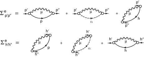
Figure 1: The particle $\Sigma^{e}_{p^{\prime}p^{\prime\prime}}$ and the hole $\Sigma^{e}_{h^{\prime}h^{\prime\prime}}$ components of the relativistic mass operator in the graphical representation. Solid and dashed lines with arrows denote one-body propagators for particle ($p$), hole ($h$), and antiparticle ($\alpha$) states. Wavy lines denote phonon ($\mu$) propagators, empty circles are the particle-phonon coupling amplitudes $\gamma^{\mu}$. See text for the detailed explanation.

As in Ref. LR.06 we use the particle-phonon coupling model for the energy dependent part of the self-energy $\Sigma^{e}(\varepsilon)$. In the Dirac basis of the spinors $|\psi_{k}\rangle$ defined in Eq. (11) it has the form

$$\Sigma_{kl}^{e}(\varepsilon)=\sum\limits_{\mu,n}\frac{\gamma_{kn}^{\mu(\sigma_{n})}\,\gamma_{ln}^{\mu(\sigma_{n})\ast}}{\varepsilon-\varepsilon_{n}-\sigma_{n}(\Omega^{\mu}-i\eta)},\qquad\gamma_{kn}^{\mu(\sigma)}=\delta_{\sigma,+1}^{\vphantom{A}}\gamma_{kn}^{\mu}+\delta_{\sigma,-1}^{\vphantom{A}}\gamma_{nk}^{\mu\ast}\ ,$$ (18)

where $\eta\rightarrow+0$. In Fig. 1 we show a graphical representation for $\Sigma_{kl}^{e}(\varepsilon)$. The index $n$ runs over all single-particle states in this basis. We distinguish occupied states in the Fermi sea $|h\rangle$ (hole states) with $\sigma_{h}=-1$, unoccupied states above the Fermi level $|p\rangle$ (particle states) with $\sigma_{p}=+1$, and states in the Dirac sea $|\alpha\rangle$ (anti-particle states) with negative energies. Due to the no-sea approximation the orbits with negative energies $|\alpha\rangle$ are left unoccupied and therefore we have $\sigma_{\alpha}=+1$. However, as it has been shown in Ref. LR.06 the numerical contribution of the diagrams with intermediate states $\alpha$ with negative energy is very small due to the large energy denominators in the corresponding terms of the self-energy (18). The index $\mu$ in Eq. (18) labels the various phonons taken into account. $\Omega^{\mu}$ is their frequency, ${\rho}^{\mu}$ is their transition density and the phonon vertices $\gamma_{kl}^{\mu}$ determine their coupling to the nucleons:

$$\gamma_{kl}^{\mu}=\sum\limits_{k^{\prime}l^{\prime}}\tilde{V}_{kl^{\prime},lk^{\prime}}^{\vphantom{A}}{\rho}_{k^{\prime}l^{\prime}}^{\mu}.$$ (19)

$\tilde{V}_{kl^{\prime},lk^{\prime}}$ denotes the relativistic matrix element of the residual interaction. It is a obtained as functional derivative of the relativistic mean field with respect to relativistic density matrix ${\rho}$

$$\tilde{V}_{kl^{\prime},lk^{\prime}}=\frac{\delta{\tilde{\Sigma}}_{l^{\prime}k^{\prime}}}{\delta\rho_{lk}}.$$ (20)

We use the linearized version of the model which assumes that $\rho^{\mu}$ is not influenced by the particle-phonon coupling and can be computed within the relativistic RPA approximation. As long as we neglect the non-linear self-couplings of the mesons or the density dependence of the coupling constants $g_{m}$ in Eq. (3) the matrix elements $\tilde{V}_{kl^{\prime},lk^{\prime}}^{\vphantom{A}}$ in Eq. (19) have simple Yukawa form. However, such effects have to be taken into account to guarantee full self-consistency of the RRPA equations and we find more complicated expressions, which are discussed in detail in Appendix A. In the applications investigated in section III we use the non-linear parameter set NL3 NL3 for the solution of the static Dirac equation (11) as well as for the calculation of the matrix elements (20).

II.3 The response function

Nuclear dynamics of an even-even nucleus in a weak external field is described by the linear response function $R(14,23)$ which is the solution of the Bethe-Salpeter equation (BSE) in the $ph$ channel. In the beginning it is convenient to consider this equation in the time representation. Let us include the time variable into the single-particle indices setting $1=\{k_{1},t_{1}\}$. In this notation the Bethe-Salpeter equation BSE for the response function $R$ reads:

$$R(14,23)=G(1,3)G(4,2)-i\sum\limits_{5678}G(1,5)G(6,2)V(58,67)R(74,83),$$ (21)

where the summation over the number indices $1$, $2,\dots$ implies integration over the respective time variables. The function $G$ is the exact single-particle Green’s function, and $V$ is the amplitude of the effective interaction irreducible in the $ph$-channel. This amplitude is determined as a variational derivative of the full self-energy $\Sigma$ with respect to the exact single-particle Green’s function:

$$V(14,23)=i\frac{\delta\Sigma(4,3)}{\delta G(2,1)}.$$ (22)

Introducing the free response $R^{0}(14,23)=G(1,3)G(4,2)$ the Bethe-Salpeter equation (21) can be written in a shorthand notation as

$$R=R^{0}-iR^{0}VR.$$ (23)

For the sake of simplicity, we will use this shorthand notation frequently in the following discussions. Since the self-energy in Eq. (7) has two parts $\Sigma=\tilde{\Sigma}+\Sigma^{e}$, the effective interaction $V$ in Eq. (21) is a sum of the static RMF interaction $\tilde{V}$ and time-dependent terms $V^{e}$:

$$V=\tilde{V}+V^{e},$$ (24)

where (with $t_{12}=t_{1}-t_{2}$)

$$\tilde{V}(14,23)=\tilde{V}_{k_{1}k_{4},k_{2}k_{3}}\delta(t_{31})\delta(t_{21})\delta(t_{34})$$ (25)

is the static part of the interaction (see Eq. (20)) and

$$V^{e}(14,23)=i\frac{\delta{\Sigma^{e}(4,3)}}{\delta G(2,1)}$$ (26)

contains the energy dependence. In the space of the Dirac basis  (11) the amplitude $V^{e}$ has the form:

$$V_{kl^{\prime},lk^{\prime}}^{e}(\omega,\varepsilon,\varepsilon^{\prime})=\sum\limits_{\mu,\sigma}\frac{\sigma\gamma_{k^{\prime}k}^{\mu(\sigma)\ast}\gamma_{l^{\prime}l}^{\mu(\sigma)}}{\varepsilon-\varepsilon^{\prime}+\sigma(\Omega^{\mu}-i\eta)}.$$ (27)

In order to make the Bethe-Salpeter equation (21) more convenient for the further analysis we eliminate the exact Green’s function $G$ and rewrite it in terms of the mean field Green’s function $\tilde{G}$:

$${\tilde{G}}(1,2)=-i\sigma_{k_{1}}\delta_{k_{1}k_{2}}\theta(\sigma_{k_{1}}\tau)e^{-i\varepsilon_{k_{1}}\tau},\ \ \ \ \ \tau=t_{1}-t_{2},$$ (28)

where $\theta(t)$ is the Heaviside function. After a Fourier transformation in time this reads

$${\tilde{G}}_{k_{1}k_{2}}(\varepsilon)=\frac{\delta_{k_{1}k_{2}}}{\varepsilon-\varepsilon_{k_{1}}+i\sigma_{k_{1}}\eta}.$$ (29)

Using the connection between $\tilde{G}$ and $G$ in the Nambu form

$${\tilde{G}}^{-1}(1,2)=G^{-1}(1,2)+\Sigma^{e}(1,2),$$ (30)

one can rewrite Eq. (21) as follows:

$$R={\tilde{R}}^{0}-i\tilde{R}^{0}WR,$$ (31)

with ${\tilde{R}}^{0}(14,23)={\tilde{G}}(1,3){\tilde{G}}(4,2)$ and $W$ is a new interaction of the form

$$W=\tilde{V}+W^{e}$$ (32)

where

$$W^{e}(14,23)=V^{e}(14,23)+i\Sigma^{e}(1,3){\tilde{G}}^{-1}(4,2)+i{\tilde{G}}^{-1}(1,3)\Sigma^{e}(4,2)-i\Sigma^{e}(1,3)\Sigma^{e}(4,2).$$ (33)

Since the mean field Green’s function ${\tilde{G}}$ in Eq. (29) is known one has a more convenient starting point for the solution of the Bethe-Salpeter equation (31) than with the unknown exact single-particle Green’s function, but the effective interaction $W$ in Eq. (32) becomes more complicated. The graphical representation of the Eq. (31) is shown in Fig. 2.

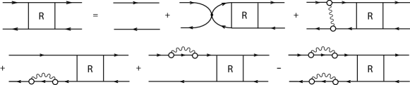
Figure 2: Bethe-Salpeter equation for the $ph$-response function $R$ in graphical representation. Details are given in Fig. 1 and the small black circle means the static part of the residual $ph$-interaction (20).

In addition to the static interaction $\tilde{V}$ the effective interaction $W$ contains diagrams with energy dependent self-energies and an energy dependent induced interaction, where a phonon is exchanged between the particle and the hole. Here and hereinafter we omit the term $i\Sigma^{e}(3,1)\Sigma^{e}(2,4)$ in the Eq. (33) by the following reasons. This term compensates the multiple counting of the particle-phonon coupling arising from the two previous terms in the Eq. (33). However, this multiple counting does not take place within time blocking approximation (see below) if the backward-going propagators are not taken into account. Components containing the backward-going propagators within $1p1h\otimes$phonon configurations require a special consideration. They have been analyzed in great detail in the Refs. Tse.89 ; KTT.97 ; KST.04 . In the present work they are fully neglected and therefore the term $i\Sigma^{e}(3,1)\Sigma^{e}(2,4)$ has also to be omitted. However, we have to emphasize, that we only neglect ground state correlations (backward-going diagrams) caused by the particle-phonon coupling. All the RPA ground state correlations are taken into account, because it is well known that they play a central role for the conservation of currents and sum rules. We consider that this is a reasonable approximation which is applied and discussed also in many non-relativistic models (see e.g. Refs. BBBD.79 ; BB.81 ; CBGBB.92 ; CB.01 ; SBC.04 ; Tse.89 ; KTT.97 ; KST.04 ; Tse.05 ; LT.05 and references therein).

Considering a Fourier transformation of the Bethe-Salpeter equation (31) in time

$$R_{k_{1}k_{4},k_{2}k_{3}}(\omega,\varepsilon) ={\tilde{G}}_{k_{1}k_{3}}(\varepsilon+\omega){\tilde{G}}_{k_{4}k_{2}}(\varepsilon)$$

$$+\sum\limits_{k_{5}k_{6}k_{7}k_{8}}{\tilde{G}}_{k_{1}k_{5}}(\varepsilon+\omega){\tilde{G}}_{k_{6}k_{2}}(\varepsilon)\int\limits_{-\infty}^{\infty}\frac{d\varepsilon^{\prime}}{2\pi i}W_{k_{5}k_{8},k_{6}k_{7}}(\omega,\varepsilon,\varepsilon^{\prime})R_{k_{7}k_{4},k_{8}k_{3}}(\omega,\varepsilon^{\prime}),$$ (34)

one finds that both the solution of this equation $R$ and its kernel $W$ are singular with respect to the energy variables. Another difficulty arises because Eq. (31) contains integrations over all time points of the intermediate states. This means that many configurations which are actually more complex than $1p1h\otimes$phonon are contained in the exact response function. In the Ref. Tse.89 a special time-projection technique was introduced to block the $ph$-propagation through these complex intermediate states. It has been shown that for this type of response it is possible to reduce the integral equation (34) to a relatively simple algebraic equation. Obviously, this method can be applied straightforwardly in our case too.

Starting from the Bethe-Salpeter equation (31) we divide the problem to find the exact response function into two parts. First we calculate the correlated propagator $R^{e}$ which describes the propagation under the influence of the interaction $W^{e}$

$$R^{e}={\tilde{R}}^{0}-i{\tilde{R}}^{0}W^{e}R^{e}.$$ (35)

It contains all the effects of particle-phonon coupling and all the singularities of the integral part of the initial BSE. Second, we have to solve the remaining equation for the full response function $R$

$$R=R^{e}-iR^{e}\tilde{V}R.$$ (36)

Eq. (36) contains only the static effective interaction $\tilde{V}$ and can be easily solved if $R^{e}$ is known. Thus, the main problem is to calculate the correlated propagator $R^{e}$ .

II.4 Time blocking approximation (TBA) and subtraction method

In order to calculate the correlated propagator $R^{e}$ we represent this quantity as an infinite series of graphs which contain mean field $ph$-propagators alternated with single interaction acts. This can be expressed by the system of the following equations:

$$R^{e} ={\tilde{R}}^{0}-i{\tilde{R}}^{0}{\Gamma}^{e}{\tilde{R}}^{0},$$ (37)

$${\Gamma}^{e} =W^{e}-iW^{e}{\tilde{R}}^{0}{\Gamma}^{e}.$$ (38)

According to the main idea of the time blocking approximation we modify the integral part of Eq. (38) making use of the time-projection operator in the form Tse.89 :

$$\Theta(14,23)=\delta_{\sigma_{k_{1}},-\sigma_{k_{2}}}\delta_{k_{1}k_{3}}\delta_{k_{2}k_{4}}\theta(\sigma_{k_{1}}t_{14})\theta(\sigma_{k_{1}}t_{23}),$$ (39)

where $\theta(t)$ is the Heaviside function. This projection operator is introduced into the mean field propagator $\tilde{R}^{0}$ in the integral part of the Eq. (38) to order the $ph$-propagation in time and, thus, to separate in time the acts of the particle-phonon interaction from each other and to exclude configurations which are more complex than $1p1h\otimes$phonon. We replace in Eq. (38) the mean field propagator $\tilde{R}^{0}$ by

$$\tilde{R}^{0}(14,23)\rightarrow\tilde{R}^{0}(14,23)\Theta(14,23)$$ (40)

and obtain instead of Eq. (38)

$${\Gamma}^{e}(14,23)=W^{e}(14,23)+\frac{1}{i}\sum\limits_{5678}W^{e}(16,25){\tilde{R}}^{0}(58,67)\Theta(58,67){\Gamma}^{e}(74,83).$$ (41)

After a Fourier transformation in time we restrict ourselves to the response function $R_{k_{1}k_{4},k_{2}k_{3}}(\omega)$

$$R_{k_{1}k_{4},k_{2}k_{3}}(\omega)=-i\int\limits_{-\infty}^{\infty}dt_{1}dt_{2}dt_{3}dt_{4}\delta(t_{1}-t_{2})\delta(t_{3}-t_{4})\delta(t_{4})e^{i\omega t_{13}}R(14,23),$$ (42)

which depends only on one energy variable $\omega$.

The time projection by the operator (39) leads to a separation of integrations in Eq. (34) and we find an algebraic equation for the function (42):

$$R_{k_{1}k_{4},k_{2}k_{3}}(\omega)=\tilde{R}_{k_{1}k_{4},k_{2}k_{3}}^{0}(\omega)+\sum\limits_{k_{5}k_{6}k_{7}k_{8}}\tilde{R}_{k_{1}k_{6},k_{2}k_{5}}^{0}(\omega){\bar{W}}_{k_{5}k_{8},k_{6}k_{7}}(\omega)R_{k_{7}k_{4},k_{8}k_{3}}(\omega),$$ (43)

or in shorthand notation

$$R(\omega)=\tilde{R}^{0}(\omega)+\tilde{R}^{0}(\omega){\bar{W}}(\omega)R(\omega),$$ (44)

where

$${\bar{W}}_{k_{1}k_{4},k_{2}k_{3}}(\omega)=\tilde{V}_{k_{1}k_{4},k_{2}k_{3}}+\Phi_{k_{1}k_{4},k_{2}k_{3}}(\omega)$$ (45)

and

$${\tilde{R}}_{k_{1}k_{4},k_{2}k_{3}}^{0}(\omega)={\tilde{R}}_{k_{1}k_{2}}(\omega)\delta_{k_{1}k_{3}}\delta_{k_{2}k_{4}}.$$ (46)

${\tilde{R}}_{k_{1}k_{2}}(\omega)$ is the mean field propagator:

$${\tilde{R}}_{ph}(\omega) =-\frac{1}{\varepsilon_{ph}-\omega},\ \ \ \ {\tilde{R}}_{{\alpha}h}(\omega)=-\frac{1}{\varepsilon_{{\alpha}h}-\omega},$$ (47)

$${\tilde{R}}_{hp}(\omega) =-\frac{1}{\varepsilon_{ph}+\omega},\ \ \ \ {\tilde{R}}_{h{\alpha}}(\omega)=-\frac{1}{\varepsilon_{{\alpha}h}+\omega},$$ (48)

$\varepsilon_{ph}=\varepsilon_{p}-\varepsilon_{h}$ and $\Phi$ is the particle-phonon coupling amplitude with the following components:

$$\Phi_{ph^{\prime},hp^{\prime}}(\omega) =\sum\limits_{\mu}\Bigl{[}\delta_{pp^{\prime}}\sum\limits_{h^{\prime\prime}}\frac{\gamma_{h^{\prime\prime}h}^{\mu}\gamma_{h^{\prime\prime}h^{\prime}}^{\mu\ast}}{\omega-\varepsilon_{p}+\varepsilon_{h^{\prime\prime}}-\Omega^{\mu}}$$

$$+\delta_{hh^{\prime}}\Bigl{(}\sum\limits_{p^{\prime\prime}}\frac{\gamma_{pp^{\prime\prime}}^{\mu}\gamma_{p^{\prime}p^{\prime\prime}}^{\mu\ast}}{\omega-\varepsilon_{p^{\prime\prime}}+\varepsilon_{h}-\Omega^{\mu}}+\sum\limits_{{\alpha}^{\prime\prime}}\frac{\gamma_{p{\alpha}^{\prime\prime}}^{\mu}\gamma_{p^{\prime}{\alpha}^{\prime\prime}}^{\mu\ast}}{\omega-\varepsilon_{{\alpha}^{\prime\prime}}+\varepsilon_{h}-\Omega^{\mu}}\Bigr{)}$$

$$-\Bigl{(}\frac{\gamma_{pp^{\prime}}^{\mu}\gamma_{hh^{\prime}}^{\mu\ast}}{\omega-\varepsilon_{p^{\prime}}+\varepsilon_{h}-\Omega^{\mu}}+\frac{\gamma_{p^{\prime}p}^{\mu\ast}\gamma_{h^{\prime}h}^{\mu}}{\omega-\varepsilon_{p}+\varepsilon_{h^{\prime}}-\Omega^{\mu}}\Bigr{)}\Bigr{]},$$ (49)

$$\Phi_{\alpha h^{\prime},h\alpha^{\prime}}(\omega) =\sum\limits_{\mu}\Bigl{[}\delta_{\alpha\alpha^{\prime}}\sum\limits_{h^{\prime\prime}}\frac{\gamma_{h^{\prime\prime}h}^{\mu}\gamma_{h^{\prime\prime}h^{\prime}}^{\mu\ast}}{\omega-\varepsilon_{\alpha}+\varepsilon_{h^{\prime\prime}}-\Omega^{\mu}}$$

$$+\delta_{hh^{\prime}}\Bigl{(}\sum\limits_{\alpha^{\prime\prime}}\frac{\gamma_{\alpha\alpha^{\prime\prime}}^{\mu}\gamma_{\alpha^{\prime}\alpha^{\prime\prime}}^{\mu\ast}}{\omega-\varepsilon_{\alpha^{\prime\prime}}+\varepsilon_{h}-\Omega^{\mu}}+\sum\limits_{p^{\prime\prime}}\frac{\gamma_{\alpha p^{\prime\prime}}^{\mu}\gamma_{\alpha^{\prime}p^{\prime\prime}}^{\mu\ast}}{\omega-\varepsilon_{p^{\prime\prime}}+\varepsilon_{h}-\Omega^{\mu}}\Bigr{)}$$

$$-\Bigl{(}\frac{\gamma_{\alpha\alpha^{\prime}}^{\mu}\gamma_{hh^{\prime}}^{\mu\ast}}{\omega-\varepsilon_{\alpha^{\prime}}+\varepsilon_{h}-\Omega^{\mu}}+\frac{\gamma_{\alpha^{\prime}\alpha}^{\mu\ast}\gamma_{h^{\prime}h}^{\mu}}{\omega-\varepsilon_{\alpha}+\varepsilon_{h^{\prime}}-\Omega^{\mu}}\Bigr{)}\Bigr{]}.$$ (50)

Indices $p,\alpha$ and $h$ traditionally denote the particle, antiparticle and hole types of the Dirac states, respectively. There are, in principle, also non-zero amplitudes of the types $\Phi_{ph^{\prime},h{\alpha}}$, $\Phi_{{\alpha}h^{\prime},hp}$ which cause transitions of particle-hole ($ph$) to antiparticle-hole (${\alpha}h$) pairs. However, in the present work we neglect them because as it has been investigated in Ref. LR.06 the effect of this kind of terms on the self-energy is very small whereas they require a lot of numerical effort. The reason is that these components as well as the component (50) contain large energy denominators. As it was already mentioned, the amplitudes of the types $\Phi_{pp^{\prime},hh^{\prime}}$ and $\Phi_{hh^{\prime},pp^{\prime}}$ are also disregarded within our approximation. Therefore ground state correlations are taken into account only on the RPA level due to the presence of the $\tilde{V}_{pp^{\prime},hh^{\prime}}$, $\tilde{V}_{hh^{\prime},pp^{\prime}}$ terms of the static interaction in the Eq. (43). By definition, the propagator $R(\omega)$ in Eq. (43) contains only configurations which are not more complex than $1p1h\otimes$phonon.

An important correction has to be done in the Eq. (43). Being adjusted to experimental data the RMF ground state contains effectively many correlations and, in particular, also admixtures of phonons. Therefore in our approach, as well as in other approaches beyond RPA where more complex configurations are taken into account explicitly, this admixtures would lead to double counting of correlations. In the present method, all the correlations entering through the admixture of phonons are taken care of by an additional interaction term: $\ \Phi(\omega)$. Part of this interaction is therefore already contained in the static mean field interaction $\tilde{V}$.  Since the parameter of the density functional and as a consequence the effective interaction $\tilde{V}$ is adjusted to experimental ground state properties at the energy $\omega=0$, this part of the interaction $\Phi(\omega)$, which is already contained in $\tilde{V}$ is given by $\Phi(0)$. In order to avoid double counting of correlations a subtraction procedure has been developed in the Ref. Tse.05 were this part is removed. As a consequence one has to replace the effective interaction (45) of the response equation (43) by the function $\delta\Phi$:

$$\Phi(\omega)\rightarrow\delta\Phi(\omega)=\Phi(\omega)-\Phi(0)\mathbf{.}$$ (51)

The physical meaning of this subtraction is clear: the average value of the particle-vibration coupling amplitude $\Phi$ at the ground state is supposed to be contained already in the residual interaction $\tilde{V}$, therefore we should take into account only the additional energy dependence, i.e. $\delta\Phi(\omega)=\Phi(\omega)-\Phi(0)$ on top of the effective interaction $\tilde{V}$. Instead of Eq. (43) we finally solve the following response equation

$$R=\tilde{R}^{0}+\tilde{R}^{0}[\tilde{V}+\delta\Phi]R.$$ (52)

II.5 Strength function and transition densities

To describe the observed spectrum of the excited nucleus in a weak external field $P$, as for instance a dipole field, one needs to calculate the strength function:

$$S(E)=-\frac{1}{\pi}\lim\limits_{\Delta\rightarrow+0}Im\ \Pi_{PP}(E+i\Delta),$$ (53)

expressed through the polarizability $\Pi_{PP}$ defined as

$$\Pi_{PP}(\omega)=P^{{\dagger}}R(\omega)P:=\sum\limits_{k_{1}k_{2}k_{3}k_{4}}P_{k_{1}k_{2}}^{\ast}R_{k_{1}k_{4},k_{2}k_{3}}(\omega)P_{k_{3}k_{4}}.$$ (54)

The imaginary part $\Delta$ of the energy variable is introduced for convenience in order to obtain a more smoothed envelope of the spectrum. This parameter has the meaning of an additional artificial width for each excitation. This width emulates effectively contributions from configurations which are not taken into account explicitly in our approach.

In order to calculate the strength function it is convenient to convolute Eq. (52) with an external field operator and introduce the density matrix variation $\delta\rho$ in the external field $P$:

$$\delta\rho_{k_{1}k_{2}}(\omega) =\sum\limits_{k_{3}k_{4}}R_{k_{1}k_{4},k_{2}k_{3}}(\omega)P_{k_{3}k_{4}},$$ (55)

$${\delta\rho}_{k_{1}k_{2}}^{0}(\omega) =\sum\limits_{k_{3}k_{4}}{\tilde{R}}_{k_{1}k_{4},k_{2}k_{3}}^{0}(\omega)P_{k_{3}k_{4}},$$ (56)

Using Eq. (52) we find that $\delta\rho(\omega)$ obeys the equation

$$\delta\rho(\omega)={\delta\rho}^{0}(\omega)+\tilde{R}^{0}(\omega)\Bigl{(}\tilde{V}+\delta\Phi(\omega)\Bigr{)}{\delta\rho}(\omega),$$ (57)

and the strength function is expressed as

$$S(E)=-\frac{1}{\pi}\lim\limits_{\Delta\rightarrow+0}Im\,\text{Tr[}P^{{\dagger}}\delta\rho(E+i\Delta)\text{]}.$$ (58)

The Bethe-Salpeter Eq. (52) gives us also the possibility to calculate the transition density

$$\rho_{k_{1}k_{2}}^{\nu}=\langle 0|\psi_{k_{2}}^{\dagger}\psi_{k_{{}_{1}}}|\nu\rangle$$ (59)

for the excited state $|\nu\rangle$ at the energy $\Omega^{\nu}$. In the vicinity of $\Omega^{\nu}$ the response function has a simple pole structure

$$R_{k_{1}k_{4},k_{2}k_{3}}^{\nu}(\omega)\approx\frac{\rho_{k_{1}k_{2}}^{\nu}\rho_{k_{3}k_{4}}^{{\nu}\ast}}{\omega-\Omega^{\nu}}\;.$$ (60)

which leads to

$$\rho_{k_{1}k_{2}}^{\nu}=\lim\limits_{\Delta\rightarrow+0}\sqrt{\frac{\Delta}{\pi S(\Omega^{\nu})}}\ Im\ \delta\rho_{k_{1}k_{2}}(\Omega^{\nu}+i\Delta),$$ (61)

In order to determine the norm of the transition densities, it is convenient to rewrite Eq. (52) in the following form:

$$\Bigl{(}({\tilde{R}}^{0}{)}^{-1}(\omega)-\tilde{V}-\delta\Phi(\omega)\Bigr{)}R(\omega)=1$$ (62)

Using Eq. (60) and taking the derivative with respect to $\omega$, we obtain the generalized normalization condition:

$$\rho^{{\nu}\ast}\Bigl{[}N-\frac{d\Phi}{d\omega}\mid_{\omega=\Omega^{\nu}}\Bigr{]}\rho^{\nu}=1\;,$$ (63)

with the RPA norm

$$N_{k_{1}k_{4},k_{2}k_{3}}=\sigma_{k_{1}}\delta_{\sigma_{k_{1}},-\sigma_{k_{2}}}\delta_{k_{1}k_{3}}\delta_{k_{2}k_{4}}.$$

In the limiting case of an energy-independent interaction, i.e. if one neglects $\Phi(\omega)$, this reduces to the usual RPA normalization:

$$\sum\limits_{ph}\Bigl{(}|\rho_{ph}^{\nu}|^{2}-|\rho_{hp}^{\nu}|^{2}\Bigr{)}=1\;.$$ (64)

In the particle-vibration coupling model the quantity $N\frac{d}{d\omega}\Phi$ in the Eq. (63) is a non-positively definite matrix. Therefore, all the eigenvalues of the operator $[1-N\,(\frac{d}{d\omega}\Phi)\mid_{\omega=\Omega^{\nu}}]^{-1}$ are less than or equal to 1, in analogy to the spectroscopic factor of a single-particle state. For this reason the sum

$$\sum\limits_{ph}\Bigl{(}|\rho_{ph}^{\nu}|^{2}-|\rho_{hp}^{\nu}|^{2}\Bigr{)}$$ (65)

is practically always less than 1. The reduction of the norm is caused by the spreading of the strength over $1p1h\otimes$phonon configurations.

III Numerical details, results, and discussion

III.1 General scheme of the calculations

The method developed in the last section is applied to a quantitative description of isoscalar monopole and isovector dipole giant resonances in the even-even spherical nuclei ²⁰⁸Pb and ¹³²Sn. Our calculations are based on the energy functional with the non-linear parameter set NL3 NL3 . The scheme consists of three main parts:

i) The Dirac equation for single nucleons together with the Klein-Gordon equations for meson fields are solved simultaneously in a self-consistent way to obtain the single-particle basis (Dirac basis).

ii) The RRPA equations RMG.01 are solved with the static interaction $\tilde{V}$ of Eq. (20) to determine the low-lying collective vibrations (phonons). These two sets of particles (holes) and phonons form the multitude of $1p1h\otimes$phonon configurations which enter the particle-phonon coupling amplitude $\delta\Phi(\omega)$.

iii) Eq. (57) for the density matrix variation $\delta\rho$ in the external field $P$ is solved using this additional amplitude in the effective interaction $\tilde{V}+\delta\Phi(\omega)$. Eq. (58) finally allows to calculate the strength function corresponding to the operator $P$. It is found that the energy dependent term $\delta\Phi(\omega)$, which describes the change of the effective interaction due to the energy dependence of the particle-vibration coupling, provides a considerable enrichment of the calculated spectrum as compared to the pure RRPA.

III.2 Choice of representation and basic approximations

Eq. (57) for $\delta\rho$ can be solved in various representations. In Dirac space its dimension is the number of $ph$-pairs. In relativistic nuclear calculations it is often important to take into account the contributions of the Dirac sea and then the total number of $ph$ and $\alpha h$ pairs entering the Eq. (57) increases considerably with the nuclear mass number because of the high level density. As it was investigated in a series of RRPA calculations RMG.01 ; MWG.02 , the completeness of the $ph$ ($\alpha h$) basis is very important for calculations of giant resonance characteristics as well as for current conservation and a proper treatment of symmetries, in particular, the dipole spurious state originating from the violation of translation symmetry on the mean field level. On the other side, the use of a large basis requires a considerable numerical effort and, therefore it is reasonable to solve the Eq. (57) in a different more appropriate representation.

Two facts simplify our practical calculations:

i) Due to the pole structure of the $\delta\Phi$ amplitude it turns out that the effects of particle-phonon coupling are only important in the vicinity of the Fermi surface and therefore one can restrict the number of $ph$-configurations in this case much more than in the case of the static interaction $\tilde{V}.$

ii) The effective interaction ${\tilde{V}}$, which is based on the exchange of mesons, contains only direct terms and no exchange terms. Therefore it can be written as a sum of separable interactions.

It order to exploit these two effects we solve the response equation for a fixed value of the energy $\omega$ in two steps. First we calculate the correlated propagator $R^{e}(\omega)$ which describes the propagation under the influence of the interaction $\delta\Phi(\omega)$

$$R^{e}={\tilde{R}}^{0}+{\tilde{R}}^{0}\delta\Phi R^{e}.$$ (66)

It contains all the effects of particle-phonon coupling and all the singularities of the integral part of the initial BSE. Since $\delta\Phi$ is not separable Eq. (66) has to be solved in Dirac space. This requires in principle for each value of $\omega$ the inversion of a very large matrix. However the numerical effort can be reduced considerably by taking into account that the effects of the particle-phonon coupling are only important in the vicinity of the Fermi surface. Therefore the summation in the Eq. (66) is performed only among the $ph$-pairs with $\varepsilon_{ph}\leq\varepsilon_{win}$. Consequently, the correlated propagator $R^{e}$ differs from the mean field propagator $\tilde{R}^{0}$ only within this window. This approximation has been investigated numerically by explicit calculations with different window sizes as it is discussed below. It is important to emphasize that the number of $ph$- and $\alpha h$-configurations taken into account on the RRPA level has to be considerably larger in order to obtain convergence in the centroid positions of giant resonances as well as to find the dipole spurious state close to zero energy.

In the second step, we have to solve the remaining equation for the full response function $R(\omega)$:

$$R=R^{e}+R^{e}\tilde{V}R.$$ (67)

In contrast to the Eq. (52) this equation contains only the static effective interaction.

Now we exploit the fact that the one-boson exchange (OBE) interaction discussed in Appendix C is separable in momentum space. It can be expressed as

$$\tilde{V}_{k_{1}k_{4},k_{2}k_{3}}=\sum\limits_{c}d_{c}Q_{k_{1}k_{2}}^{(c)}Q_{k_{3}k_{4}}^{(c)\ast}$$ (68)

where the channel index $c=\left(q,m\right)$ is given by the momentum $q$ transferred in the exchange process of the corresponding meson labeled by the index $m$.  The parameters $d_{c}$ are given by the meson propagators. We now can use the well known techniques of the response formalism with separable interactions (see, for instance, Ref. RS.80 ). We define

$$R_{cc^{\prime}}(\omega)=\sum\limits_{k_{1}k_{2}k_{3}k_{4}}Q_{k_{1}k_{2}}^{(c)\ast}R_{k_{1}k_{4},k_{2}k_{3}}(\omega)Q_{k_{3}k_{4}}^{(c^{\prime})}$$ (69)

and find from Eq. (67)

$$R_{cc^{\prime}}=R_{cc^{\prime}}^{e}+\sum\limits_{c^{\prime\prime}}R_{cc^{\prime\prime}}^{e}d_{c^{\prime\prime}}R_{c^{\prime\prime}c^{\prime}}=R_{cc^{\prime}}^{e}+(R^{e}dR)_{cc^{\prime}}.$$ (70)

This equation can be solved by matrix inversion

$$R=\Bigl{(}1-R^{e}d\Bigr{)}^{-1}R^{e}.$$ (71)

Finally we transform Eq. (57) to the momentum space, which is equivalent to using the external field as an additional channel $c=p$, and obtain from Eq. (69) the full response

$$\delta\rho_{c}=\delta\rho_{c}^{e}+\sum\limits_{c^{\prime}}R_{cc^{\prime}}^{e}d_{c^{\prime}}\delta\rho_{c^{\prime}}$$ (72)

and the polarizability (54):

$$\Pi_{PP}=P^{{\dagger}}RP=P^{{\dagger}}R^{e}P+\sum\limits_{c}\delta\rho_{c}^{e\ast}d_{c}\delta\rho_{c}=R_{pp}^{e}+\sum\limits_{cc^{\prime}}\delta\rho_{c}^{e\ast}d_{c}\Bigl{(}1-R^{e}d\Bigr{)}_{cc^{\prime}}^{-1}\delta\rho_{c^{\prime}}^{e}.$$ (73)

The rank of vectors and matrices entering the Eq. (72) is determined by the number of mesh-points in $q$-space and the number of meson channels. In particular it does not depend on the mass number of the nucleus. In realistic calculations the rank of the Eq. (71) in the momentum space is around 500 and, obviously, the numerical effort does not depend considerably on the total dimension of $ph$ and $\alpha h$ subspaces. However, if one stays in the Dirac basis the latter dimension is exactly the rank of arrays in the Eq. (43). One should bear in mind that in practice both subspaces ($ph$ and $\alpha h$) are truncated at some energy differences $\varepsilon_{ph}$ and $\varepsilon_{\alpha h}$ which are large enough so that a further increase of these values does not influence the results. In light nuclei with relatively small level density the total dimension of $ph$ and $\alpha h$ subspaces is comparable and could be even smaller than the rank of the Eq. (72) and, therefore, working in the Dirac basis is more preferable. For heavy nuclei the dimension of the Dirac basis becomes huge and, therefore, using of the momentum space is more justified.

III.3 Numerical details

To ensure numerical properness of our codes the response equation for $\delta\rho$ has been solved both in momentum space (72) and in Dirac space (57) and identical results have been obtained. Both Fermi and Dirac subspaces were truncated at energies far away from the Fermi surface: in the present work as well as in the Ref. LR.06 we fix the limits $\varepsilon_{ph}<100$ MeV and $\varepsilon_{\alpha h}>-1800$ MeV with respect to the positive continuum. A small artificial width of 200 keV was introduced as an imaginary part of the energy variable $\omega$ to have a smooth envelope of the calculated curves. The energies and amplitudes of the most collective phonon modes with spin and parity 2⁺, 3^-, 4⁺, 5^-, 6⁺ have been calculated with the same restrictions and selected using the same criterion as in the Ref. LR.06 and in many other non-relativistic investigations in this context. Only the phonons with energies below the neutron separation energy enter the phonon space since the contributions of the higher-lying modes are found to be small. Test calculations in the framework of the approach Tse.05 ; LT.05 without the restriction of the phonon space by the energy resulted in the small deviation of the strength function as well as the change of the mean energies and widths of the resonances comparable with the smearing parameter (imaginary part of the energy variable) used in the calculations. This is the natural result because the physical sense of this parameter is to emulate contributions of the configurations which are not taken into account explicitly.

Because of the pole structure of the particle-phonon coupling amplitude (49) and (50) its contributions to the final result decrease considerably when we go away from the Fermi surface. Therefore this coupling has been taken into account only within the $ph$-energy window $\varepsilon_{ph}\leq$ 30 MeV around the Fermi surface. It has been checked that further increase of this window does not influence considerably the results.

It is important to note that although a large number of configurations of the $1p1h\otimes$phonon type are taken into account explicitly in our approach, nevertheless we stay in the same $ph$ ($\alpha h$) space as in the RRPA, therefore the problem of completeness of the phonon basis does not arise and, so, the phonon subspace can be truncated in the above mentioned way. Another essential point is, that on all three stages of our calculations the same relativistic nucleon-nucleon interaction $\tilde{V}$  (20) has been employed. The vertices $\gamma_{k_{1}k_{2}}^{\mu}$ (19) entering the term $\delta\Phi(\omega)$ are calculated with the same force. Therefore no further parameters are needed. Our calculational scheme is fully consistent.

The subtraction procedure (51) developed in the Ref. Tse.05 for the self-consistent scheme has been incorporated in our approach. As it was mentioned above, this procedure removes the static contribution of the particle-phonon coupling from the $ph$-interaction. It takes into account only the additional energy dependence introduced by the dynamics of the system. It has been found in the present calculations as well as in the calculations of the Ref. LT.05 that within the relatively large energy interval (0 - 30 MeV) the subtraction procedure provides a rather small increase of the mean energy of the giant dipole resonance (0.8 MeV for lead region) and gives rise to the change by a few percents in the sum rule. This procedure restores the response at zero energy and therefore it does not disturb the symmetry properties of the RRPA calculations. The zero energy modes connected with the spontaneous symmetry breaking in the mean field solutions, as for instance the translational mode in the dipole case, remain at exactly the same position after the inclusion of the particle-vibration coupling. In practice, however, because of the limited number of oscillator shells in our calculations this state is found already in RRPA without particle-vibration coupling at a few hundreds keV above zero. In cases, where the results depend strongly on a proper separation of this spurious state, as for instance for investigations of the pygmy dipole resonance in neutron rich systems, we have to include a large number of $ph$ -configurations in the RRPA solution.

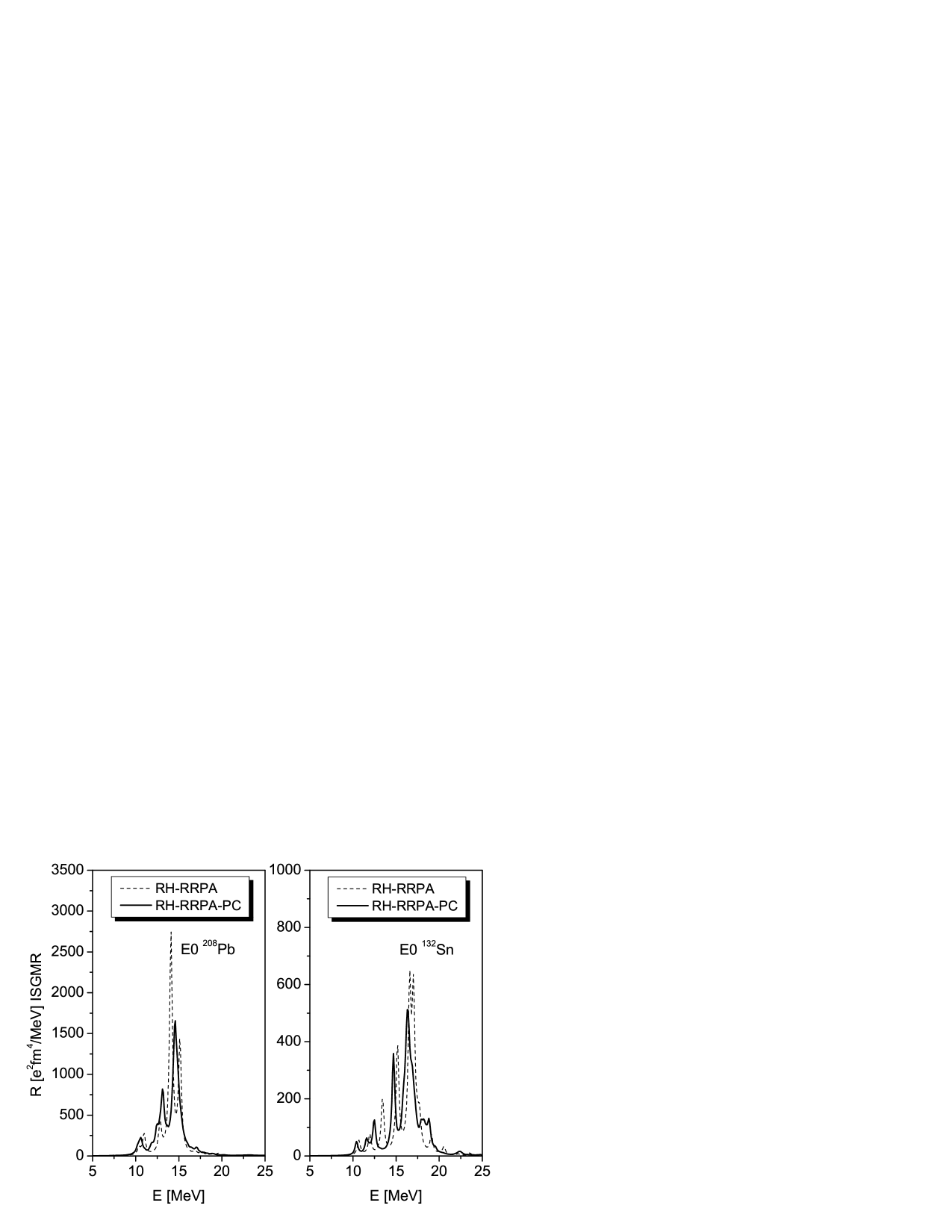
Figure 3: Isoscalar monopole resonance in ²⁰⁸Pb and ¹³²Sn obtained within two approaches: RRPA (dashed line) and RRPA with particle-phonon coupling RRPA-PC (solid line). Both computations have been performed with relativistic Hartree (RH) mean field and employ NL3 parameter set for RMF forces.

Table 1: Lorentz fit parameters of isoscalar E0 strength function in ²⁰⁸Pb and ¹³²Sn calculated within RRPA and RRPA extended by the particle-phonon coupling model (RRPA-PC) as compared to experimental data. The fit has been carried out in the interval from $B_{n}$ to roughly 20 MeV.

		$<$E$>$ (MeV)	$\Gamma$ (MeV)
	RRPA	14.16	1.71
208Pb	RRPA-PC	14.05	2.36
	Exp. SY.93	13.73(20)	2.58(20)
	RRPA	16.10	2.63
132Sn	RRPA-PC	16.01	3.09

III.4 Isoscalar monopole and isovector dipole resonances in ²⁰⁸Pb and ¹³²Sn

The calculated strength functions for the isoscalar monopole resonance in ²⁰⁸Pb and ¹³²Sn are shown in Fig. 3. The fragmentation of the resonance caused by the particle-phonon coupling is clearly demonstrated although the spreading width of the monopole resonance is not large because of a strong cancellation between the self-energy diagrams and diagrams with the phonon exchange (see Fig. 2). This fact has also been discussed in detail in Refs. BBBD.79 ; BB.81 and it is not disturbed by the subtraction procedure (51) because this cancellation takes place as well in $\Phi(\omega)$ as in $\Phi(0)$.

In order to compare the spreading of the theoretical strength distributions with experimental data we deduce mean energies $\langle E\rangle$ and widths parameters $\Gamma$ by fitting our theoretical strength distribution in a certain energy interval to a Lorentz curve in the same way as it has been done in the experimental investigations. The mean energies and the widths parameters obtained in this way are shown in the Table 1. As experimental data we display the numbers adopted in the Ref. SY.93 from the evaluation of a series of data obtained in different experiments for the isoscalar monopole resonance in ²⁰⁸Pb.

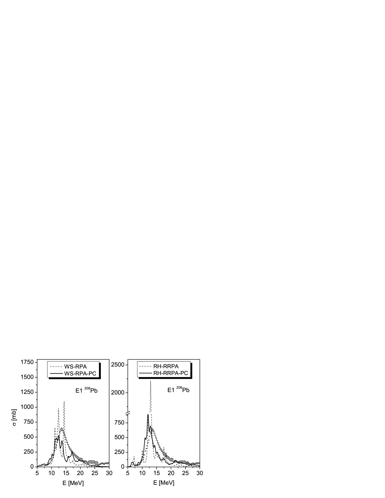
Figure 4: The isovector E1 resonance in ²⁰⁸Pb. Details are given in the text.

Figure 5: The same as in Fig. 3 but for ¹³²Sn.

Table 2: Lorentz fit parameters in the two energy intervals: $B_{n}-25$ MeV and $0-30$ MeV, for the E1 photoabsorption cross sections in ²⁰⁸Pb and ¹³²Sn, calculated with the RRPA, and with the RRPA extended to include the particle-phonon coupling (RRPA-PC), compared to data.

		$B_{n}$ - 25 MeV			0 - 30 MeV
		$<$E$>$	$\Gamma$	EWSR	$<$E$>$	$\Gamma$	EWSR
		(MeV)	(MeV)	(%)	(MeV)	(MeV)	(%)
	RRPA	13.1	2.4	121	12.9	2.0	128
208Pb	RRPA-PC	12.9	4.3	119	13.2	3.0	128
	Exp. ripl	13.4	4.1	117			125(8)
	RRPA	14.7	3.3	116	14.5	2.6	126
132Sn	RRPA-PC	14.4	4.0	112	14.6	3.2	126
	Exp. Adr.05	16.1(7)	4.7(2.1)	125(32)

The calculated photoabsorption cross sections

$$\sigma_{E1}(E)={\frac{{16\pi^{3}e^{2}}}{{9\hbar c}}}E~{}S_{E1}(E)$$ (74)

for the isovector dipole resonance in ²⁰⁸Pb and ¹³²Sn are given in the Figs. 4 and 5 respectively. The left panels show the results obtained within the non-relativistic approach with Woods-Saxon (WS) single-particle input and Landau-Migdal (LM) forces described in Ref. LT.05 . They are compared in the right panel with the relativistic fully consistent theory developed in the present work. The underlying Lagrangian has the parameter set NL3 NL3 . RPA calculations are shown by the dashed curves, RPA-PC calculations – by the thick solid curves. In Fig. 4 we have displayed experimental data with error bars taken from Ref. ripl . To make the comparison reasonable calculations within the non-relativistic framework have been performed with box boundary conditions for the Schrödinger equation in $r$-space which ensures completeness of the single-particle basis.

The corresponding Lorentz fit parameters in the two energy intervals: $B_{n}-25$ MeV and $0-30$ MeV ($B_{n}$ is the neutron separation energy) are included in Table 2 and they are compared with the data of Ref. Adr.05 ; ripl . We notice that the inclusion of particle-phonon coupling in the RRPA calculation induces a pronounced fragmentation of the photoabsorption cross sections, and brings the width of the GDR in much better agreement with the data, both for ²⁰⁸Pb and ¹³²Sn.

The fragmentation of the resonance introduced by the particle-phonon coupling is clearly demonstrated in both cases. Also, one finds more or less the same level of agreement between theory and experimental data for these two calculations. In the case of the isovector E1 resonance in ¹³²Sn this is, however, not so clear because the cross section and the integral characteristics of the resonance obtained in the experiment of Ref. Adr.05 are given with relatively large error bars. In ²⁰⁸Pb our self-consistent relativistic approach reproduces the shape of the giant dipole resonance much better than the non-relativistic one although the whole resonance is about 0.5 MeV shifted to lower energies with respect to the experiment. As one can see from the Fig. 4 and Table 2, we observe some shift already in the RRPA calculation, which is determined by the properties of the NL3 forces. Improvement of the forces, for instance, the use of the density dependent versions DD-ME1 ; DD-ME2 of the RMF should bring the E1 mean energy in better agreement with the data.

However, there is an essential difference between the fully self-consistent relativistic calculations of the present work and the non-relativistic approach: in non-relativistic approach discussed in Ref. LT.05 one introduces on all three stages of the calculation phenomenological parameters, which have to be adjusted to experimental data: first, the Woods-Saxon parameters as, for instance, the well depth are varied to obtain single-particle levels close to the experimental values, second, one of the parameters of the Landau-Migdal force is adjusted to get phonon energies at the experimental positions (for each mode) and, third, another Landau-Migdal force parameter is varied to reproduce the centroid of the giant resonance. Although the varying of the parameters is performed in relatively narrow limits, it is necessary to obtain realistic results. In contrast, in the relativistic fully consistent approach developed in the present work no adjustment of additional parameters is made. Of course, the underlying energy functional has been determined in a phenomenological way by a fit to experimental ground state properties of characteristic nuclei. However, it is of universal nature and the same parameters are used for investigations of many nuclear properties all over the periodic table. The predictive power of this scheme is therefore much higher than that of the present semi-phenomenological approach discussed, for instance, in Ref. LT.05 .

The effect of the particle-vibration coupling on the low-lying dipole strength around the neutron threshold within the presented approach can be also seen in the Figs. 4,5. But this phenomenon requires the detailed investigation and is considered in the special publication LRV.06 .

IV Summary and outlook

In order to describe the damping of collective excitations in nuclei covariant density functional theory is extended by particle-vibration coupling in a consistent way. Starting from a relativistic energy functional $E[\rho]$ the self-consistent RMF equations are solved and the static part of the nucleon self-energy $\tilde{\Sigma}=\delta E/\delta\rho$ is found. In a second step the low-lying collective phonons are determined in the framework of relativistic RPA with the effective $ph$-interaction $\tilde{V}=\delta\tilde{\Sigma}/\delta\rho$. Using particle-phonon vertices deduced from the same interaction the self-energy $\tilde{\Sigma}$ is extended by an energy dependent part $\Sigma^{e}(\varepsilon)$. The Bethe-Salpeter equation derived from the full self-energy $\Sigma=\tilde{\Sigma}+\Sigma^{e}$ is formulated in the $ph$-basis of the Dirac eigenstates. Using the time blocking approximation, which allows the truncation to $1p1h\otimes$phonon  configurations and a subtraction procedure, which avoids double counting of correlations it is shown that the resulting effective interaction $\tilde{V}+\delta\Phi(\omega)$ contains besides the static part $\tilde{V}$ an energy dependent correction term $\delta\Phi(\omega)$, which takes into account the coupling of the particles to collective phonons.

This method is applied to the computation of spectroscopic characteristics of nuclear excited states in a wide energy range up to 30 MeV for spherical nuclei with closed shells. An equation for the density matrix variation is formulated and solved in the Dirac space as well in the momentum space. The particle-phonon coupling amplitudes of collective vibrational modes below the neutron separation energy have been calculated within the self-consistent RRPA using the parameter set NL3 for the Lagrangian. The same force has been used for the static part of the effective $ph$-interaction $\tilde{V}$ and for the evaluation of the particle-phonon vertices $\gamma_{kk^{\prime}}^{\mu}$. Therefore a fully consistent description of giant resonances is performed.

Noticeable fragmentation of the isoscalar monopole and isovector dipole giant resonances in ²⁰⁸Pb and ¹³²Sn is obtained due to the particle-vibration coupling. This leads to a significant spreading width as compared to simple RRPA calculations. This is in agreement with experimental data as well as with the results obtained within the non-relativistic semi-phenomenological approaches of Refs. LT.05 ; SBC.04 .

Thus in the present work a description of nuclear many-body dynamics including complex configurations is realized within an approach which is (i) fully consistent, (ii) based on relativistic dynamics, (iii) universally valid for nuclei all over the periodic table, and (iv) based on a modern covariant density functional, which has been applied with great success for many nuclear properties all over the periodic table.

So far, this extended density functional theory for complex configurations has been formulated only for closed shell nuclei. To expand the field of applications to nuclei with opened shells it is, of course, necessary to include pairing correlations into the approach discussed in the present paper. This can be done in the manner of Ref. Tse.05 where pairing correlations and particle-vibration coupling are taken into account on an equal footing in a non-relativistic framework using techniques of a generalized Green’s function formalism. Work on this direction is in progress.

ACKNOWLEDGEMENTS

Helpful discussions with Prof. D. Vretenar are gratefully acknowledged. This work has been supported in part by the Bundesministerium für Bildung und Forschung under project 06 MT 246. E. L. acknowledges the support from the Alexander von Humboldt-Stiftung and the assistance and hospitality provided by the Physics Department of TU-München. V. T. acknowledges financial support from the Deutsche Forschungsgemeinschaft under the grant No. 436 RUS 113/806/0-1 and from the Russian Foundation for Basic Research under the grant No. 05-02-04005-DFG_a.

Appendix A Non-linear meson potentials

So far we started from a Lagrangian (1) containing the nucleons as Dirac particles and mesons providing an interaction between them Wal.74 ; SW.86 , as it is the starting point of most of the relativistic investigations in nuclear physics. It has been recognized, however, very early BB.77 that this model does not provide an adequate description of the surface properties of realistic nuclei. The incompressibility is too high and the deformations are too small GRT.90 . Therefore over the years the relativistic models have been considerably improved by introducing an effective density dependence, as it is in accordance with the concept of density functional theory. Boguta and Bodmer proposed already in 1977 to introduce a non-linear coupling between the $\sigma$-mesons replacing  the mass term $\frac{1}{2}m_{\sigma}^{2}\sigma^{2}$ in the Lagrangian (1) by a non-linear meson potential BB.77

$$U(\sigma)=\frac{1}{2}m_{\sigma}^{2}\sigma^{2}+\frac{g_{2}}{3}\sigma^{3}+\frac{g_{3}}{4}\sigma^{4}\;.$$ (75)

This procedure was used because it did not destroy the renormalizability of the model. In these early days relativistic models of the nucleus were considered as fully fledged quantum field theories SW.86 and therefore non-linear meson couplings provided an elegant extension of the model containing additional parameters introducing an effective density dependence.

In fact, models with non-linear meson couplings have been used very extensively in the literature. Very successful parameterizations have been developed on this basis as, for instance, NL1 NL1 and NL3 NL3 , which contain only non-linear couplings between the $\sigma$-mesons. Later on one also considered non-linear couplings between the $\omega$-mesons Bod.91 ; TM1 , however without improving the agreement between theoretical results and experimental data in finite nuclei. In the present investigations we consider the parameter set NL3, which has been used with great success for the description of symmetric nuclear matter and finite nuclei with closed shells GRT.90 , deformed nuclei, rotating nuclei ARK.00 and for relativistic RPA calculations of giant resonances and low-lying states MWG.02 . In the most successful applications pairing correlations are taken into account in the framework of relativistic Hartree-Bogoliubov (RHB) theory with Gogny type interactions in the pp-channel RHB . For a recent review see Ref. VALR.05 .

The effective interaction entering the static part of the nucleon self-energy is in this case given by meson exchange potentials. Without the non-linear couplings these interactions are of Yukawa type with a range determined by the mass of the corresponding mesons and with a relativistic structure determined by the quantum numbers of the mesons. In the simplest case of the $\sigma\omega$-model we have

$$\tilde{V}(1,2)=-g_{\sigma}^{2}D_{\sigma}(\bm{r}_{1},\bm{r}_{2})\beta^{(1)}\beta^{(2)}+g_{\omega}^{2}D_{\omega}(\bm{r}_{1},\bm{r}_{2})(1^{(1)}1^{(2)}-{\mbox{\boldmath$\alpha$}}^{(1)}{\mbox{\boldmath$\alpha$}}^{(2)})$$ (76)

with the Dirac matrices $\beta$ and $\bm{\alpha}$ and with the propagator in $r$-space

$$D_{m}(\bm{r}_{1},\bm{r}_{2})=\frac{1}{4\pi}\frac{e^{-m_{m}|\bm{r}_{1}-\bm{r}_{2}|}}{|\bm{r}_{1}-\bm{r}_{2}|},\text{ \ \ \ \ \ \ \ \ for \ \ }m=\sigma,\omega.$$ (77)

More realistic applications contain in addition a $\rho$-meson and the photon. These potentials are obtained from the Klein-Gordon equations by elimination of the meson degrees of freedom neglecting retardation.

In the non-linear case the static Klein-Gordon equation for the $\sigma$-meson has the form

$$-\Delta\sigma+U^{\prime}(\sigma)=-g_{\sigma}\left\langle\bar{\psi}\psi\right\rangle,$$ (78)

with

$$U^{\prime}(\sigma)=m_{\sigma}^{2}\sigma+g_{2}\sigma^{2}+g_{3}\sigma^{3}.$$ (79)

This is a nonlinear equation, which does not allow for an analytic solution. The numerical solution of Eq. (78) $\sigma(\bm{r})$ provides us with the mean field of scalar type

$$\tilde{\Sigma}_{s}(\bm{r})=g_{\sigma}\sigma(\bm{r)}.$$ (80)

Relativistic RPA is obtained as the small amplitude limit of time-dependent Hartree theory RMG.01 . In this case the relativistic single-particle density matrix $\rho_{kk^{\prime}}$ is expanded around the static solution $\rho_{0}$. The linearization of the Klein-Gordon equation (78) leads to

$$(-\Delta+M(\bm{r}))\delta\sigma=-g_{\sigma}{\delta\rho}_{s},$$ (81)

where ${\delta\rho}_{s}$ is the scalar density, with $M(\bm{r})$ depending on the coordinate $\bm{r}$

$$M(\bm{r})=U^{\prime\prime}(\sigma_{0}(\bm{r}))=m_{\sigma}^{2}+2g_{2}\sigma_{0}(\bm{r})+3g_{3}\sigma_{0}^{2}(\bm{r}).$$ (82)

where $\sigma_{0}(\bm{r})$ is the $\sigma$-field of the static solutions. In momentum space this leads to a non-local propagator, which is the solution of the integral equation

$$\bm{q}^{2}D_{\sigma}(\bm{q},\bm{q}^{\prime})+{\displaystyle\int}\frac{d^{3}q^{\prime\prime}}{(2\pi)^{3}}~{}M(\bm{q-q}^{\prime\prime})D_{\sigma}(\bm{q}^{\prime\prime},\bm{q}^{\prime})=(2\pi)^{3}\delta(\bm{q}-\bm{q}^{\prime}),$$ (83)

where $M(\bm{q})$ is the Fourier transform of $M(\bm{r})$:

$$M(\bm{q})={\displaystyle\int}d^{3}re^{-i\bm{qr}}M(\bm{r)}.$$ (84)

The $\sigma$ part of the effective ph-interaction used in the RPA calculations has therefore the form

$$\tilde{V}_{\sigma}^{ph}(1,2)=-g_{\sigma}^{2}\beta^{(1)}\beta^{(2)}{\displaystyle\int}\frac{d^{3}qd^{3}q^{\prime}}{(2\pi)^{6}}\ e^{i(\bm{qr}_{1}\bm{-q}^{\prime}\bm{r}_{2})}D_{\sigma}(\bm{q},\bm{q}^{\prime})$$ (85)

and similar terms for the other mesons and the photon. We use this interaction in the solution of the relativistic RPA equation for the calculation of the collective phonons, as well as in Eq. (19) for the determination of the corresponding particle-phonon vertices $\gamma_{kl}^{\mu}$  and in Eq. (36) for the response function $R(14,23)$.

Appendix B Density dependent meson vertices

In recent years it has been recognized that the relativistic models are by no means fully fledged quantum field theories. Instead of that they are effective field theories, which provide the basis of covariant density functional theory. Renormalizability is not important. In the spirit of density functional theory it is reasonable to abandon the non-linear couplings and to introduce instead of that coupling parameters $g_{\sigma}(\rho(\bm{r}))$, $g_{\omega}(\rho(\bm{r)})$ and $g_{\rho}(\rho(\bm{r)})$, which depend on the baryon density BT.92 ; FL.95 ; FLW.95 ; TW.99 ; DD-ME1 ; DD-ME2 .

In this case the static self-energy contains rearrangement terms, i.e. terms depending on the derivative of the coupling constant with respect to the density. We find

$$\tilde{\Sigma}_{s}(\bm{r}) =g_{\sigma}\sigma(\bm{r)}$$ (86)

$$\tilde{\Sigma}_{0}(\bm{r}) =g_{\omega}\omega_{0}(\bm{r)+}g_{\rho}\tau_{3}\rho_{0}(\bm{r)+}V_{C}(\bm{r)+}\text{ }\tilde{\Sigma}^{R}(\bm{r})$$ (87)

with the rearrangement term

$$\text{ }\tilde{\Sigma}^{R}(\bm{r})=g_{\sigma}^{\prime}(\rho(\bm{r))}\rho_{s}(\bm{r)}\sigma(\bm{r)}+g_{\omega}^{\prime}(\rho(\bm{r))}\rho(\bm{r)}\omega_{0}(\bm{r)}+g_{\rho}^{\prime}(\rho(\bm{r))}\rho_{T}(\bm{r)}\rho_{0}(\bm{r)},$$ (88)

where $\rho=\rho_{p}+\rho_{n}$ and $\rho_{T}=\rho_{p}-\rho_{n}$ are the isoscalar and isovector baryon densities and where $\rho_{0}$ is the time-like component of the $\rho$-field. Here we have used the fact, that we have time-reversal invariance in the ground state and that the currents vanish in this case.

The effective ph-interaction is obtained as the derivative of the self-energy with respect to the density operator. We find for the $\sigma$-exchange

$$V_{\sigma}^{ph}(1,2) =-\beta^{(1)}\beta^{(2)}g_{\sigma}(1)g_{\sigma}(2)D_{\sigma}(\bm{r}_{1},\bm{r}_{2})-I_{\sigma}(\bm{r}_{1})\delta(\bm{r}_{1}-\bm{r}_{2})$$

$$-\{\beta^{(1)}1^{(2)}g_{\sigma}(1)\tilde{g}_{\sigma}(2)+1^{(1)}\beta^{(2)}\tilde{g}_{\sigma}(1)g_{\sigma}(2)+1^{(1)}1^{(2)}\tilde{g}_{\sigma}(1)\tilde{g}_{\sigma}(2)\}D_{\sigma}(\bm{r}_{1},\bm{r}_{2})$$ (89)

with

$$I_{\sigma}(\bm{r}_{1})=\left\{(\beta^{(1)}1^{(2)}+1^{(1)}\beta^{(2)})g_{\sigma}^{\prime}(1)+1^{(1)}1^{(2)}g_{\sigma}^{\prime\prime}(1)\rho_{s}({\bm{r}}_{1})\right\}\times$$

$$\times\int d^{3}r\ g_{\sigma}(\rho(\bm{r}))D_{\sigma}(\bm{r}_{1},\bm{r})\rho_{s}(\bm{r})$$ (90)

and similar terms for the $\omega$- and $\rho$-exchange. Here we have used the abbreviations:

$$g_{\sigma}(1) :=g_{\sigma}(\rho(\bm{r}_{1}))$$ (91)

$$\tilde{g}_{\sigma}(1) :=g_{\sigma}^{\prime}(\rho(\bm{r}_{1}))\rho_{s}(\bm{r}_{1}).$$ (92)

Appendix C Solution in momentum space

First we concentrate on the static interaction $\tilde{V}$ of Eq. (76) neglecting for the moment the non-linear meson coupling. We can transform the one-boson exchange (OBE) interaction (76) to momentum space and neglect retardation:

$$\tilde{V}(1,2)=\pm{\displaystyle\sum\limits_{m}}g_{m}^{2}\int\frac{d^{3}q}{(2\pi)^{3}}e^{i\mathbf{q(r}_{1}-\mathbf{r}_{2})}\Gamma_{\mu}^{m}(1)D_{m}^{\mu\nu}(q)\Gamma_{\nu}^{m}(2)$$ (93)

where the $+$sign holds for the vector mesons and the $-$sign for the scalar mesons. The index $m$ denotes the set of mesons $m=\{\sigma,\omega,\rho,e\}$ – the isoscalar-scalar $\sigma$-meson, the isoscalar-vector $\omega$-meson, the isovector-vector $\rho$-meson and the photon, which carry the respective components of the interaction. Summation is implied also over the repeated Greek indices. $D_{m}^{\mu\nu}(q)$ is a boson propagator which is usually taken in the RMF calculations in the simplified Yukawa form neglecting formfactors and retardation effects:

$$D_{m}(q) =-\frac{1}{\mathbf{q}^{2}+m_{m}^{2}},\ \ \ \ \ m=\sigma,$$ (94)

$$D_{m}^{\mu\nu}(q) =\frac{g^{\mu\nu}}{\mathbf{q}^{2}+m_{m}^{2}},\ \ \ \ \ m=\omega,\rho,e.$$ (95)

Introducing the channel index $c=(\mathbf{q},m)$, which combines the meson index $m$ with the momentum transfer $\mathbf{q}$, we can express $\tilde{V}$ as a sum of separable terms

$$\tilde{V}(1,2)=\sum\limits_{c}d_{c}Q^{(c)}(1)Q^{(c)\dagger}(2)$$ (96)

with

$$Q^{(c)}=Q(\mathbf{q},m)=\Gamma_{\mu}^{m}e^{i\mathbf{qr}}$$ (97)

and the propagator

$$d_{c}=d(\mathbf{q},m)=\pm g_{m}^{2}D_{m}^{\mu\nu}(q).$$ (98)

The matrix elements of $\tilde{V}$ in Dirac space have the form

$$\tilde{V}_{k_{1}k_{4},k_{2}k_{3}} =\langle k_{1}k_{4}|\tilde{V}|k_{2}k_{3}\rangle=\sum\limits_{c}d_{c}Q_{k_{1}k_{2}}^{(c)}Q_{k_{3}k_{4}}^{(c)\ast}$$

$$=\pm\sum\limits_{m}g_{m}^{2}\int\frac{d^{3}q}{(2\pi)^{3}}\langle k_{1}|\Gamma_{\mu}^{m}e^{i\mathbf{q}\mathbf{r}}|k_{2}\rangle D_{m}^{\mu\nu}(q)\langle k_{4}|\Gamma_{\nu}^{m}e^{-i\mathbf{q}\mathbf{r}}|k_{3}\rangle.$$ (99)

For non-linear meson-couplings this expression has to be somewhat modified, because the propagator in momentum space (85) is non-diagonal in this case. We have $D_{m}^{\mu\nu}(\mathbf{q},\mathbf{q}^{\prime})$ and the values $d_{c}$ have to be replaced by matrices $d_{cc^{\prime}}$ in this case.

Appendix D Response formalism in spherical nuclei

In the spherical case angular momentum coupling reduces the numerical effort considerably. The response equation for $\delta\rho$ reads in this case:

$$\delta\rho_{(k_{1}k_{2})}^{J}(\omega) ={\tilde{\delta\rho}}_{(k_{1}k_{2})}^{J}(\omega)+$$

$$+{\tilde{R}}_{(k_{1}k_{2})}(\omega)\sum\limits_{(k_{3}k_{4})}\Bigl{[}{\tilde{V}}_{(k_{1}k_{4},k_{2}k_{3})}^{J}+\delta\Phi_{(k_{1}k_{4},k_{2}k_{3})}^{J}(\omega)\Bigr{]}\delta\rho_{(k_{3}k_{4})}^{J}(\omega).$$ (100)

It contains the matrix elements of the static effective interaction $\tilde{V}^{J}$   and $\delta\Phi^{J}(\omega)$ is the change of the effective interaction due to the energy dependence of the particle-vibration coupling.

For the meson exchange potentials we obtain after coupling to good angular momentum $J$:

$$\tilde{V}_{(k_{1}k_{4},k_{2}k_{3})}^{J} =\pm\frac{(4\pi)^{2}}{2J+1}\sum\limits_{LSm}(-1)^{S}\,\int\limits_{0}^{\infty}\frac{q^{2}dq}{(2\pi)^{3}}\langle k_{1}\|j_{L}(qr)[\Gamma_{S}^{m}Y_{L}]^{J}\|k_{2}\rangle\times$$

$$\quad\quad\quad\quad\quad\quad\quad\quad\ \ \ \ \ \ \ \ \ \ \quad\quad\quad\quad\times\frac{g_{m}^{2}}{q^{2}+m_{m}^{2}}\langle k_{3}\|j_{L}(qr)[\Gamma_{S}^{m}Y_{L}]^{J}\|k_{4}\rangle,$$ (101)

where index $S=(0,1)$ denotes the spherical component of the Pauli matrix entering the vertices (3). The factor $(-)^{S}$ indicates that the space-like parts of the interaction (current-current interactions) have the opposite sign as the time-like part. The matrix elements (101) are a sum of separable terms. The dimension of the matrices to be inverted is given by the number of separable terms.

The interaction $\tilde{V}$ is treated in the response equation Eq. (72). After a transformation of this equation to momentum space we find

$$\delta\rho_{LS}^{Jm}(q,\omega) ={{\delta\rho}}_{LS}^{(e)Jm}(q;\omega)\pm\,$$

$$\pm\frac{(4\pi)^{2}}{2J+1}\sum\limits_{L^{\prime}S^{\prime}m^{\prime}}(-1)^{S^{\prime}}\int\limits_{0}^{\infty}\frac{q^{\prime\ 2}dq^{\prime}}{(2\pi)^{3}}R_{LS,L^{\prime}S^{\prime}}^{(e)Jmm^{\prime}}(q,q^{\prime};\omega)\frac{g_{m^{\prime}}^{2}}{q^{\prime\ 2}+m_{m^{\prime}}^{2}}\delta\rho_{L^{\prime}S^{\prime}}^{Jm^{\prime}}(q^{\prime};\omega),$$ (102)

where

$$R_{LS,L^{\prime}S^{\prime}}^{(e)Jmm^{\prime}}(q,q^{\prime};\omega)=\sum\limits_{(k_{1}k_{2}k_{3}k_{4})}Q_{LS(k_{1}k_{2})}^{Jm}(q)R_{(k_{1}k_{4},k_{2}k_{3})}^{(e)J}(\omega)Q_{L^{\prime}S^{\prime}(k_{3}k_{4})}^{Jm^{\prime}}(q^{\prime})$$ (103)

with

$$Q_{LS(k_{1}k_{2})}^{Jm}(q)=\langle k_{1}\|j_{L}(qr)[\Gamma_{S}^{m}Y_{L}]^{J}\|k_{2}\rangle$$ (104)

is a Fourier transform of the correlated propagator $R^{(e)J}$ which is determined in the Dirac basis by the angular momentum coupled version of Eq. (66) :

$$R_{(k_{1}k_{4},k_{2}k_{3})}^{(e)J}(\omega)={\tilde{R}}_{(k_{1}k_{2})}(\omega)\delta_{(k_{1}k_{3})}\delta_{(k_{2}k_{4})}\,+{\tilde{R}}_{(k_{1}k_{2})}(\omega)\sum\limits_{(k_{5}k_{6})}\delta\Phi_{(k_{1}k_{6},k_{2}k_{5})}^{J}(\omega)R_{(k_{5}k_{4},k_{6}k_{3})}^{(e)J}(\omega).$$ (105)

The free term on the right side of the Eq. (102) has the following form:

$${{\delta\rho}}_{LS}^{(e)Jm}(q;\omega)=\sum\limits_{(k_{1}k_{2}k_{3}k_{4})}Q_{LS(k_{1}k_{2})}^{Jm}(q)R_{(k_{1}k_{4},k_{2}k_{3})}^{(e)}(\omega)P_{(k_{3}k_{4})}^{J},$$ (106)

where

$$P_{(k_{1}k_{2})}^{J}=\langle k_{1}\|P^{J}\|k_{2}\rangle.$$ (107)

The spectrum of nuclear excitations in the external field $P$ with the multipolarity $J$ is therefore determined by the strength function:

$$S^{J}(E)=-\frac{1}{\pi}\lim\limits_{\Delta\rightarrow+0}Im\ \Pi^{J}(E+i\Delta),$$ (108)

expressed through the following polarizability $\Pi^{J}(\omega)$:

$$\Pi^{J}(\omega)=\Pi^{(e)J}(\omega)\pm\frac{(4\pi)^{2}}{2J+1}\sum\limits_{LSm}(-1)^{S}\int\limits_{0}^{\infty}\frac{dqq^{2}}{(2\pi)^{3}}{\delta\rho}_{LS}^{(e)Jm}(q;\omega)\frac{g_{m}^{2}}{q^{2}+m_{m}^{2}}\delta\rho_{LS}^{Jm}(q;\omega),$$ (109)

where

$$\Pi^{(e)J}(\omega)=\sum\limits_{(k_{1}k_{2}k_{3}k_{4})}P_{(k_{1}k_{2})}^{J}R_{(k_{1}k_{4},k_{2}k_{3})}^{(e)J}(\omega)P_{(k_{3}k_{4})}^{J}.$$ (110)

Thus, one can see that it is convenient to solve our problem as well as the RRPA problem in the momentum space since the rank of vectors and matrices entering the Eq. (102) is determined by the number of mesh points in $q$-space and the number of meson channels. In particular it does not depend on the mass number of the nucleus. In realistic calculations the rank of the Eq. (102) in the momentum space is around 500 and, obviously, the numerical effort does not depend considerably on the total dimension of $ph$ and $\alpha h$ subspaces. However, if one stays in the Dirac basis the latter dimension is exactly the rank of arrays in the Eq. (100). One should keep in mind that in practice both subspaces are truncated at some energy differences $\varepsilon_{ph}$ and $\varepsilon_{\alpha h}$ which are large enough so that a further increase of these values does not influence the results. In light nuclei with relatively small level density the total dimension of $ph$ and $\alpha h$ subspaces is comparable and could be even smaller than the rank of the Eq. (102) and, therefore, working in the Dirac basis is more preferable. For heavy nuclei the Dirac basis becomes huge and, therefore, using of the momentum space is more justified.

However, even if one considers the Eq. (102) in the momentum representation, Eq. (105) for the correlated propagator, nevertheless, has to be solved in the Dirac basis. This equation contains the particle-phonon coupling amplitude $\Phi^{J}$ with the following matrix elements coupled to angular momentum $J$:

$$\Phi_{(ph^{\prime},hp^{\prime})}^{J}(\omega) =\sum\limits_{\mu}\Bigl{[}\delta_{(pp^{\prime})}\frac{\delta_{{\varkappa}_{h^{\prime}}{\varkappa}_{h}}}{2j_{h}+1}\sum\limits_{h^{\prime\prime}}\frac{\gamma_{(h^{\prime\prime}h)}^{\mu}\gamma_{(h^{\prime\prime}h^{\prime})}^{\mu\ast}}{\omega-\varepsilon_{p}+\varepsilon_{h^{\prime\prime}}-\Omega^{\mu}}$$

$$+\delta_{(hh^{\prime})}\frac{\delta_{{\varkappa}_{p^{\prime}}{\varkappa}_{p}}}{2j_{p}+1}\Bigl{(}\sum\limits_{p^{\prime\prime}}\frac{\gamma_{(pp^{\prime\prime})}^{\mu}\gamma_{(p^{\prime}p^{\prime\prime})}^{\mu\ast}}{\omega-\varepsilon_{p^{\prime\prime}}+\varepsilon_{h}-\Omega^{\mu}}+\sum\limits_{{\alpha}^{\prime\prime}}\frac{\gamma_{(p{\alpha}^{\prime\prime})}^{\mu}\gamma_{(p^{\prime}{\alpha}^{\prime\prime})}^{\mu\ast}}{\omega-\varepsilon_{{\alpha}^{\prime\prime}}+\varepsilon_{h}-\Omega^{\mu}}\Bigr{)}$$

$$+(-1)^{J+J_{\mu}}\left\{\begin{array}[c]{ccc}j_{p}&j_{h}&J\\ j_{h^{\prime}}&j_{p^{\prime}}&J^{\mu}\end{array}\right\}\Bigl{(}\frac{(-1)^{j_{p^{\prime}}-j_{h}}\gamma_{(pp^{\prime})}^{\mu}\gamma_{(hh^{\prime})}^{\mu\ast}}{\omega-\varepsilon_{p^{\prime}}+\varepsilon_{h}-\Omega^{\mu}}+\frac{(-1)^{j_{p}-j_{h^{\prime}}}\gamma_{(p^{\prime}p)}^{\mu\ast}\gamma_{(h^{\prime}h)}^{\mu}}{\omega-\varepsilon_{p}+\varepsilon_{h^{\prime}}-\Omega^{\mu}}\Bigr{)}\Bigr{]},$$ (113)

where $\varkappa_{k}$ denotes the relativistic quantum number set: $\varkappa_{k}=(2j_{k}+1)(l_{k}-j_{k})$, and $\gamma_{(k_{1}k_{2})}^{\mu}=\langle k_{1}\|\gamma^{\mu}\|k_{2}\rangle$ denotes the reduced matrix element of the particle-phonon coupling amplitude. The backwards going components are found through the symmetry relations:

$$\Phi_{(hp^{\prime},ph^{\prime})}^{J}(\omega)=(-1)^{j_{h}+j_{p}+j_{h^{\prime}}+j_{p^{\prime}}}\Phi_{(p^{\prime}h,h^{\prime}p)}^{J}(-\omega).$$ (114)

But this problem is too expensive numerically to be solved in the full Dirac basis. Due to the pole structure of the $\Phi$ amplitude it is naturally to suggest that particle-phonon coupling effect is not important quantitatively far from the Fermi surface. So, in the numerical calculations an energy window $\varepsilon_{win}$ was implied around the Fermi surface with respect to $ph$ energy differences $\varepsilon_{ph}$ so that the summation in the Eq. (105) is performed only among the $ph$ pairs with $\varepsilon_{ph}\leq\varepsilon_{win}$. Consequently, the correlated propagator differs from the mean field propagator only within this window. This approximation has been investigated numerically by direct calculations with different values of $\varepsilon_{win}$ as it is discussed in Sec. III. It is important to emphasize that many $ph$ and $\alpha h$ configurations outside of the window are taken into account on the RRPA level that is necessary in order to obtain the reasonable centroid positions of giant resonances as well as to find the dipole spurious state close to zero energy.

REFERENCES

REFERENCES

- (1) P. Hohenberg and W. Kohn, Phys. Rev. 136, B864 (1964).
- (2) W. Kohn and L. J. Sham, Phys. Rev. 137, A1697 (1965).
- (3) D. Vautherin and D. M. Brink, Phys. Rev. C5, 626 (1972).
- (4) J. Dechargé and D. Gogny, Phys.Rev. C21, 1568 (1980).
- (5) P. Ring, Prog. Part. Nucl. Phys. 37, 193 (1996).
- (6) D. Vretenar, A. V. Afanasjev, G. A. Lalazissis, and P. Ring, Phys. Rep. 409, 101 (2005).
- (7) Y. K. Gambhir, P. Ring, and A. Thimet, Ann. Phys. (N.Y.) 198, 132 (1990).
- (8) G. Lalazissis, D. Vretenar, and P. Ring, Eur. Phys. J. A22, 37 (2004).
- (9) G. A. Lalazissis, M. M. Sharma, P. Ring, and Y. K. Gambhir, Nucl. Phys. A608, 202 (1996).
- (10) T. Bürvenich, M. Bender, J. A. Maruhn, and P.-G. Reinhard, Phys. Rev. C69, 014307 (2004).
- (11) J. Meng and P. Ring, Phys. Rev. Lett. 77, 3963 (1996).
- (12) G. A. Lalazissis, D. Vretenar, and P. Ring, Phys. Rev. C69, 017301 (2004).
- (13) G. A. Lalazissis, D. Vretenar, and P. Ring, Nucl. Phys. A650, 133 (1999).
- (14) W. Koepf and P. Ring, Nucl. Phys. A493, 61 (1989).
- (15) A. V. Afanasjev, P. Ring, and J. König, Nucl. Phys. A676, 196 (2000).
- (16) P. Ring, Z.-Y. Ma, N. Van Giai, D. Vretenar, A. Wandelt, and L.-G. Cao, Nucl. Phys. A694, 249 (2001).
- (17) N. Paar, P. Ring, T. Nikšić, and D. Vretenar, Phys. Rev. C67, 034312 (2003).
- (18) N. Paar, T. Nikšić, D. Vretenar, and P. Ring, Phys. Rev. C69, 054303 (2004).
- (19) A. Ansari, Phys. Lett. B623, 37 (2005).
- (20) T. Nikšić, D. Vretenar, and P. Ring, Phys. Rev. C73, 034308 (2006); C74, 064309 (2006).
- (21) L. D. Landau, Sov. Phys. JETP 8, 70 (1959).
- (22) A. B. Migdal, Theory of Finite Fermi Systems: Applications to Atomic Nuclei (Wilson Interscience, New York, 1967).
- (23) P. Ring and J. Speth, Nucl. Phys. A235, 315 (1974).
- (24) P. Ring and E. Werner, Nucl. Phys. A211, 198 (1973).
- (25) I. Hamamoto and P. J. Siemens, Nucl. Phys. A269, 199 (1976).
- (26) A. Bohr and B. Mottelson, Nuclear Structure, Vol. 2 (Benjamin, New York, 1975).
- (27) P. F. Bortignon, R. A. Broglia, D. R. Bes, and R. J. Liotta, Phys. Rep. 30C, 305 (1977).
- (28) P. F. Bortignon, R. A. Broglia, D. R. Bes, and C. M. Dasso, Phys. Rep. 120, 1 (1985).
- (29) G.F. Bertsch, P.F. Bortignon, R.A. Broglia, and C.H. Dasso, Phys. Lett. 80B, 161 (1979).
- (30) P.F. Bortignon and R.A. Broglia, Nucl. Phys. A371, 405 (1981).
- (31) G. Colò, P.F. Bortignon, Nguyen Van Giai, A. Bracco, and R.A. Broglia, Phys. Lett. 276B, 279 (1992).
- (32) G. Colò and P.F. Bortignon, Nucl. Phys. A696, 427 (2001).
- (33) D. Sarchi, P.F. Bortignon, and G. Colo, Phys. Lett. B601, 27 (2004).
- (34) V.I. Tselyaev, Yad. Fiz. 50, 1252 (1989) [Sov. J. Nucl. Phys. 50, 780 (1989)].
- (35) S.P. Kamerdzhiev, G.Ya. Tertychny, and V.I. Tselyaev, Phys. Part. Nucl. 28, 134 (1997).
- (36) S. P. Kamerdzhiev, J. Speth, and G. Tertychny, Phys. Rep. 393, 1 (2004).
- (37) V.I. Tselyaev, Phys. Rev. C75, 024306 (2007).
- (38) E.V. Litvinova and V.I. Tselyaev, arXiv:nucl-th/0512030.
- (39) V.G. Soloviev, Theory of Atomic Nuclei: Quasiparticles and Phonons (Institute of Physics, Bristol and Philadelphia, USA, 1992).
- (40) S. Drożdż, S. Nishizaki, J. Speth, and J. Wambach, Phys. Rep. 197, 1 (1990).
- (41) V. A. Khodel and E. E. Saperstein, Nucl. Phys. A317, 424 (1979).
- (42) V. A. Khodel and E. E. Saperstein, Nucl. Phys. A348, 261 (1980).
- (43) S. A. Fayans, S. V. Tolokonnikov, E. L. Trykov, and D. Zawischa, Nucl. Phys. A676, 49 (2000).
- (44) E. Litvinova and P. Ring, Phys. Rev. C73, 044328 (2006).
- (45) G. A. Lalazissis, J. König, and P. Ring, Phys. Rev. C55, 540 (1997).
- (46) J.D. Walecka, Ann. Phys. 83, 491 (1974).
- (47) B.B. Serot and J.D. Walecka, Adv. Nucl. Phys. 16, 1 (1986).
- (48) S. Shlomo and D.H. Youngblood, Phys. Rev. C47, 529 (1993).
- (49) P. Adrich, A. Klimkewicz, M. Fallot et al., Phys. Rev. Lett. 95, 132501 (2005).
- (50) A. Veyssiere, H. Beil, R. Bergere, P. Carlos, and A. Lepretre, Nucl. Phys. A159, 561 (1970).
- (51) T. Nikšić, D. Vretenar, P. Finelli, and P. Ring, Phys. Rev. C66, 024306 (2002).
- (52) G. A. Lalazissis, T. Nikšić, D. Vretenar, and P. Ring, Phys. Rev. C71, 024312 (2005).
- (53) E. Litvinova, P. Ring, and D. Vretenar, Phys. Lett. B647, 111 (2007).
- (54) J. Boguta and A. R. Bodmer, Nucl. Phys. A292, 413 (1977).
- (55) P.G. Reinhard, M. Rufa, J. Maruhn, W. Greiner, and J. Friedrich, Z. Phys. A323, 13 (1986).
- (56) A.R. Bodmer, Nucl. Phys. A526, 703 (1991).
- (57) Y. Sugahara and H. Toki, Nucl. Phys. A579, 557 (1994).
- (58) Z.-Y. Ma, A. Wandelt, N. Van Giai, D. Vretenar, P. Ring, and L.-G. Cao, Nucl. Phys. A703, 222 (2002).
- (59) P. Ring and P. Schuck, The nuclear many-body problem (Springer, Heidelberg, 1980).
- (60) T. Gonzales-Llarena, J. L. Egido, G. A. Lalazissis, and P. Ring, Phys. Lett. B379, 13 (1996).
- (61) R. Brockmann and H. Toki, Phys. Rev. Lett. 68, 3408 (1992).
- (62) C. Fuchs and H. Lenske, Phys. Lett. B345, 355 (1995).
- (63) C. Fuchs, H. Lenske, and H. H. Wolter, Phys. Rev. C52, 3043 (1995).
- (64) S. Typel and H. H. Wolter, Nucl. Phys. A656, 331 (1999).