Anisotropic probabilistic cellular automaton for a predator-prey system

Abstract

We consider a probabilistic cellular automaton to analyze the stochastic dynamics of a predator-prey system. The local rules are Markovian and are based in the Lotka-Volterra model. The individuals of each species reside on the sites of a lattice and interact with an unsymmetrical neighborhood. We look for the effect of the space anisotropy in the characterization of the oscillations of the species population densities. Our study of the probabilistic cellular automaton is based on simple and pair mean-field approximations and explicitly takes into account spatial anisotropy.

1  Introduction

In the last years a particular great effort has been done in order to understand the role of space given by a spatial structure and local interactions in the characterization of the dynamics of competing biological species systems [1, 2, 3, 4, 5, 6, 7, 8, 9, 10, 11, 12, 13, 14, 15, 16, 17, 18]. In this context it has been studied irreversible stochastic lattice models [19, 20, 21] with the purpose of mimic predator-prey systems with Markovian local rules based in the Lotka-Volterra model [22, 23]. One of the problems that has been object of study is the connection between the time oscillations of population densities and spatial pattern distribution of the individuals of each species.

Here we study the coexistence of a two-species system by considering a probabilistic cellular automaton (PCA) which is a modified version of the automaton devised in [10, 14, 17, 18]. The model, to be called anisotropic predator-prey PCA possess local rules that are similar to the ones of the cellular automaton proposed in [24]  and was introduced by us in order to explore the effect of spatial anisotropy in the temporal oscillations.

We report dynamic mean-field approximations which take into account the spatial dependence of densities and pair correlations of sites. In the next section we present the model. In Sec. 2 we show the equations for the time evolution of species densities and show the spatial dependence of these equations. In Sec. 3 and 4 we perform dynamic simple and pair mean-field approximations. Last section summarize the model, method and results.

2 Model

The physical space occupied by the species is represented by a regular lattice of $N$ sites in which each site can be in one of three states. At each site of the lattice we attach a stochastic variable $\eta_{i}$ that takes the values $0$, $1$ and $2$ according whether the site $i$ is empty, or occupied by a prey or occupied by a predator, respectively. The state of the system can be represented by the vector $\eta=(\eta_{1},\eta_{2},\ldots,\eta_{N})$. The time evolution equation for $P_{\ell}(\eta)$, the probability of state $\eta$ at time $\ell$, is given by

$$P^{\ell+1}(\eta)=\sum_{\sigma^{\prime}}W(\eta|\eta^{\prime})P^{\ell}(\eta^{\prime})$$ (1)

where the sum is over the $3^{N}$ configurations of the system and $W(\eta|\eta^{\prime})$ is the transition probability from a state $\eta^{\prime}$ to state $\eta$, given that at the previous time step the system was in state $\eta^{\prime}$. Since we are considering probabilistic cellular automata, all the sites are updated simultaneously. In this case we have

$$W(\eta|\eta^{\prime})=\prod_{i=1}^{N}w_{i}(\eta_{i}|\eta^{\prime})$$ (2)

where $w_{i}(\eta_{i}|\eta^{\prime})$ is the conditional transition probability per site.

2.1 The anisotropic predator-prey PCA

Figure 1: Transitions of the predator-prey model. The three states are: prey (1), predator (2) and empty (0). The allowed transitions obey the cyclic order shown.

The stochastic rules, embodied in the transition rate $w_{i}(\eta_{i}|\eta^{\prime})$, are set up in order that the allowed transitions between states are only the ones that obey the cyclic order shown in Fig. 1. Prey can only born in empty sites; prey can give place to a predator in a process where the prey dies and the predator is instantaneously born; finally predator can die leaving an empty site. The empty sites are places where prey can proliferate and can be seen as the resource for prey surveillance. The death of predators complete this cycle, reintegrating to the system the resources for prey.

The anisotropic predator-prey PCA has three parameters: $a$, the probability of birth of prey, $b$, the probability of birth of predator and death of prey, and $c$, the probability of predator death. Two of the process are catalytic: the occupancy of a site by prey or by a predator is conditioned, respectively, to the existence of prey or predator in the neighborhood of the site. The third reaction, where predator dies, is spontaneous, that is, it occurs, with probability $c$, independently of the neighbors of the site. We assume that $a+b+c=1$ with $0\leq a,b,c\leq 1$.

The transition probabilities of the anisotropic predator-prey PCA are described in what follows:

(a) If a site $i$ is empty, $\eta_{i}=0$, and if at north or east there is at least one prey, then it can be occupied by a prey, $\eta_{i}=1$, in the next time step, with a probability proportional to the parameter $a$ and to the number of prey $n_{a}$ at north and east of site $i$.

(b) If a site is occupied by a prey, $\eta_{i}=1$, then the site has a probability of being occupied by a new predator, $\eta_{i}=2$, in the next time step if there are prey at north or east. In this process the prey dies instantaneously. The transition probability is proportional to the parameter $b$ and the number of predators at north and east of site $i$.

(c) If site $i$ is occupied by a predator, $\eta_{i}=2$, it dies spontaneously with probability $c$.

The anisotropic cellular automaton is a variation of the automaton introduced in [10, 14, 17, 18]. Here each site of a regular square lattice interacts with its first neighbors only at two preferential directions. This anisotropic neighborhood consists of the northern and eastern neighbors of each site as shown in Fig. 2. The set of transition probabilities per site is given by

$$w_{i}(1|\eta)=\frac{a}{2}n_{1}\,\delta(\eta_{i},0)+(1-\frac{b}{2}n_{2})\delta(\eta_{i},1),$$ (3)

$$w_{i}(2|\eta)=\frac{b}{2}n_{2}\,\delta(\eta_{i},1)+(1-c)\delta(\eta_{i},2)$$ (4)

and

$$w_{i}(0|\eta)=(1-\frac{1}{2}an_{1})\,\delta(\eta_{i},0)+c\delta(\eta_{i},2)$$ (5)

where

$$n_{1}=\sum_{k}\delta(\eta_{k},1)\qquad\mathrm{and}\qquad n_{2}=\sum_{k}\delta(\eta_{k},2)$$ (6)

and the sum is over the neighbor sites localized at east and north of site $i$ and correspond to the number of neighbors of site $i$ occupied by prey individuals and predators individuals, respectively.

Figure 2: A site (C) of the square lattice and its two nearest neighbor sites to the east (E) and to the north (N). The layers, $n$, $n+1$, $n+2$, … are perpendicular to the southwest-northeast direction.

We have considered this probabilistic cellular automaton with the purpose of verifying the effect of anisotropy in the properties of the time oscillations of the predator-prey system. The rules considered are in some sense inspired in the north-east-center (NEC) cellular automaton [24], which also consider an unsymmetrical neighborhood of northern and eastern sites.

The present stochastic dynamics predicts the existence of states, called absorbing states, in which the system becomes trapped. Once the system has entered such a state it cannot escape from it anymore remaining there forever. There are two absorbing states. One of them is the empty lattice. The other absorbing state is the one in which the lattice is full of prey. This situation occurs if there are few predators and they become extinct. The remaining prey will then reproduce without predation filling up the whole lattice. The existence of absorbing stationary states is an evidence of the irreversible character of the model or, in other words, of the lack of detailed balance [21]. However, the most interesting states, the ones that we are concerned with in the present study, are the active states characterized by the coexistence of prey and predators.

2.2 Evolution equation for state functions

The densities of prey, predator and empty sites are defined as

$$P_{i}^{\ell}(1)=\langle\delta(\eta_{i},1)\rangle_{\ell},$$ (7)

$$P_{i}^{\ell}(2)=\langle\delta(\eta_{i},2)\rangle_{\ell},$$ (8)

$$P_{i}^{\ell}(0)=\langle\delta(\eta_{i},0)\rangle_{\ell},$$ (9)

respectively. The lower index $i$ is used to denote the site and the upper index $\ell$ stands for the time. The pair correlation of two neighbor sites $i$ and $j$ one being occupied by prey and the other by predator is defined as

$$P_{ij}^{\ell}(\begin{array}[]{cc}1&2\end{array})=\langle\delta(\eta_{i},1)\delta(\eta_{j},2)\rangle_{\ell}.$$ (10)

In this definition the sites $i$ and $j$ are two neighboring horizontal sites, the site $j$ being at the east of $i$. For two neighboring sites placed vertically we use the notation

$$P_{ik}^{\ell}\left(\begin{array}[]{c}2\\ 1\end{array}\right)=\langle\delta(\eta_{i},1)\delta(\eta_{j},2)\rangle_{\ell},$$ (11)

where $k$ denotes the neighbor of $i$ to the north.

The evolution equation for the densities can be obtained by using the rules of the automaton and the evolution equation for the probability $P^{\ell}(\eta)$. Using equations (2), (3), (4) and (5), we obtain the time evolution equation for the density of prey at site $i$,

$$P_{i}^{\prime}(1)=\frac{a}{2}\left[P_{ij}\left(\begin{array}[]{c}1\\ 0\end{array}\right)+P_{ik}(\begin{array}[]{cc}0&1\end{array})\right]+P_{i}(1)-\frac{b}{2}\left[P_{ij}\left(\begin{array}[]{c}2\\ 1\end{array}\right)+P_{ik}(\begin{array}[]{cc}1&2\end{array})\right],$$ (12)

where we have used prime and unprimed to denote quantities at time $\ell+1$ and $\ell$, respectively. Again, $P_{ij}(\begin{array}[]{c}1\\ 0\end{array})$ denotes a pair correlation of a site $i$ which is empty and its neighbor at the north $j$ which is occupied by a prey and $P_{ik}(\begin{array}[]{cc}0&1\end{array})$ denotes the pair correlation of the site $i$ which is is empty and its neighbor to the east $k$ which is occupied by a prey. Note that site $i$ is the site to be updated. The time evolution equation for the density of predators at site $i$ is given by

$$P_{i}^{\prime}(2)=\frac{b}{2}\left[P_{ij}\left(\begin{array}[]{c}2\\ 1\end{array}\right)+P_{ik}(\begin{array}[]{cc}1&2\end{array})\right]+(1-c)P_{i}(2).$$ (13)

The evolution equations for correlations of two neighbor sites are given by equations which involves clusters of two, three and four neighbors to the north and east and they are too cumbersome. We will write them in the pair approximation in the next subsection.

We will assume in the present analysis that the densities and the pair correlations are homogeneous so that the correlations of sites placed horizontally or vertically are the same. In other words the systems exhibits a specular symmetry along the southwest-northeast line (see Fig. 2). Therefore,

$$P_{ij}^{\ell}\left(\begin{array}[]{c}1\\ 0\end{array}\right)=P_{ik}^{\ell}(\begin{array}[]{cc}0&1\end{array})$$ (14)

and

$$P_{ij}^{\ell}\left(\begin{array}[]{c}2\\ 1\end{array}\right)=P_{ik}^{\ell}(\begin{array}[]{cc}1&2\end{array}).$$ (15)

3 Simple mean-field approximation

We will first analyze the equations (12) and (13) for the densities of prey and predators by means of a simple mean field approximation [21, 26, 27]. In this approximation we write the probability of a given cluster of sites as the product of the probabilities of each site. In our analysis we maintain the space dependence of each probability. This is necessary since the rules that define the model are not isotropic. We will use the notations

$$x_{n}=P_{n}(1),\qquad y_{n}=P_{n}(2)\qquad z_{n}=P_{n}(0).$$ (16)

where the index $n$ stands for a site at the $n$ layer. A layer is defined as the sites belonging to a line perpendicular to the southwest-northeast axis, as shown in Fig. 2. Using this approximation and considering equations (12) and (13) we obtain

$$x_{n}^{\prime}=az_{n}x_{n+1}+x_{n}-bx_{n}y_{n+1},$$ (17)

and

$$y_{n}^{\prime}=bx_{n}y_{n+1}+(1-c)y_{n}.$$ (18)

where $z_{n}=1-x_{n}-y_{n}$. Due to this relation there is no need for the equation for the density of empty sites.

The analysis of the above set of equations show that the stable solutions are of two types: a prey absorbing state, where the all lattice is full of prey; and an active solution with prey and predators densities constant in time and space. So, we have just homogeneous and nonoscillating solutions when we treat the anisotropic PCA by means of simple mean-field approximation. At this level of mean-field approximation the space anisotropy does not play any role in determining the kind of coexistence of species.

4 Pair-mean field approximation

Now we consider the evolution equations for one-site correlations and two site (pair) correlations. The evolution equations for the pair correlations depend on clusters of three and four sites. Following the approach of the pair approximation [25, 26, 27, 28] we write the clusters of three and four sites as products of pair correlations and one-site correlations. However, we must be careful in doing this approximation because we are maintaining the spatial anisotropy dependence of the one and two site correlations. For example, the correlation of a site at layer $n$ in state $0$, a site at layer $n+1$ in state $0$ and a site at layer $n+2$ in state $1$, is written in the pair approximation as

$$P_{n,n+1,n+2}(001)=\frac{P_{n,n+1}(00)P_{n+1,n+2}(01)}{P_{n+1}(0)}.$$ (19)

There are more complex clusters that appear in the evolution equation for pair correlations. For example, the following cluster of four sites is approximated by

$$P_{n,n+1,n+2}\left(\begin{array}[]{ccc}2&&\\ 0&0&1\end{array}\right)=\frac{P_{n,n+1}(02)P_{n,n+1}(00)P_{n+1,n+2}(01)}{P_{i}(0)P_{n+1}(0)}.$$ (20)

Observe that $P_{nn+1}(10)$ and $P_{nn+1}(01)$ are two independent variables.

Now we use the notation

$$P_{n,n+1}(01)=u_{n},\qquad P_{n,n+1}(12)=v_{n},\qquad P_{n,n+1}(02)=w_{n},$$ (21)

$$P_{n,n+1}(10)=f_{n},\qquad P_{n,n+1}(21)=g_{n},\qquad P_{n,n+1}(20)=h_{n},$$ (22)

$$P_{n,n+1}(11)=r_{n},\qquad P_{n,n+1}(22)=s_{n},\qquad P_{n,n+1}(00)=q_{n}.$$ (23)

Figure 3: Spatial oscillations of prey and predator along the southwest-northeast direction.

Using the pair approximation we derive the following equations for pair correlations,

$$u_{n}^{\,\prime}=a\left(\frac{q_{n}u_{n}}{z_{n}}-a\frac{f_{n}q_{n}u_{n+1}}{z_{n}z_{n+1}}\right)+(1-\frac{a}{2})\left(u_{n}-b\frac{u_{n}v_{n+1}}{x_{n+1}}\right)$$

$$-\frac{a}{2}\left(\frac{u_{n}^{2}}{z_{n}}-b\frac{u_{n}^{2}v_{n+1}}{z_{n}x_{n+1}}\right)+ab\frac{h_{n}u_{n+1}}{z_{n+1}}$$

$$+c\left(g_{n}-b\frac{g_{n}v_{n+1}}{x_{n+1}}\right).$$ (24)

$$v_{n}^{\,\prime}=\frac{ab}{2}\left(\frac{u_{n}v_{n+1}}{x_{n}}+\frac{f_{n}u_{n}v_{n+1}}{z_{n}x_{n+1}}\right)+\frac{1}{2}a(1-c)\frac{f_{n}w_{n}}{x_{n}}$$

$$+b\left(\frac{r_{n}v_{n+1}}{x_{n+1}}-\frac{b}{2}\frac{g_{n}r_{n}v_{n+1}}{x_{n+1}^{2}}\right)$$

$$+(1-c)\left((1-\frac{b}{2})v_{n}-b\frac{v_{n+1}^{2}}{x_{n}}\right),$$ (25)

$$w_{n}^{\,\prime}=b\left((1-\frac{a}{2})\frac{u_{n}v_{n+1}}{x_{n+1}}-\frac{a}{2}\frac{u_{n}^{2}v_{n+1}}{z_{n}x_{n+1}}\right)$$

$$-a\frac{u_{n}^{2}v_{n+1}}{z_{n}x_{n+1}}+(1-c)\left(w_{n}-\frac{a}{2}\frac{u_{n}w_{n+1}}{z_{n}}\right)$$

$$+bc\frac{g_{n}v_{n+1}}{x_{n+1}}+c(1-c)s_{n},$$ (26)

$$f_{n}^{\,\prime}=a\left(\frac{u_{n}q_{n}}{z_{n}}-a\frac{u_{n}q_{n}u_{n+1}}{z_{n}z_{n+1}}\right)-\frac{ac}{2}\frac{u_{n}w_{n}}{z_{n}}$$

$$+f_{n}-a\frac{f_{n}u_{n}}{z_{n+1}}-\frac{b}{2}\left(\frac{v_{n}f_{n}}{x_{n}}-a\frac{v_{n}f_{n}u_{n+1}}{x_{n}z_{n+1}}\right)$$

$$+c\left((1-\frac{b}{2})v_{n}-\frac{b}{2}\frac{v_{n}^{2}}{x_{n}}\right).$$ (27)

$$g_{n}^{\,\prime}=\frac{ab}{2}\frac{v_{n}f_{n}u_{n+1}}{x_{n}z_{n+1}}+\frac{1}{2}b\left(\frac{v_{n}r_{n}}{x_{n}}-b\frac{v_{n}r_{n}v_{n+1}}{x_{n}x_{n+1}}\right)$$

$$+a(1-c)\frac{h_{n}u_{n+1}}{z_{n+1}}$$

$$+(1-c)\left(g_{n}-b\frac{g_{n}v_{n+1}}{x_{n+1}}\right),$$ (28)

$$h_{n}^{\,\prime}=\frac{b}{2}\left(\frac{v_{n}f_{n}}{x_{n}}-a\frac{v_{n}f_{n}u_{n+1}}{x_{n}z_{n+1}}\right)$$

$$-\frac{bc}{2}\left(v_{n}+\frac{v_{n}^{2}}{x_{n}}\right)+(1-c)\left(h_{n}-a\frac{h_{n}u_{n+1}}{z_{n+1}}\right)$$

$$+c(1-c)s_{n}.$$ (29)

The equations for the densities are

$$x_{n}^{\,\prime}=au_{n}+x_{n}-bv_{n,j},$$ (30)

and

$$y_{n}^{\,\prime}=bv_{n}+(1-c)y_{n}.$$ (31)

Therefore, we get a set of eight equations that we have iterated to find the solutions. We considered periodic boundary conditions and an initial condition where half of the lattice with a set of densities and the other half with another set of densities.

For $a=b$ and great values of $c$ the system attains a stationary state which is the absorbing prey state. Decreasing $c$ there is a transition to an active state, coexistence of species, and we found very interesting solutions which are characterized by travelling waves of the densities of each species. In Fig. 3 we show, for a particular set of the parameters $a=b$ and $c=0.05$, the prey and predators oscillations as a function of space and for a fixed instant of time. We can see that the behavior of the space oscillations are very complex and very different from a sinusoidal wave.

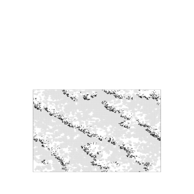
Figure 4: Snapshot of a configuration obtained from Monte Carlo simulation of the PCA in a square lattice with periodic boundary conditions. Predator and prey individual are represented by black and grey points, respectively. The fronts move from northeast to southwest.

We remark that our assumption concerning the spatial dependence of densities and pair correlations underlying our mean-field approach could not easily be conceived a priori. It was set up by considering the type of local dynamics with unsymmetrical rules and from the results of Monte Carlo simulations for the present PCA [10, 29]. To further clarify this point we show in Fig. 4 a snapshot generated by simulation of the present PCA on a square lattice where each site can be occupied by prey, predators or can be empty. Periodic boundary conditions were used and the system evolved in time according to the rules defined by Eqs. (3), (4) and (5). A synchronous update was used. We see that the distribution of individuals of each species is not homogeneous but exhibits a pattern composed by layers of prey and predators. These layers are displayed in a manner perpendicular to the southwest-northeast direction, the direction along which the oscillations occur as can be seen in Fig. 4. We have found that the spatial oscillations do not occur independently of the time oscillations, since the spatial layers of prey and predators are not static but are like fronts moving along the southwest-northeast direction. The spatial pattern oscillations are intimately associated to local time oscillations of the species [10, 29]. These features were incorporated in the present mean-field analysis of the model.

5 Conclusions

We have considered a predator-prey probabilistic cellular automaton with anisotropic local stochastic rules. We studied this model by means of dynamic mean-field approximation at two orders: simple mean-field approximation and pair mean-field approximation. Due to the anisotropy these approximations only can be performed if we consider the spatial dependence of probabilities. The simple mean-field approximation for this automaton just provides the prey absorbing state and active spatial homogeneous solutions which are also constant in time. The pair mean-field approximation gives much more rich results and show that the active states characterized by time oscillations of species densities are inhomogeneous in space. Therefore, we have spatiotemporal patterns of coexistence. This is in accordance with previous Monte Carlo simulations [10] where we have found local time oscillations connected to inhomogeneous spatial distributions of species individuals.

References

- [1] K. Tainaka, Phys. Rev. Lett. 63, 2688 (1989).
- [2] R. Durrett and S. Levin, Theor. Popul. Biol. 46, 363 (1994).
- [3] A. Hastings, Population biology: concepts and models, Springer, New York, 1997.
- [4] J. Satulovsky and T. Tomé, Phys. Rev. E bf 49, 5073 (1994).
- [5] D. Tilman and P. Kareiva, Spatial ecology: the role of space in population dynamics and interactions, Priceton University Press, Princeton, 1997.
- [6] J. Satulovsky and T. Tomé, J. Math. Biol. 35, 344 (1997).
- [7] R. Durrett and S. Levin, J. Theor. Biol. 205, 201 (2000).
- [8] T. Antal and M. Droz, Phys. Rev. E 63, 056119 (2001).
- [9] M. A. M. de Aguiar, H. Sayama, M. Baranger and Y. Bar-Yam, Braz. J. Phys. 33, 514 (2003).
- [10] K. C. de Carvalho and T. Tomé, Mod. Phys. Lett. B 18, 873 (2004).
- [11] A. F. Rozenfeld and E. V. Albano, Phys. Lett. A 332, 361 (2004).
- [12] D. Chowdhury and D. Stauffer, J. Biosc. 30, 277 (2005).
- [13] G. Szabó, J. Phys. A 38, 6689 (2005).
- [14] K. C. de Carvalho and T. Tomé, Int. J. Mod. Phys. C 17, 1647 (2006).
- [15] M. Mobilia, I T Giorgiev and U. C. Täuber, Phys. Rev. E 73, 040903 (2006).
- [16] S. Morita S and K. Tainaka, Popul. Ecol. 48, 99 (2006).
- [17] E. Arashiro and T. Tomé, J. Phys. A 40, 887 (2007)
- [18] T. Tomé and K. C. de Carvalho, Stable oscillations in a predator-prey system: a mean-field approach, arXiv:0704.0512v1 cond-mat stat-mech.
- [19] T. M. Liggett, Interacting Particle Systems, Springer, New York, 1985.
- [20] J. Marro and R. Dickman, Nonequilibrium Phase Transitions, Cambridge University Press, Cambridge, 1999.
- [21] T. Tomé and M. J. de Oliveira, Dinâmica Estocástica e Irreversibilidade, Editora da Universidade de São Paulo, São Paulo, 2001.
- [22] A. Lotka, J. Am. Chem. Soc. 42, 1595 (1920); Proc. Nat. Acad. of Sciences USA 6, 410 (1920); Elements of Mathematical Biology, Dover, New York (1924).
- [23] V. Volterra, Leçons sur la Theorie Mathématique de la Lutte pour la Vie, Gauthier-Villars, Paris, 1931.
- [24] C. H. Bennett and G. Grinstein, Phys. Rev. Lett. 55, 657 (1985).
- [25] R. Dickman, Phys. Rev. A bf 34, 4246 (1986).
- [26] T. Tomé, Physica A 212, 99 (1994).
- [27] T. Tomé and J. R. Drugowich de Felício, Phys. Rev. E 53, 3976 (1996).
- [28] T. Tomé, E. Arashiro, J. R. Drugowich de Felício and M. J. de Oliveira, Braz. J. Phys. 33, 458 (2003).
- [29] T. Tomé and K. C. de Carvalho, in preparation.