Simulation of prompt emission from GRBs with a photospheric component and its detectability by GLAST

Abstract

The prompt emission from gamma-ray bursts (GRBs) still requires a physical explanation. Studies of time-resolved GRB spectra, observed in the keV-MeV range, show that a hybrid model consisting of two components, a photospheric and a non-thermal component, in many cases fits bright, single-pulsed bursts as well as, and in some instances even better than, the Band function. With an energy coverage from 8 keV up to 300 GeV, GLAST will give us an unprecedented opportunity to further investigate the nature of the prompt emission. In particular, it will give us the possibility to determine whether a photospheric component is the determining feature of the spectrum or not. Here we present a short study of the ability of GLAST to detect such a photospheric component in the sub-MeV range for typical bursts, using simulation tools developed within the GLAST science collaboration.

1 Introduction

The Band function (see Band et al., 1993), a softly broken power-law, describes the keV-MeV spectra for a broad range of gamma-ray bursts (GRB) exceptionally well. It is an empirical function without any claim to describe the physical processes behind the continuum spectra. However, it has properties that in many bursts could be described as the result of non-thermal radiation processes, such as synchrotron or inverse Compton scattering. Some spectra, even though well-described by the Band function, can not be the result of plain optically-thin synchrotron (OTS) processes since the photon index of the sub-peak spectral slope have a value $\alpha$ larger than $-2/3$, and hence lies beyond the synchrotron ”line of death”, LOD (see Crider et al., 1997; Preece et al., 1998). Synchrotron processes may however still be a viable option through realization of synchrotron self-absorption (SSA) in a higher energy domain, see e.g. Lloyd and Petrosian (2000). The physical conditions required to produce such hard spectral slopes in the 100 keV domain are generally considered to be unreasonable but too little is known regarding the generation of magnetic fields and the relevant conditions in order to completely rule out this possibility. Inverse Compton scattering with a self-absorbed synchrotron seed spectrum residing in the optical domain (synchrotron self-Compton, SSC) is a possible mechanism for spectra with $\alpha$ larger or equal to $0$, see Panaitescu and Mészáros (2000). Still another explanation for the hard spectral slopes, suggested by Medvedev (2000), is a combination of jitter radiation and OTS radiation. Baring and Braby (2004) argued, however, that since both the latter emission processes need an almost purely non-thermal electron distribution to be able to fit the observed spectra, these emission models are difficult to reconcile with the assumed diffusive shock acceleration models, which often give rise to a strong contribution of a thermal population.

Models predicting a photospheric emission component in the prompt spectra of GRBs has been suggested by several authors (see Mészáros and Rees, 2000; Mészáros et al., 2002; Daigne and Mochkovitch, 2002; Drenkhahn and Spruit, 2002; Ryde, 2004, 2005; Rees and Mészáros, 2005; Ryde et al., 2006). Mészáros and Rees (2000) argue that the contribution of thermal radiation – originating from the expanding fireball when it becomes optically thin to Thomson scattering – could explain the hard spectral slopes in the prompt GRB spectra. Ryde shows in Ryde (2004) that some bright CGRO BATSE bursts have sub-peak spectral slopes that fit blackbody radiation very well, in agreement with results by e.g. Ghirlanda et al. (2003), and also demonstrates in Ryde (2005) that time-resolved BATSE spectra can, as an alternative to the phenomenological Band function, be fitted with a hybrid model consisting of a single power-law and a blackbody function. The hybrid model gives, for bright single pulsed bursts, just as good fit and in many cases even a better fit than the Band function. Hence, by combining a photospheric component with a power-law function, that can be interpreted as being a result of further energy dissipation in the optically thin part of the outflow, a wide range of GRBs observed by BATSE can be explained.

In this paper, we investigate the GLAST detectability of bursts containing a strong photospheric component in the sub-MeV range. A sample of 847 time-resolved spectra from 57 bright BATSE bursts were analyzed where both the Band function and the hybrid model was imposed on the data. The fits and analysis were performed with XSPEC (Arnaud and Dorman, 2003). Three representative bursts were selected for further detailed analysis and used as basis for simulations in the expanded energy range of the two instruments onboard GLAST: the GLAST Burst Monitor (GBM), covering an energy range from 8 keV to 30 MeV (hence encompassing energies both below and above the BATSE window), and the Large Area Telescope (LAT), including energies from 20 MeV up to 300 GeV. The three selected bursts, GRB911016, GRB941026 and GRB960530, were all single-pulsed, had comparable $\chi^{2}$-values and ”goodness-of-fit” ($P$-values) for both models, and showed a low-energy power-law index (Band function) that lied beyond LOD, i.e. with $\alpha$ larger than $-2/3$. The temporal features associated with each of the three bursts were extracted and the resulting data extended from the BATSE energy range (20 keV - 2 MeV) into the GLAST domain (8 keV - 300 GeV), hence assuming a strong high-energy emission. The high-energy part is generally considered to be characterized by the Band function spectral index $\beta$ that for the majority of BATSE bursts has a value less than $-2$. Of the few observed bursts that has high-energy spectra available, some do however show a strong high-energy emission González et al. (2003). In section 2 we first describe how the BATSE data was parameterized and the model that was used for the GLAST simulations. Section 3 explains how the simulated GLAST data was produced and section 3 presents the results. We conclude this paper with a discussion in section 5.

2 Modeling the thermal GRBs

2.1 The hybrid model

The hybrid model consists of two components, a photospheric and a non-thermal radiation spectrum. These were in our analysis and in the subsequent simulations represented by a blackbody spectrum (Planck function) and a single power-law, respectively. This model is in XSPEC described by $N_{hybrid}(E)=N_{bb}(E)+N_{po}(E)$ where:

$$N_{bb}(E) = A_{bb}\,\frac{E^{2}\mathrm{d}E}{e^{E/kT}-1}$$ (1)

$$N_{po}(E) = A_{po}\,\left(\frac{E}{1\,keV}\right)^{-p}$$ (2)

$A_{bb}$ and $A_{po}$ are normalization constants for respective component, $kT$ the temperature in keV for the blackbody component and $p$ the photon index of the power-law component. This simple two-component model was used when analyzing the BATSE data in the 20 keV-1 MeV energy range. The left panel in figure 1 shows a hybrid model fit to a time-resolved spectrum of GRB911016 covering the time-interval 0.704-1.280 s after the trigger.

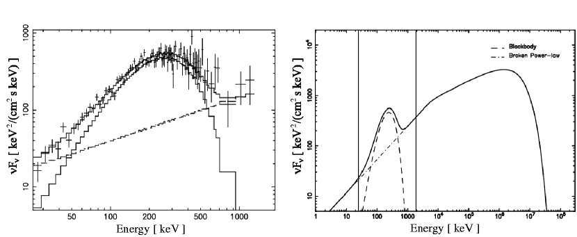
Figure 1: Time-resolved $\nu F_{\nu}$ spectra of GRB911016 assumed to have a strong high-energy component in the GeV-domain. See also figure 6. Left panel: XSPEC Hybrid model fit in BATSE energy band: 0.704 - 1.280 s. Right panel: SBM hybrid model simulation of the same burst extrapolated in the GLAST energy band: 1.0 - 1.1 s. The solid line describes the hybrid model, the dashed line the blackbody component and the dot-dashed line the broken power-law. The two vertical lines in the plot describe the energy range covered by BATSE.

In our simulations for GLAST we extended the energy range into the GLAST domain, and therefore used an extended time-dependent hybrid model that included a blackbody function that evolves over time and a broken power-law – instead of a single power-law component – with a high-energy cut-off. The blackbody component that evolves over time is described by:

$$N_{bb}(E,t)\,=\,A(t)_{bb}\,\frac{E^{2}\mathrm{d}E}{e^{E/kT(t)}-1}$$ (3)

We motivated the broken power-law based on the following two facts: a) OTS radiation may according to theory show a break in the energy domain covered by GLAST and b) power-law index values in the BATSE data from the hybrid model fits can be interpreted as being distributed around two values as shown in Battelino (2006).

Table 1: Power-law photon indices extracted with BATSE and used as input to SBM

GRB911016		GRB941026		GRB960530
Time range [s]	Index	Time range [s]	Index	Time range [s]	Index
0.000 - 3.520	$1.30\pm 0.05$	0.030 - 6.272	$1.57\pm 0.09$	0.029 - 18.624	$1.42\pm 0.07$
3.520 - 7.105	$1.69\pm 0.08$	6.272 - 14.784	$2.12\pm 0.04$	-	-

These two power law index values may be given a physical interpretation: the higher value ($\sim 2.1$) stems from a shock-accelerated distribution of electrons and the lower value ($\sim 1.5$) from the cooling electrons originating from the same distribution. The broken power-law component is described by:

$$N(E,t)_{bpo}\,=\,\begin{cases}A(t)_{bpo}\,(\frac{E}{1\,keV})^{p_{1}},\qquad\qquad\qquad\qquad\,\,\,\,E\,<\,E_{b}(t)\\ A(t)_{bpo}\,(\frac{E_{b}(t)}{1\,keV})^{p_{2}-p_{1}}\,(\frac{E}{1\,keV})^{-p_{2}},\qquad\quad E\,\geq\,E_{b}(t)\\ \end{cases}$$ (4)

A high-energy cut-off was assumed due to the competition between the acceleration of the electrons and the radiative cooling that leads to a maximal energy that the electrons can be accelerated to. The values chosen for the simulations were based on results by de Jager et al. (1996). Their studies show that the spectrum of the Crab nebula has a high-energy cut-off $e$-folding energy of $\sim$30 MeV, as predicted by their model. This is a robust value given by the model and independent of the magnetic field strength, $B$. We assumed, in our hybrid model implementation, that similar physical conditions exist at the GRB radiation site. Since the spectra from the prompt emission is boosted with a Lorentz-factor $\Gamma\sim 100$, we selected $e$-folding values of 5.0 GeV for GRB911016 and 3.0 GeV for GRB941026 and GRB960530. These values fall within the GLAST energy range and the extended hybrid model is therefore in the simulations described by:

$$N(E,t)\,=\,\begin{cases}N_{bb}(E,t)\,+\,N_{bpo}(E,t),\qquad\qquad\qquad\,\,\,\,E\,<\,E_{c}\\ N_{bb}(E,t)\,+\,N_{bpo}(E,t)\,e^{(E_{c}-E)/E_{e}},\qquad\,\,\,E\,\geq\,E_{c}\\ \end{cases}$$ (5)

where $E_{c}$ is the energy from where the high-energy cutoff starts and $E_{e}$ the $e$-folding energy. Extra-galactic background light (EBL) is expected to contribute to a high-energy cut-off for GRBs, but we did not consider this $\gamma\gamma$ absorption process in our simulations. This absorption process may however be important in spectra from GRBs at large cosmical distances.

2.2 Modeling the temporal evolution

Kocevski et al. (2003) show that the FRED light-curves associated with the temporal evolution of the flux of single pulse bursts may be described by:

$$F(t)\,=\,F_{m}\bigg{(}\,\frac{t}{t_{m}}\,\bigg{)}^{r}\,\bigg{[}\frac{d}{d+r}\,+\,\frac{r}{d+r}\,\bigg{(}\frac{t}{t_{m}}\bigg{)}^{r+1}\bigg{]}^{-(r+d)/(r+1)}$$ (6)

where $F_{m}$ is maximum flux, $t_{m}$ the time at maximum flux, $r$ the dimensionless power-law index describing the rise phase and $d$ the corresponding index for the decay phase. The power-law describing the rise phase is in equation (6) proportional to $t^{r}$ while the decay phase is described by:

$$F(t)\,=\,F_{0}\,\big{[}1+\frac{t}{T(d-1)}\big{]}^{-d}$$ (7)

as suggested by Ryde and Svensson (2000, 2002) for single pulse bursts. $F_{0}$ is here the flux at the start of the decay phase and $T$ a normalization parameter. By utilizing the Levenberg-Marquardt algorithm we extracted the $r$ and $d$ parameters using equation (6) for the BATSE flux of each model component (blackbody and single power-law) over the energy range 20 keV-1 MeV for the three bursts.

Table 2: Temperature parameters used as input to SBM

		GRB911016	GRB941026	GRB960530
$kT_{n}$	[keV]	67.23	67.6	37.38
$t_{n}$	[s]	0.992	0.960	2.392
$t_{0}$	[s]	$1.24\pm 0.06$	$2.1\pm 0.2$	$3.0\pm 0.3$
a		$-0.04\pm 0.03$	$0.0$	$-0.22\pm 0.05$
b		$-0.48\pm 0.02$	$-0.35\pm 0.02$	$-0.65\pm 0.04$
$\delta$		$0.08$	$0.2\pm 0.1$	0.02

Ryde shows in Ryde (2004) that $kT$ in equation (3) is a function of time that often follows a smoothly broken power-law with an initial power-law index $a$ and a later index $b$:

$$kT(t)\,=\,kT_{n}\,\bigg{(}\frac{t}{t_{n}}\bigg{)}^{\phi}\,\bigg{(}\frac{\cosh[\log(t/t_{0})/\delta]}{\cosh[\log(t_{n}/t_{0})/\delta]}\bigg{)}^{\xi\delta\ln 10}$$ (8)

where $t_{0}$ is the time of the break, $\delta$ is the width of the transition, $\xi\,=\,(b-a)/2$, and $\phi\,=\,(b+a)/2$. Equation (8) was used to extract the temporal parameters associated with the blackbody component in the hybrid model. The results from the fitting procedure, also here using a Levenberg-Marquardt method, are presented in table 2.

The power-law indices, for all three bursts, exhibited some form of temporal evolution, but it was – due to the large variance for each individual data point – hard to determine whether the index was smoothly changing over time or in discrete steps. One interpretation of the varying power-law index is that the break in synchrotron radiation spectrum – that stem from a shock-accelerated electron distribution (higher energy power-law index) and from cooling electrons (lower energy power-law index) – moves or jumps across the BATSE energy window as the burst progresses. For GRB911016 and GRB941026 we simulated the temporal evolution of the power-law break with the following equation:

$$E_{n}(t)\,=\,(\,E_{n,0}\,-\,E_{n,\infty}\,)\,e^{-t/t_{n}}\,+\,E_{n,\infty}$$ (9)

where $E_{n,0}$ is the initial energy at time $t=0$, $E_{n,\infty}$ the asymptotic final energy when $t$ tends to infinity and $t_{n}$ the rate scaling factor. This equation is neither empirically nor analytically deduced, and is only motivated by it being a candidate for describing the observed evolution. The power-law component in GRB960530 could be well fitted with a constant value and we did therefore not implement any temporal evolution of its power-law break. We implemented, however, for this simulation of GRB960530 a fixed break at 6.0 MeV, with a high-energy power-law index of 2.1, as shown in figure 2.

3 Simulating the thermal GRBs

A generic C++ framework, Simple Burst Modeler (SBM), was developed in order to simulate the spectral evolution of the bursts covering the GLAST energy range. SBM produces histogram files, one for each detector-type on-board GLAST, that describe the amount of photons produced by the simulated burst binned in energy and time. The right panel in figure 1 show the time-resolved spectrum of the simulated GRB911016 while figure 2 shows burst data simulated for GRB960530.

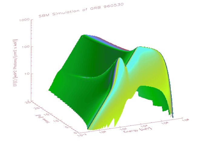
Figure 2: Evolution of the $\nu F_{\nu}$ spectrum over time in the keV-GeV range for a simulated GRB. The simulation is based on sub-MeV data collected by BATSE onboard CGRO for GRB960530. The blackbody peak can be seen around 100 keV, the power-law break around 10 MeV and the high-energy cutoff in the GeV domain.

The histogram file produced for the LAT instrument is then fed into gtobssim, the LAT fast observation simulator, and the NaI and BGO histogram files into GBM Tools, the GBM simulator. A modified version of gtobssim was used so that generic histogram files of the type produced by SBM could be read in and used in the simulations. When running gtobssim we used the LAT instrument response file produced for Data Challenge 2 (DC2) in our simulations. GBM Tools was also modified with the added capabilities to output the detector energy grids into files required by SBM and to read in the histogram files produced by SBM.

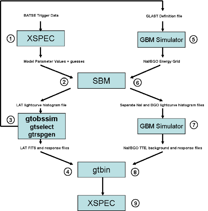
Figure 3: Combined SBM and GLAST simulation procedure. Note that gtobssim has to be executed before the GBM Simulator since the definition file required by the GBM simulation package is created by the GLAST ScienceTools in connection to the LAT simulation run.

Figure 3 summarizes the steps that were performed for each simulated burst. These seemingly awkward steps were needed since gtobssim produces a definition file used as input to GBM tools and GBM tools create energy grid files required by SBM.

1. XSPEC was first used to analyze the BATSE data in order to extract the necessary parameters used as input to SBM.

2. SBM was executed to produce a LAT histogram file.

3. gtobssim used the LAT histogram as input to produce the LAT FITS and response files, as well as the burst definition file. gtobssim also needs a response function and a template that describes the position of the burst relative to the GLAST spacecraft. During our simulations the response function for DC2 was used. We also utilized the same template in all simulations hence positioning all three bursts at $\theta=62.9^{\circ}$ and $\phi=95.3^{\circ}$, where $\theta$ and $\phi$ represents the inclination angle to the normal of the LAT detector and azimuthal angle around the LAT normal respectively. gtselect was used to select the events of interest and gtrspgen to produce the response files readable by XSPEC.

4. gtbin was executed in order to create the FITS files in the PHA format readable by XSPEC. At this point all LAT data was produced.

5. The GBM Simulator was now executed with the GLAST definition file as input, at this time only producing NaI and BGO energy grid files.

6. SBM was executed again to produce histogram files that was used as input to the GBM simulator. The same parameter data was used as previously for the LAT run, but this time with the additional BGO and NaI energy grid files as input.

7. The GBM Simulator was fed with the SBM histogram files producing Time-Triggered Event (TTE) files as well as background and response files.

8. gtbin was now utilized again but this time on the files produced by the GBM simulator converting them to the PHA format readable by XSPEC.

9. The produced LAT data and GBM data were now jointly analyzed with XSPEC.

4 Results

XSPEC was utilized on the data produced by gtobssim and GBM tools by imposing the extended hybrid model, as described by equation (5), on the time-integrated spectra from two NaI detectors, one BGO detector and the LAT instrument. Both $\chi^{2}$ and C statistic, a modified version of Cash statistic (see Cash, 1979; Arnaud and Dorman, 2003), was used in our analysis to estimate parameters that covered the first five seconds from trigger, while only $\chi^{2}$ statistic was used for the model test. C statistic give better results than $\chi^{2}$ at count rates below 10 counts per bin, but can not, as opposed to $\chi^{2}$ tests, be used to get a ”goodness-of-fit”. It is therefore primarily used for estimation of parameter values. C statistic also assumes that the error on the counts is pure Poissonian, and should hence be the preferred statistic when estimating parameter values based on data with low photon counts. At higher count rates, both $\chi^{2}$ and C statistic are expected to give the same parameter estimates, assuming we are dealing with Gaussian distributions. The $\chi^{2}$ model analysis was performed on both ungrouped and grouped data. In the latter case, the data was grouped into bins with at least 10 photons per bin for all detectors. Some of the results, from our analysis using $\chi^{2}$ and C statistic, are presented in table 3.

Table 3: Parameter values from hybrid model fit on simulated GLAST data

Burst	Statistic	Blackbody	Powerlaw	Powerlaw	Model Statistics
		Temp [keV]	Index 1	Index 2	$\nu$	$\chi^{2}_{\nu}$	$P$
GRB911016	$\chi^{2}_{u}$	$53.3\pm 1.1$	$1.30\pm 0.04$	$1.71\pm 0.03$	336	0.90	0.92
	$\chi^{2}_{g}$	$53.8\pm 1.1$	$1.25\pm 0.04$	$1.76\pm 0.03$	206	0.98	0.55
	C	$53.9\pm 1.1$	$1.26\pm 0.04$	$1.74\pm 0.03$	-	-	-
GRB941026	$\chi^{2}_{u}$	$59.2\pm 1.3$	1.6 (frozen)	2.1 (frozen)	339	0.82	0.99
	$\chi^{2}_{g}$	$61.5\pm 1.3$	$1.71\pm 0.03$	$2.9\pm 0.8$	228	0.82	0.98
	C	$61.0\pm 1.3$	$1.69\pm 0.02$	$2.4\pm 0.2$	-	-	-
GRB960530	$\chi^{2}_{u}$	$41.8\pm 0.8$	$1.48\pm 0.02$	$2.4\pm 0.2$	336	0.91	0.87
	$\chi^{2}_{u}$	$41.8\pm 0.8$	$1.42$ (frozen)	2.1 (frozen)	339	0.96	0.70
	$\chi^{2}_{g}$	$41.7\pm 0.9$	$1.44\pm 0.02$	$2.3\pm 0.1$	208	1.03	0.36
	C	$41.5\pm 0.9$	$1.42\pm 0.01$	$2.2\pm 0.1$	-	-	-

Figures 4 and 5 show a simulated photon spectrum, based on BATSE data for GRB911016, together with the fit of the extended hybrid model. The left panel in figure 6 shows the $\nu F_{\nu}$ spectrum for the same burst. The resulting fit parameters were, for each simulated burst, compared with the SBM input parameters. The simulated GRB911016 output parameters was consistent with the SBM input parameter values. Table 3 presents some of the parameter values and also the reduced $\chi^{2}$- ($\nu$ represents the degrees of freedom) and $P$-values from the hybrid model fits. All the fits showed reduced $\chi^{2}$ values around 1.0 and with high $P$-values, close to 1.0, for the ungrouped data. The high $P$-values indicate that the errors for the ungrouped data points, used in our XSPEC fits, are over-estimated. Grouping the data into at least 10 photons per bin, decreased the $P$-values and also gave $\chi^{2}$-statistic parameter estimates closer to the values found when using C-statistic. The right panel in figure 6 shows the $\chi^{2}$ confidence regions (with $1\sigma$, $2\sigma$ and $3\sigma$ levels) for the power-law photon-index versus the blackbody temperature $kT$. It shows a consistency between the BATSE data and the simulated GLAST data for the modeled temperature. The temperature was also consistent with the input data for the other two bursts, but the mean value for the photon indices became slightly softer in the GLAST data fits. This is probably due to the evolution of the blackbody temperature and, in the case of GRB941026, the evolution of the break-energy of the power-law. Freezing the indices to the expected values, when analyzing the ungrouped data, we still received good statistics $\chi^{2}\lesssim 1.0$, and consistency with the input parameters. This can be seen for GRB960530 in table 3. It was however not possible to determine the confidence levels for the high-energy cut-off parameters in the fit – neither with binned $\chi^{2}$ nor C statistic – due to the low photon count at the higher energies.

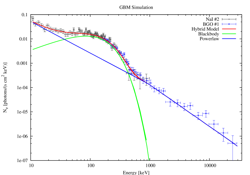
Figure 4: Unfolded photon-spectrum from one NaI and one BGO detector of the GBM instrument covering the first five seconds of the simulated burst. The fitted two components of the hybrid model are also shown in this figure. The fit was performed on ungrouped data using $\chi^{2}$ statistic. The simulation was based on BATSE data for GRB911016. Note that the data points have been grouped in the plot.

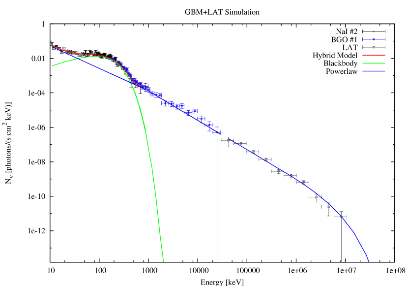
Figure 5: The same simulated burst as in figure 4, including LAT data. The fit was performed on ungrouped data using $\chi^{2}$ statistic. Note that the data points has been grouped in the plot.

Figure 6: Burst data was simulated with SBM using parameters extracted from BATSE data for GRB911016. The SBM generated data was then used in the GBM and LAT observation simulations. Left panel: $\nu F_{\nu}$ plot resulting from a fit of hybrid model from two NaI, one BGO detector and the LAT detector. This time-bin includes data from the first five seconds from the trigger. The fit was performed on ungrouped data using $\chi^{2}$ statistic. Note that the data points has been grouped in the plot after the fit. See also figure 1. Right panel: $\chi^{2}$ confidence regions for hybrid model fits with $1\sigma$, $2\sigma$ and $3\sigma$ levels. Photon index versus blackbody temperature for GRB911016 observed by BATSE (covering 0.029 - 4.864 s) have dotted contours and upper cross covering. The corresponding confidence regions for the simulated data for GLAST (covering 0.0 - 5.0 s) has solid contours and the lower cross. All parameters in the extended hybrid model were frozen except for the blackbody temperature ($kT$) and power-law photon index when the XSPEC steppar procedure was used. The parameter estimation was performed on ungrouped data.

5 Discussion

The hybrid model, that may be interpreted as a combination of photospheric and optically-thin synchrotron radiation, fits the spectra of single-pulsed GRBs well (see Ryde, 2005; Battelino, 2006). The problem with the synchrotron ”line of death” ($\alpha\,>\,-$2/3) is avoided with this model, since the Rayleigh-Jeans portion of the blackbody component explains the hard spectral slopes seen in many BATSE bursts. We presented here simulations of thermal bursts with a large super-MeV emission in the GLAST energy range using gtobssim and GBM tools. The simulations were followed by XSPEC analysis of the first five seconds of the resulting data for each burst, grouped to at least 10 photons per bin. This analysis showed that an applied thermal model, consisting of a blackbody function and a broken power-law with a high-energy cutoff, gave the desired ”goodness-of-fit” represented by the $P$-value close to 0.5 for all bursts. Parameter estimates of the power-law indices generally gave softer values than used for the simulation, but this can be explained by the temporal evolution of the blackbody peak and power-law break over the five seconds that were integrated into one spectrum. The simulations of GLAST data for thermal bursts hence show that a photospheric component should be clearly detected by the GLAST instruments, if it dominates in the energy window of the GBM instrument and is super-positioned over an optically-thin synchrotron ”background” spectrum extending from the lowest GBM energies into the LAT domain. The evolution of the Planck function will be possible to determine using events collected by the two detector types, NaI (8 keV - 1 MeV) and BGO (150 keV - 30 MeV), that constitute the GBM instrument. The non-thermal component will be detectable by both GBM and LAT.

From the simulated GLAST data of the three single-pulse bursts it was not possible to determine the 1$\sigma$ confidence region for the high-energy cut-off parameters due to the low photon count, not even when using C statistic. We therefore expect that the cut-off and $e$-folding energy for some bursts may be hard to determine, especially for time-resolved spectra, due to the low photon count, if the LAT instrument response function is similar to the one used for Data Challenge 2 (DC2), even if the cut-off lies within the LAT domain. Possibly better results could be reached using the raw event data or using a response function with more lean cuts than the ones used in DC2 for time-integrated spectra.

References

- Band et al. (1993) D. Band, et al., ApJ 413, 281–292 (1993).
- Crider et al. (1997) A. Crider, E. P. Liang, I. A. Smith, R. D. Preece, M. S. Briggs, G. N. Pendleton, W. S. Paciesas, D. L. Band, and J. L. Matteson, ApJ 479, L39+ (1997).
- Preece et al. (1998) R. D. Preece, et al., ApJ 506, L23–L26 (1998).
- Lloyd and Petrosian (2000) N. M. Lloyd, and V. Petrosian, ApJ 543, 722–732 (2000), astro-ph/0007061.
- Panaitescu and Mészáros (2000) A. Panaitescu, and P. Mészáros, ApJ 544, L17–L21 (2000), astro-ph/0009309.
- Medvedev (2000) M. V. Medvedev, ApJ 540, 704–714 (2000), astro-ph/0001314.
- Baring and Braby (2004) M. G. Baring, and M. L. Braby, ApJ 613, 460–476 (2004), astro-ph/0406025.
- Mészáros and Rees (2000) P. Mészáros, and M. J. Rees, ApJ 530, 292–298 (2000), astro-ph/9908126.
- Mészáros et al. (2002) P. Mészáros, E. Ramirez-Ruiz, M. J. Rees, and B. Zhang, ApJ 578, 812–817 (2002), astro-ph/0205144.
- Daigne and Mochkovitch (2002) F. Daigne, and R. Mochkovitch, MNRAS 336, 1271–1280 (2002), astro-ph/0207456.
- Drenkhahn and Spruit (2002) G. Drenkhahn, and H. C. Spruit, A&A 391, 1141–1153 (2002), astro-ph/0202387.
- Ryde (2004) F. Ryde, ApJ 614, 827–846 (2004).
- Ryde (2005) F. Ryde, ApJ 625, L95–L98 (2005), astro-ph/0504450.
- Rees and Mészáros (2005) M. J. Rees, and P. Mészáros, ApJ 628, 847–852 (2005), astro-ph/0412702.
- Ryde et al. (2006) F. Ryde, C.-I. Björnsson, Y. Kaneko, P. Mészáros, R. Preece, and M. Battelino, ApJ 652, 1400–1415 (2006), astro-ph/0608363.
- Ghirlanda et al. (2003) G. Ghirlanda, A. Celotti, and G. Ghisellini, A&A 406, 879–892 (2003).
- Arnaud and Dorman (2003) K. Arnaud, and B. Dorman, Xspec, an X-Ray Spectral Fitting Package, User’s Guide for version 11.3.x, NASA, 2003.
- González et al. (2003) M. M. González, B. L. Dingus, Y. Kaneko, R. D. Preece, C. D. Dermer, and M. S. Briggs, Nature 424, 749–751 (2003).
- Battelino (2006) M. Battelino, Simulation of the keV-GeV emission from gamma-ray bursts using a thermal emission model and its detectability by GLAST (2006), Master Thesis, Department of Astronomy, Stockholm University.
- de Jager et al. (1996) O. C. de Jager, A. K. Harding, P. F. Michelson, H. I. Nel, P. L. Nolan, P. Sreekumar, and D. J. Thompson, ApJ 457, 253–+ (1996).
- Kocevski et al. (2003) D. Kocevski, F. Ryde, and E. Liang, ApJ 596, 389–400 (2003).
- Ryde and Svensson (2000) F. Ryde, and R. Svensson, ApJ 529, L13–L16 (2000).
- Ryde and Svensson (2002) F. Ryde, and R. Svensson, ApJ 566, 210–228 (2002).
- Cash (1979) W. Cash, ApJ 228, 939–947 (1979).