Supersymmetric methods in the traveling variable: inside neurons and at the brain scale

Abstract

We apply the mathematical technique of factorization of differential operators to two different problems. First we review our results related to the supersymmetry of the Montroll kinks moving onto the microtubule walls as well as mentioning the sine-Gordon model for the microtubule nonlinear excitations. Second, we find analytic expressions for a class of one-parameter solutions of a sort of diffusion equation of Bessel type that is obtained by supersymmetry from the homogeneous form of a simple damped wave equations derived in the works of P.A. Robinson and collaborators for the corticothalamic system. We also present a possible interpretation of the diffusion equation in the brain context.

1 Nonlinear biological excitations

The possibility of soliton excitations in biological structures has been first pointed out by Englander et al [1] in 1980 who speculated that the so-called ‘open states’ units made of approximately ten adjacent open pairs in long polynucleotide double helices could be thermally induced solitons of the double helix due to a coherence of the twist deformation energy. Since then a substantial amount of literature has been accumulating on the biological significance of DNA nonlinear excitations (for a recent paper, see [2]). On the other hand, the idea of nonlinear excitations has emerged in 1993 in the context of the microtubules (MTs) [3], the dimeric tubular polymers that contribute the main part of the eukaryotic cytoskeleton. In the case of neurons, MTs are critical for the growth and maintenance of axons. It is known that axonal MTs are spatially organized but are not under the influence of a MT-organizing center as in other cells. We also remind that in 1995 Das and Schwarz have used a two-dimensional smectic liquid crystal model to show the possibility of electrical solitary wave propagation in cell membranes [4]. Nevertheless, there is no clear experimental evidence at the moment of any of these biological solitons and kinks.

2 Supersymmetric MT Kinks

Based on well-established results of Collins, Blumen, Currie and Ross [5] regarding the dynamics of domain walls in ferrodistortive materials, Tuszyński and collaborators [3, 6] considered MTs to be ferrodistortive and studied kinks of the Montroll type [7] as excitations responsible for the energy transfer within this highly interesting biological context.

The Euler-Lagrange dimensionless equation of motion of ferrodistortive domain walls as derived in [5] from a Ginzburg-Landau free energy with driven field and dissipation included is of the travelling reaction-diffusion type

$$\psi^{{}^{\prime\prime}}+\rho\psi^{{}^{\prime}}-\psi^{3}+\psi+\sigma=0~{},$$ (1)

where the primes are derivatives with respect to a travelling coordinate $\xi=x-vt$, $\rho$ is a friction coefficient and $\sigma$ is related to the driven field [5].

There may be ferrodistortive domain walls that can be identified with the Montroll kink solution of Eq. (1)

$$M(\xi)=\alpha_{1}+\frac{\sqrt{2}\beta}{1+\exp(\beta\xi)}~{},$$ (2)

where $\beta=(\alpha_{2}-\alpha_{1})/\sqrt{2}$ and the parameters $\alpha_{1}$ and $\alpha_{2}$ are two nonequal solutions of the cubic equation

$$(\psi-\alpha_{1})(\psi-\alpha_{2})(\psi-\alpha_{3})=\psi^{3}-\psi-\sigma~{}.$$ (3)

Rosu has noted that Montroll’s kink can be written as a typical $\tanh$ kink [8]

$$M(\xi)=\gamma-\tanh\left(\frac{\beta\xi}{2}\right)~{},$$ (4)

where $\gamma\equiv\alpha_{1}+\alpha_{2}=1+\frac{\alpha_{1}\sqrt{2}}{\beta}$. The latter relationship allows one to use a simple construction method of exactly soluble double-well potentials in the Schrödinger equation proposed by Caticha [9]. The scheme is a non-standard application of Witten’s supersymmetric quantum mechanics [10] having as the essential assumption the idea of considering the $M$ kink as the switching function between the two lowest eigenstates of the Schrödinger equation with a double-well potential. Thus

$$\phi_{1}=M\phi_{0}~{},$$ (5)

where $\phi_{0,1}$ are solutions of $\phi^{{}^{\prime\prime}}_{0,1}+[\epsilon_{0,1}-u(\xi)]\phi_{0,1}(\xi)=0$, and $u(\xi)$ is the double-well potential to be found.

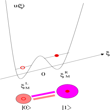
Figure 1: Single electron within the traveling double-well potential $u(\xi)$ as a qubit. The electron can switch from one wall to another by tunneling and the relation between the wavefunctions in the two wells is given by Eq. (5).

Substituting Eq. (5) into the Schrödinger equation for the subscript 1 and substracting the same equation multiplied by the switching function for the subscript 0, one obtains

$$\phi^{{}^{\prime}}_{0}+R_{M}\phi_{0}=0~{},$$ (6)

where $R_{M}$ is given by

$$R_{M}=\frac{M^{{}^{\prime\prime}}+\epsilon M}{2M^{{}^{\prime}}}~{},$$ (7)

and $\epsilon=\epsilon_{1}-\epsilon_{0}$ is the lowest energy splitting in the double-well Schrödinger equation. In addition, notice that Eq. (6) is the basic equation introducing the superpotential $R$ in Witten’s supersymmetric quantum mechanics, i.e., the Riccati solution. For Montroll’s kink the corresponding Riccati solution reads

$$R_{M}(\xi)=-\frac{\beta}{2}{\rm tanh}\left(\frac{\beta}{2}\xi\right)+\frac{\epsilon}{2\beta}\Bigg{[}\sinh(\beta\xi)+2\gamma\cosh^{2}\left(\frac{\beta}{2}\xi\right)\Bigg{]}$$ (8)

and the ground-state Schrödinger function is found by means of Eq. (6)

$$\phi_{0,M}(\xi) = \phi_{0}(0)\cosh\left(\frac{\beta}{2}\xi\right)\exp\left(\frac{\epsilon}{2\beta^{2}}\right)\exp\left(-\frac{\epsilon}{2\beta^{2}}\Big{[}\cosh(\beta\right.\xi)$$ (9)

$$\left.-\gamma\beta\xi-\gamma\sinh(\beta\xi)\Big{]}\right)~{},$$

while $\phi_{1}$ is obtained by switching the ground-state wave function by means of $M$. This ground-state wave function is of supersymmetric type

$$\phi_{0,M}(\xi)=\phi_{0,M}(0)\exp\Bigg{[}-\int_{0}^{\xi}R_{M}(y)dy\Bigg{]}~{},$$ (10)

where $\phi_{0,M}(0)$ is a normalization constant.

The Montroll double well potential is determined up to the additive constant $\epsilon_{0}$ by the ‘bosonic’ Riccati equation

$$u_{M}(\xi) = R_{M}^{2}-R_{M}^{{}^{\prime}}+\epsilon_{0}=\frac{\beta^{2}}{4}+\frac{(\gamma^{2}-1)\epsilon^{2}}{4\beta^{2}}+\frac{\epsilon}{2}+\epsilon_{0}$$ (11)

$$+\frac{\epsilon}{8\beta^{2}}\Big{[}\left(4\gamma^{2}\epsilon+2(\gamma^{2}+1)\epsilon{\rm cosh}(\beta\xi)-8\beta^{2}\right){\rm cosh}(\beta\xi)$$

$$-4\gamma\left(\epsilon+\epsilon{\rm cosh}(\beta\xi)-2\beta^{2}\right){\rm sinh}(\beta\xi)\Big{]}.$$

If, as suggested by Caticha, one chooses the ground state energy to be

$$\epsilon_{0}=-\frac{\beta^{2}}{4}-\frac{\epsilon}{2}+\frac{\epsilon^{2}}{4\beta^{2}}\left(1-\gamma^{2}\right)~{},$$ (12)

then $u_{M}(\xi)$ turns into a travelling, asymmetric Morse double-well potential of depths depending on the Montroll parameters $\beta$ and $\gamma$ and the splitting $\epsilon$

$$U_{0,m}^{L,R}=\beta^{2}\Bigg{[}1\pm\frac{2\epsilon\gamma}{(2\beta)^{2}}\Bigg{]}~{},$$ (13)

where the subscript $m$ stands for Morse and the superscripts $L$ and $R$ for left and right well, respectively. The difference in depth, the bias, is $\Delta_{m}\equiv U_{0}^{L}-U_{0}^{R}=2\epsilon\gamma$, while the location of the potential minima on the traveling axis is at

$$\xi_{m}^{L,R}=\mp\frac{1}{\beta}\ln\Bigg{[}\frac{(2\beta)^{2}\pm 2\epsilon\gamma}{\epsilon(\gamma\mp 1)}\Bigg{]}~{},$$ (14)

that shows that $\gamma\neq\pm 1$.

An extension of the previous results is possible if one notices that $R_{M}$ in Eq. (8) is only the particular solution of Eq. (11). The general solution is a one-parameter function of the form

$$R_{M}(\xi;\lambda)=R_{M}(\xi)+\frac{d}{d\xi}\Big{[}\ln(I_{M}(\xi)+\lambda)\Big{]}$$ (15)

and the corresponding one-parameter Montroll potential is given by

$$u_{M}(\xi;\lambda)=u_{M}(\xi)-2\frac{d^{2}}{d\xi^{2}}\Big{[}\ln(I_{M}(\xi)+\lambda)\Big{]}~{}.$$ (16)

In these formulas, $I_{M}(\xi)=\int^{\xi}\phi_{0,M}^{2}(\xi)d\xi$ and $\lambda$ is an integration constant that is used as a deforming parameter of the potential and is related to the irregular zero mode. The one-parameter Darboux-deformed ground state wave function can be shown to be

$$\phi_{0,M}(\xi;\lambda)=\sqrt{\lambda(\lambda+1)}\frac{\phi_{0,M}}{I_{M}(\xi)+\lambda}~{},$$ (17)

where $\sqrt{\lambda(\lambda+1)}$ is the normalization factor implying that $\lambda\notin[0,-1]$. Moreover, the one-parameter potentials and wave functions display singularities at $\lambda_{s}=-I_{M}(\xi_{s})$. For large values of $\pm\lambda$ the singularity moves towards $\mp\infty$ and the potential and ground state wave function recover the shapes of the non-parametric potential and wave function. The one-parameter Morse case corresponds formally to the change of subscript $M\rightarrow m$ in Eqs. (15) and (16). For the single well Morse potential the one-parameter procedure has been studied by Filho [12] and Bentaiba et al [13].

The one-parameter extension leads to singularities in the double-well potential and the corresponding wave functions. If the parameter $\lambda$ is positive the singularity is to be found on the negative $\xi$ axis, while for negative $\lambda$ it is on the positive side. Potentials and wave functions with singularities are not so strange as it seems [14] and could be quite relevant even in nanotechnology where quantum singular interactions of the contact type are appropriate for describing nanoscale quantum devices. We interpret the singularity as representing the effect of an impurity moving along the MT in one direction or the other depending on the sign of the parameter $\lambda$. The impurity may represent a protein attached to the MT or a structural discontinuity in the arrangement of the tubulin molecules. This interpretation of impurities has been given by Trpišová and Tuszyński in non-supersymmetric models of nonlinear MT excitations [15].

3 The sine-Gordon MT solitons

Almost simultaneously with Sataric, Tuszynski and Zakula, there was another group, Chou, Zhang and Maggiora [16], who published a paper on the possibility of kinklike excitations of sine-Gordon type in MTs but in a biological journal. Even more, they assumed that the kink is excited by the energy released in the hydrolysis of GTP $\rightarrow$ GDP in microtubular solutions. As the kink moves forward, the individual tubulin molecules involved in the kink undergo motion that can be likened to the dislocation of atoms within the crystal lattice.

They performed an energy estimation showing that a kink in the system possesses about 0.36 - 0.44 eV, which is quite close to the 0.49 eV of energy released from the hydrolysis of GTP.

Moreover, they assumed that the interaction energy $U(r)$ between two neighboring tubulin molecules along a protofilament is harmonic:

$$U(r)\approx\frac{1}{2}k(r-a_{0})^{2}~{},$$ (18)

where $k=\frac{d^{2}U(a_{0})}{dr^{2}}$ and $r=x_{i}-x_{i-1}$. In addition to this kind of nearest neighbor interaction, a tubulin molecule is also subjected to interactions with the remaining tubulin molecules of the MT, i.e., those in the same protofilament but not nearest neighbor to it.

Chou et al cite pages 425-427 in the book of R.K. Dodd et al (Solitons and Nonlinear Wave Equations, Academic Press 1982) for the claiming that this interaction for the $i$th tubulin molecule of a protofilament can be approximated by the following periodic effective potential

$$U_{i}=U_{0}\left(1-\cos\frac{2\pi\xi_{i}}{a_{0}}\right)~{},$$ (19)

where $U_{0}$ is the half-height of the potential energy barrier and $\xi_{i}$ is the displacement of the $i$th tubulin molecule from the equilibrium position within a particular protofilament.

Introducing the new variable $\phi_{i}=\frac{2\pi}{a_{0}}\xi_{i}$ the following sine-Gordon equation is obtained

$$m\frac{\partial^{2}\phi}{\partial t^{2}}=ka_{0}^{2}\frac{\partial^{2}\phi}{\partial x^{2}}-\left(\frac{2\pi}{a_{0}}\right)^{2}U_{0}\sin\phi~{}$$ (20)

that can be reduced to the standard form of the sine-Gordon equation

$$\frac{\partial^{2}\phi}{\partial x^{2}}-\frac{1}{c^{2}}\frac{\partial^{2}\phi}{\partial t^{2}}=\frac{1}{l^{2}}\sin\phi$$ (21)

if one sets $c^{2}=\frac{ka_{0}^{2}}{m}$ and $l^{-2}=\frac{4\pi^{2}U_{0}}{ka_{0}^{4}}$. Now, it is well known that the sine-Gordon equation has the famous inverse tangent kink solution

$$\phi=\tan^{-1}\left(\exp[\pm\frac{\gamma}{l}(x-vt)]\right)~{},$$ (22)

where $\gamma=\frac{1}{\sqrt{1-\frac{v^{2}}{c^{2}}}}$ is an acoustic Lorentz factor and $w=\frac{\gamma}{l}$ is the kink width.

Most interestingly, the momentum of a tubulin dimer is strongly localized:

$$p=\frac{d(m\xi)}{dt}=\frac{ma_{0}}{\pi}\frac{\gamma v}{l}{\rm sech}\bigg{[}-\frac{\gamma}{l}(x-vt)\bigg{]}~{}.$$ (23)

This momentum function possesses a very high and narrow peak at the center of the kink width implying that the corresponding tubulin molecule will have maximum momentum when it is at the top of the periodic potential. According to Chou et al this remarkable feature occurs only in nonlinear wave mechanics.

Interestingly, for purposes of illustration, these authors have assumed the width of a kink $w\approx 3a_{0}$. Therefore, with the kink moving forward, the affected region always involves three tubulin molecules. For a general case, however, the width $w$ of a kink can be calculated from

$$w=\frac{a_{0}}{2\pi}\sqrt{\frac{ka_{0}^{2}}{U_{0}}}~{},$$ (24)

if the force constant $k$ between two neighboring tubulin molecules along a protofilament, the distance $a_{0}$ of their centers, and the energy barrier $2U_{0}$ of the periodic, effective potential are known. Then the number of tubulin molecules involved in a kink is given by

$$\frac{w}{a_{0}}=(2\pi)^{-1}\sqrt{ka_{0}^{2}/U_{0}}~{}.$$ (25)

It is further known that the tubulin molecules in a MT are held by noncovalent bonds, therefore the interaction among them might involve hydrogen bonds, van der Waals contact, salt bridges, and hydrophobic interactions.

It was found by Israelachvili and Pashley [17] that the hydrophobic force law over the distance range 0-10 nm at 21^oC is well described by

$$\frac{F_{H}}{R}=Ce^{-D/D_{0}}\,N/m~{},$$ (26)

where $D$ is the distance between tubulin molecules, $D_{0}$ is a decay length, and $R=\frac{R_{1}R_{2}}{R_{1}+R_{2}}$ is a harmonic mean radius for two hydrophobic solute molecules, all in nm. $R$ is 4 nm in the case of tubulin.

3.1 More on the hydrolysis and solitary waves in MTs

Inside the cell, the MTs exist in an unstable dynamic state characterized by a continuous addition and dissociation of the molecules of tubulin. The polypeptides $\alpha$ and $\beta$ tubulin each bind one molecule of guanine nucleotide with high affinity. The nucleotide binding site on $\alpha$ tubulin binds GTP nonexchangeably and is referred to as the N site. The binding site on $\beta$ tubulin exchanges rapidly with free nucleotide in the tubulin heterodimer and is referred to as the E site.

Thus, the addition of each tubulin is accompanied by the hydrolysis of GTP 5’ bound to the $\beta$ monomer. In this reaction an amount of energy of $6.25\times 10^{-21}$ J is freed that can travel along MTs as a kinklike solitary wave.

The exchangeable GTP hydrolyses very soon after the tubulin binds to the MT. At $pH=7$ this reaction takes place according to the formula:

$$GTP^{4-}+H_{2}O\rightarrow GDP^{3-}+HPO_{4}^{2-}+H^{+}+\Delta_{H}E~{}.$$ (27)

The last mathematical formulation of the manner in which the energy $\Delta_{H}E$ is turned into a kink excitation claims that the hydrolysis causes a dynamical transition in the structure of tubulin [18].

4 Quantum information in the MT walls

Biological information processing, storage, and transduction occurring by computer-like transfer and resonance among the dimer units of MTs have been first suggested by Hamerrof and Watt [19] and enjoys much speculative activity [20].

For the case of sine-Gordon solitons, the information transport has been investigated by Abdalla et al [21].

Recently Shi and collaborators [22] worked out a processing scheme of quantum information along the MT walls by using previous hints of Lloyd for two-level pseudospin systems [23]. The MT wall is treated as a chain of three types of two pseudospin-state dimers. A set of appropriate resonant frequencies has been given. They conclude that specific frequencies of laser pulse excitations can be applied in order to generate quantum information processing.

Lloyd’s scheme uses the driving of a quantum computer by means of a sequence of laser pulses. He assumes a 1-dimensional arrangement of atoms of two types (A and B) that could be each of them in one of two states and are affected only by nearest neighbors. Then, information processing could be performed by laser pulses of specific frequencies $\omega_{K_{\alpha,\beta}}$, that change the state of the atom of the K kind (A or B type) if in a pair of atoms AB, A is in $\alpha$ state and B is in state $\beta$.

5 Supersymmetry at the Brain Scale

Neuronal activity is the result of the propagation of impulses generated at the neuron cell body and transmitted along axons to other neurons. Recently, Robinson and collaborators [25] obtained simple damped wave equations for the axonal pulse fields propagating at speed $v_{a}$ between two populations, $a$ and $b$, of neurons in the thalamocortical region of the brain. The explicit form of their equation is

$$\hat{O}_{R}\phi_{a}(t)=S[V_{a}(t)]~{},$$ (28)

where

$$\hat{O}_{R}=\left(\frac{1}{\nu_{a}^{2}}\frac{d^{2}}{dt^{2}}+\frac{2}{\nu_{a}}\frac{d}{dt}+1-r_{a}^{2}\nabla^{2}\right)~{},$$ (29)

where $\nu_{a}=v_{a}/r_{a}$, $r_{a}$ is the mean range of axons $a$, and $V_{a}=\sum_{b}V_{ab}$ is a so-called cell body potential which results from the filtered dendritic tree inputs. Robinson has used the experimental parameters in this equation for the processing of the experimental data. In the following we concentrate on a particular mathematical aspect of this equation and refer the reader to the works of Robinson’s group for more details concerning this equation.

5.1 The homogeneous equation

We treat first the homogeneous case, i.e., $S=0$ and we discard the subindexes as being related to the phenomenology not to the mathematics. Let us employ the change of variable $z=ax+by-ct$ (see, e.g., [26]), which is a traveling coordinate in 2+1 dimensions. This is justified because it was noticed by Wilson and Cowan [24] that distinct anatomical regions of cerebral cortex and of thalamic nuclei are functionally two-dimensional although extending to three spatial coordinates is trivial. We have the following rescalings of functions: $\phi_{t}=-c\phi_{z}$, $\phi_{tt}=v^{2}\phi_{zz}$, $\phi_{xx}=a^{2}\phi_{zz}$, $\phi_{yy}=b^{2}\phi_{zz}$. Then, we get the ordinary differential equation corresponding to the damped wave equation in the following form

$$\hat{O}_{R,z}\phi\equiv\left(\frac{d^{2}}{dz^{2}}-2\mu\frac{d}{dz}+\mu^{2}\right)\phi=\alpha^{2}\phi~{},$$ (30)

where

$$\mu=\frac{\nu c}{c^{2}-\nu^{2}r^{2}(a^{2}+b^{2})}~{},\qquad\alpha^{2}=\frac{\nu^{4}r^{2}(a^{2}+b^{2})}{[c^{2}-\nu^{2}r^{2}(a^{2}+b^{2})]^{2}}~{}.$$ (31)

The simple damped oscillator equation (30) can be easily factorized

$$L_{\mu}^{2}\phi\equiv\left(\frac{d}{dz}-\mu\right)\left(\frac{d}{dz}-\mu\right)\phi=\alpha^{2}\phi~{}.$$ (32)

The case $c^{2}<\nu^{2}r^{2}(a^{2}+b^{2})$ implies $\mu<0$ and the general solution of (30) can be written

$$\phi(z)=e^{\mu z}(Ae^{\alpha z}+Be^{-\alpha z})~{}.$$ (33)

The opposite case $c^{2}>\nu^{2}r^{2}(a^{2}+b^{2})$ will lead to only a change of sign in front of $\mu$ in all formulas henceforth, whereas the case $c^{2}=\nu^{2}r^{2}(a^{2}+b^{2})$ will be considered as nonphysical. The non-uniqueness of the factorization of second-order differential operators has been exploited in a previous paper [27] on the example of the Newton classical damped oscillator, i.e.,

$$\hat{N}y\equiv\left(\frac{d^{2}}{dt^{2}}+2\beta\frac{d}{dt}+\omega_{0}^{2}\right)y=0~{},$$ (34)

which is similar to the equation (30), unless the coefficient $2\beta$ is the friction constant per unit mass, $\omega_{0}$ is the natural frequency of the oscillator, and the independent variable is just time not the traveling variable. Proceeding along the lines of [27], one can search for the most general isospectral factorization

$$(D_{z}+f(z))(D_{z}+g(z))\phi=\alpha^{2}\phi~{}.$$ (35)

After simple algebraic manipulations one finds the conditions $f+g=-2\mu$ and $dg/dz+fg=\mu^{2}$ having as general solution $f_{\lambda}=\frac{\lambda}{\lambda z+1}-\mu$, whereas $f_{0}=-\mu$ is only a particular solution. Using the general solution $f_{\lambda}$ we get

$$\hat{A}_{+\lambda}\hat{A}_{-\lambda}\phi\equiv\left(D_{z}+\frac{\lambda}{\lambda z+1}-\mu\right)\left(D_{z}-\frac{\lambda}{\lambda z+1}-\mu\right)\phi=\alpha^{2}\phi~{}.$$ (36)

This equation does not provide anything new since it is just equation (31). However, a different operator, which is a supersymmetric partner of (36) is obtained by applying the factorizing $\lambda$-dependent operators in reversed order

$$\hat{A}_{-\lambda}\hat{A}_{+\lambda}\tilde{\phi}\equiv\left(D_{z}-\frac{\lambda}{\lambda z+1}-\mu\right)\left(D_{z}+\frac{\lambda}{\lambda z+1}-\mu\right)\tilde{\phi}=\alpha^{2}\tilde{\phi}~{}.$$ (37)

The latter equation can be written as follows

$$\hat{\tilde{O}}_{\lambda}\tilde{\phi}\equiv\left(\frac{d^{2}}{dz^{2}}-2\mu\frac{d}{dz}+\mu^{2}-\alpha^{2}-\frac{\lambda^{2}}{(\lambda z+1)^{2}}\right)\tilde{\phi}=0~{},$$ (38)

or

$$\left(\frac{d^{2}}{dz^{2}}-2\mu\frac{d}{dz}+\omega^{2}(z)\right)\tilde{\phi}=0~{},$$ (39)

where

$$\omega^{2}(z)=\mu^{2}-\alpha^{2}-\frac{\lambda^{2}}{(\lambda z+1)^{2}}$$ (40)

is a sort of parametric angular frequency with respect to the traveling coordinate.

This new second-order linear damping equation contains the additional last term with respect to its initial partner, which may be thought of as the Darboux transform part of the frequency [28]. $Z_{\lambda}=1/\lambda$ occurs as a new traveling scale in the damped wave problem and acts as a modulation scale. If this traveling scale is infinite, the ordinary damped wave problem is recovered. The $\tilde{\phi}$ modes can be obtained from the $\phi$ modes by operatorial means [27].

Eliminating the first derivative term in the parametric damped oscillator equation (39) one can get the following Bessel equation

$$\frac{d^{2}u}{dx^{2}}-\left(\frac{n^{2}-\frac{1}{4}}{x^{2}}+\beta^{2}\right)u=0~{},$$ (41)

where $x=z+1/\lambda$, $n^{2}=5/4$, and $\beta=i\alpha$. Using the latter equation, the general solution of equation (39) can be written in terms of the modified Bessel functions

$$\tilde{\phi}=(z+1/\lambda)^{1/2}[C_{1}I_{\sqrt{5}/2}(\alpha(z+1/\lambda))+C_{2}I_{-\sqrt{5}/2}(\alpha(z+1/\lambda))]e^{\mu z}~{}.$$ (42)

What could be a right interpretation of the supersymmetric partner equation (37) ? Since the solutions are modified Bessel functions, we consider this equation as a diffusion equation with a diffusion coefficient depending on the traveling coordinate. Noticing that the velocity in the traveling variable of this diffusion is the same as the velocity of the neuronal pulses we identify it with the diffusion of various molecules, mostly hormones, in the extracellular space (ECS) of the brain, which is known to be necessary for chemical signaling and for neurons and glia to access nutrients and therapeutics occupying as much as 20 % of total brain volume in vivo [29].

5.2 The nonhomogeneous equation

The source term $S$ in Robinson’s equation (28) is a sigmoidal firing function, which despite corresponding to a realistic case led him to work out extensive numerical analyses. Analytic results have been obtained recently by Troy and Shusterman [30] by using a source term comprising a combination of discontinuous exponential coupling rate functions and Heaviside firing rate functions. In addition, Brackley and Turner [31] incorporated fluctuating firing thresholds about a mean value as a source of noisy behavior [31].

The procedure of Troy and Shusterman can be applied for the parametric damped oscillator equation as well as for the Bessel diffusion equation obtained herein in the realm of Robinson’s brain wave equation with the difference that the method of variation of parameters should be employed. The detailed mathematical analysis is left for a future work.

References

- [1] S.W. Englander, N.R. Kallenbach, A.J. Heeger, J.A. Krumhansl, and S. Litwin, Proc. Natl. Acad. Sci. U.S.A. 77, 7222 (1980).
- [2] J.D. Bashford, J. Biol. Phys. 32, 27 (2006).
- [3] M.V. Satarić, J. A. Tuszyński and R.B. Źakula, Phys. Rev. E 48, 589 (1993).
- [4] P. Das and W.H. Schwarz, Phys. Rev. E 51, 3588 (1995).
- [5] M.A. Collins, A. Blumen, J.F. Currie, and J. Ross, Phys. Rev. B 19, 3630 (1979).
- [6] J.A. Tuszyński, S. Hameroff, M.V. Satarić, B. Trpišová, and M.L.A. Nip, J. Theor. Biol. 174, 371 (1995).
- [7] E.W. Montroll, in Statistical Mechanics, ed. by S.A. Rice, K.F. Freed, and J.C. Light (Univ. of Chicago, Chicago, 1972).
- [8] H.C. Rosu, Phys. Rev. E 55, 2038 (1997).
- [9] A. Caticha, Phys. Rev. A 51, 4264 (1995).
- [10] E. Witten, Nucl. Phys. B 185, 513 (1981).
- [11] B. Mielnik, J. Math. Phys. 25, 3387 (1984); D.J. Fernandez, Lett. Math. Phys. 8, 337 (1984); M.M. Nieto, Phys. Lett. B 145, 208 (1984). For review see H.C. Rosu, Symmetries in Quantum Mechanics and Quantum Optics, eds. A. Ballesteros et al (Serv. de Publ. Univ. Burgos, Burgos, Spain, 1999) pp. 301-315, quant-ph/9809056.
- [12] E.D. Filho, J. Phys. A 21, L1025 (1988).
- [13] M. Bentaiba, L. Chetouni, T.F. Hammann, Phys. Lett. A 189, 433 (1994).
- [14] T. Cheon and T. Shigehara, Phys. Lett. A 243, 111 (1998).
- [15] B. Trpišová and J.A. Tuszyński, Phys. Rev. E 55, 3288 (1992).
- [16] K.-C. Chou, C.-T. Zhang, and G.M. Maggiora, Biopolymers 34, 143 (1994).
- [17] J. Israelachvili and R. Pashley, Nature 300, 341 (1982).
- [18] M.V. Sataric and J.A. Tuszynski, J. Biol. Phys. 31, 487 (2005).
- [19] S. Hameroff and R.C. Watt, J. Theor. Biol. 98, 549 (1982).
- [20] See e.g., J. Faber, R. Portugal, L. Pinguelli Rosa, Information processing in brain MTs, contribution at the Quantum Mind 2003 Conference, q-bio.SC/0404007.
- [21] E. Abdalla, B. Maroufi, B. Cuadros Melgar, and M. Brahim Sedra, Physica A 301, 169 (2001).
- [22] C. Shi, X. Qiu, T. Wu, R. Li, J. Biol. Phys. 32, 413 (2006).
- [23] S. Lloyd, Science 261, 1569 (1993).
- [24] H.R. Wilson and J.D. Cowan, Biol. Cybernetics 13, 55 (1973).
- [25] P.A. Robinson, C.J. Rennie, D.L. Rowe, S.C. Connor, Human Brain Mapping 23, 53 (2004); H. Wu and P.A. Robinson, J. Theor. Biol. 244, 1 (2007); P.A. Robinson, Phys. Rev. E 72, 011904 (2005).
- [26] P.G. Estévez, Ş. Kuru, J. Negro, L.M. Nieto, J. Phys. A 39, 11441 (2006).
- [27] H.C. Rosu and M. Reyes, Phys. Rev. E 57, 2850 (1998).
- [28] G. Darboux, C.R. Acad. Sci. 94, 1456 (1882).
- [29] R.G. Thorne and C. Nicholson, Proc. Natl. Acad. Sci. U.S.A. 103, 5567 (2006) and references therein.
- [30] W.C. Troy and V. Shusterman, SIAM J. Applied Dynamical Systems 6, 263 (2007).
- [31] C.A. Brackley and M.S.Turner, Phys. Rev. E 75, 041913 (2007).