Spectral stability of periodic NLS and CGL solutions

Abstract

We consider periodic traveling wave solutions to the focusing nonlinear Schrödinger equation (NLS) that have been shown to persist when the NLS is perturbed to the complex Ginzburg-Landau equation (CGL). In particular, we show that these periodic traveling waves are spectrally stable solutions of NLS with respect to periodic perturbations. Furthermore, we use an argument based on the Fredholm alternative to find an instability criterion for the persisting solutions to CGL.

1 Introduction

The complex Ginzburg-Landau equation (CGL) is used in several contexts such as chemistry, fluid dynamics, and optics [1, 17, 18]. Furthermore, CGL was shown to be the generic equation modeling the slowly varying amplitudes of post-critical Rayleigh-Bénard convection [22]. CGL is not in general an integrable equation. However, a successful strategy when it comes to the study of existence and stability of solutions is to consider CGL as a perturbation of the nonlinear Shrödinger equation (NLS). One can then take advantage of the fact that NLS is completely integrable. The drawback of that method is that the coefficients of the dissipative terms in CGL must remain small.

In the case of localized traveling wave solutions of CGL such as pulses and holes, this strategy has been implemented in several instances (see for example [15, 16, 19]). In the case of periodic traveling waves, it has recently been shown that classes of solutions of NLS persist when considering CGL perturbations [8, 9, 10]. The main purpose of this paper is to study the stability of one of the classes of such solutions, namely the cnoidal wave solutions. We will restrict ourselves to the study of stability with respect to perturbations that have the same period as the waves which amounts to restricting the spatial domain of the solution to an interval of length equal to the period.

Our results are twofold. First, we describe the spectrum of the linearization of the NLS about these cnoidal waves defined by (3) below. In particular, we show that, when considering perturbations that have the same periodicity as the wave, the cnoidal solutions are spectrally stable, i.e., the point spectrum of the linear operator arising from the linearization do not have eigenvalues with strictly positive real part. In fact, we show that the location of the point spectrum is restricted to the imaginary axis. In addition, we obtain the continuous spectrum and show that it intersects the right side of the complex plane, showing that cnoidal wave solutions (3) are unstable when considered on the whole line. On the one hand, this is consistent with the fact that complex double points in the spectrum of the Lax pair usually give rise to instabilities [11, 12, 20]. On the other hand, it is also consistent with recent work [7] in which (3) is numerically shown to be unstable.

Our results concerning the spectrum of linearized NLS are summarized in Theorems 1 and 2 and illustrated in Figure 5. The main tool we use is the fact that solutions to linearized NLS can be constructed using squared AKNS eigenfunctions [12, 21], for which explicit formulas are available [3, 5]. The main difficulty lies in the fact that one has to show that all the solutions of the eigenvalue problem are obtained that way; in fact, this is not true for the zero eigenvalue. By using an alternate route to construct solutions, and employing the technique of the Evans function (as defined in [13]), we show that the zero eigenvalue has geometric multiplicity.

Secondly, we use the knowledge of the spectrum of the linearized NLS to carry out a perturbative study of the spectrum of linearized CGL. More precisely, we linearize about the persisting periodic solution of CGL, and we use the Evans function technique and the Fredholm alternative to identify criteria for linear instability. Under these conditions, eigenvalues of the linearized CGL bifurcate from the origin to the right side of the complex plane as NLS is perturbed to CGL. These results are summarized in Theorem 3 and illustrated in Figures 1 and 2.

The article is arranged as follows. In §2, we define the concept of Evans function for the linearized NLS about a periodic traveling wave. We then determine the spectrum of the linearized NLS about the cnoidal waves. In §3, we describe the persisting solution of CGL and the corresponding linearization. In §4, we use the concept of Evans function and the Fredholm alternative to study eigenvalues emerging from the origin when NLS is perturbed. The results of more detailed calculations are relegated to Appendix A and the proof of Theorem 2 is given in Appendix B.

Acknowledgements

The authors wish to thank Annalisa Calini, John Carter, and Joceline Lega for discussions and suggestions.

2 Evans function for the linearized NLS about a periodic traveling wave

The NLS equation is written in system form as

$$\mathrm{i}q_{1t}+q_{1xx}+2q_{1}^{2}q_{2} =0$$ (1)

$$-\mathrm{i}q_{2t}+q_{2xx}+2q_{1}q_{2}^{2} =0.$$

The reality condition $q_{2}=\overline{q_{1}}$ gives the focusing NLS for $q=q_{1}$.

We make a change of variables $q_{1}=e^{-\mathrm{i}\alpha t}u_{1},q_{2}=e^{\mathrm{i}\alpha t}u_{2}$, for a real constant $\alpha$, and obtain the following system:

$$\mathrm{i}u_{1t}+\alpha u_{1}+u_{1xx}+2u_{1}^{2}u_{2} =0$$ (2)

$$-\mathrm{i}u_{2t}-\alpha u_{2}+u_{2xx}+2u_{1}u_{2}^{2} =0.$$

This system has several $T$-periodic traveling wave solutions of the form $u_{1}=\overline{u_{2}}=U_{0}(x-ct)$ where $U_{0}$ is expressible in terms of elliptic functions. However, these only persist as $T$-periodic solutions of the complex Ginzburg-Landau (CGL) equation when $c=0$ [8, 9, 10]. Thus, we limit our attention here to the real solution of (2) given by

$$u_{1}(x,t)={u_{2}}(x,t)=U_{0}(x),\qquad U_{0}(x)=\delta k\operatorname{cn}(\delta\,x;k),$$ (3)

with $\alpha=\delta^{2}(1-2k^{2})$ where $k$ is the elliptic modulus, $0<k<1$. The period of this solution is $T=4K/\delta$, where $K=K(k)$ is the complete elliptic integral of the first kind.

We then linearize the system (2) about the solution (3). Substituting $u_{1}=U_{0}+\mathrm{v}_{1}$, $u_{2}=U_{0}+\mathrm{v}_{2}$ in (2) and discarding higher-order terms in the $\mathrm{v}$’s, we get

$$\mathrm{i}\mathrm{v}_{1t}+\alpha\mathrm{v}_{1}+\mathrm{v}_{1xx}+4U_{0}^{2}\mathrm{v}_{1}+2U_{0}^{2}\mathrm{v}_{2} =0$$ (4)

$$-\mathrm{i}\mathrm{v}_{2t}+\alpha\mathrm{v}_{2}+\mathrm{v}_{2xx}+4U_{0}^{2}\mathrm{v}_{2}+2U_{0}^{2}\mathrm{v}_{1} =0.$$

We substitute into (4) the ansatz

$$\mathrm{v}_{1}=\mathrm{e}^{\ell t}w_{1}(x),\qquad\mathrm{v}_{2}=\mathrm{e}^{\ell t}w_{2}(x),$$ (5)

where $w_{1}$ and $w_{2}$ are assumed to be independent of time $t$, obtaining the following ODE system for $w_{1},w_{2}$

$$\mathrm{i}\ell w_{1}+\alpha w_{1}+w_{1xx}+4U_{0}^{2}w_{1}+2U_{0}^{2}w_{2} =0,$$

$$-\mathrm{i}\ell w_{2}+\alpha w_{2}+w_{2xx}+4U_{0}^{2}w_{2}+2U_{0}^{2}w_{1} =0,$$

which can be written as the eigenvalue problem

$$\mathcal{L}_{0}\boldsymbol{\omega}=\ell\boldsymbol{\omega},\;\;\;\boldsymbol{\omega}=\left(w_{1},w_{2}\right)^{T}$$ (6)

where

$${\mathcal{L}}_{0}=J\left[\frac{\mathrm{d}^{2}}{\mathrm{d}x^{2}}+\begin{pmatrix}4U_{0}^{2}+\alpha&2U_{0}^{2}\\ 2U_{0}^{2}&4U_{0}^{2}+\alpha\end{pmatrix}\right],\;\;\;J=\begin{pmatrix}\mathrm{i}&0\\ 0&-\mathrm{i}\end{pmatrix}.$$ (7)

Since we are interested in periodic perturbations, we define the point spectrum of the eigenvalue problem (6) to consist of values of $\ell$ for which $\boldsymbol{\omega}$ is an element of the space $\left(L_{2}(T)\right)^{2}$ of two-dimensional vectors with components in the set of $T$-periodic square integrable functions.

In order to define the Evans function, we rewrite the ODE system (6) as the following first-order linear system with $T$-periodic coefficients:

$$\dfrac{\mathrm{d}}{\mathrm{d}x}{\bf{w}}={\mathcal{A}}(\ell,x)\,{\bf{w}},\;\;{\bf{w}}=\left(w_{1},\;w_{2},\;w_{1}^{\prime},\;w_{2}^{\prime}\right)^{T},$$ (8)

where ${\mathcal{A}}(\ell,x)$ is the $4\times 4$ matrix given by

$${\mathcal{A}}(\ell,x)=\begin{pmatrix}0&0&1&0\\ 0&0&0&1\\ -(\alpha+\mathrm{i}\ell+4U_{0}^{2})&-2U_{0}^{2}&0&0\\ -2U_{0}^{2}&-(\alpha-\mathrm{i}\ell+4U_{0}^{2})&0&0\end{pmatrix}.$$ (9)

Let $\Phi(x;\ell)$ be a fundamental matrix for this system, with $\Phi(0;\ell)=I$. Then the Evans function [13] is defined to be

$$M(\kappa,\ell)=\det\left(\Phi(T;\ell)-e^{\mathrm{i}\kappa}I\right).$$ (10)

If $M(\kappa,\ell)=0$ for some $\kappa\in{\mathbb{R}}$ then the system (8), or equivalently (6), has a bounded solution. The zero set of $M(\kappa,\ell)$ thus corresponds to the continuous spectrum of $\mathcal{L}_{0}$. However, we restrict the eigenvalue problem (6) to $T$-periodic square integrable functions which corresponds to setting $\kappa=0$. We thus define

$$M_{0}(\ell)\equiv M(0,\ell).$$ (11)

The zero set of $M_{0}(\ell)$ corresponds to the point spectrum of the eigenvalue problem (6) and the multiplicity of the zero of $M_{0}$ corresponds to the algebraic multiplicity of each eigenvalue [13].

For all but a few exceptional values of $\ell$, the Baker eigenfunctions associated to periodic traveling wave solutions of NLS may be used to construct a fundamental solution matrix for the system (8). (Among the exceptions is the important case $\ell=0$, which is treated in §4.1.) Then the Floquet discriminant of the AKNS system may be used to determine the zeros of the Evans function. The following theorem, which establishes the spectral stability of the NLS solution (3) with respect to $T$-periodic perturbations, is proven in Appendix B.

Theorem 1.

The zero set of the Evans function (11) which corresponds to the point spectrum of $\mathcal{L}_{0}$ defined in (6) consists of a countably infinite number of points on the imaginary axis in the $\ell$-plane. With the possible exception of four values, the locations of these points is determined by the formula $\ell=4\mathrm{i}\mu$ where

$$\mu^{2}=(\lambda^{2}-\lambda_{1}^{2})(\lambda^{2}-\overline{\lambda_{1}}^{2}),$$ (12)

and $\lambda$ is a value for which the Floquet discriminant $\Delta(\lambda)$ of the AKNS system equals $\pm 2$ or $0$.

Note that the branch point $\lambda_{1}$ is related to the solution (3) by $\lambda_{1}/|\lambda_{1}|=-k^{\prime}+\mathrm{i}k$ and $\delta=2\left|\lambda_{1}\right|$, where $k^{\prime}=\sqrt{1-k^{2}}$ is the complementary modulus and the Floquet discriminant is defined in (73). The exceptional values are those for which (12), as a polynomial equation for $\lambda$, has multiple roots. Note that these all correspond to imaginary values of $\ell$.

Figure 5 shows the location of the spectrum in the $\ell$-plane for $\delta=2$ and three different values of $k$. In addition, the continuous spectrum is also obtained in Appendix B. It consists of the imaginary axis and a figure eight centered at the origin (see Figure 5). Thus, this shows that solution (3) is unstable with respect to bounded perturbations and is consistent with the fact that complex double points in the spectrum of the Lax pair usually give rise to instabilities [11, 12, 20].

3 The perturbed setting

3.1 Periodic traveling wave solutions to CGL

The CGL perturbation of the NLS system has the following form:

$$\mathrm{i}q_{1t}+q_{1xx}+2q_{1}^{2}q_{2}=\epsilon [\mathrm{i}rq_{1}+\mathrm{i}q_{1xx}-2\mathrm{i}sq_{1}^{2}q_{2}],$$ (13)

$$-\mathrm{i}q_{2t}+q_{2xx}+2q_{1}q_{2}^{2}=\epsilon [-\mathrm{i}rq_{2}-\mathrm{i}q_{2xx}+2\mathrm{i}sq_{1}q_{2}^{2}].$$

Here, $\epsilon>0$, and $r,s$ are real parameters. Again, $q_{2}=\overline{q_{1}}$ is the reality condition for the focusing case.

We again make the change of variables $q_{1}=e^{-\mathrm{i}\alpha t}u_{1},q_{2}=e^{\mathrm{i}\alpha t}u_{2}$, and obtain the following system:

$$\mathrm{i}u_{1t}+\alpha u_{1}+u_{1xx}+2u_{1}^{2}u_{2} =\epsilon[\mathrm{i}ru_{1}+\mathrm{i}u_{1xx}-2\mathrm{i}su_{1}^{2}u_{2}]$$ (14)

$$-\mathrm{i}u_{2t}-\alpha u_{2}+u_{2xx}+2u_{1}u_{2}^{2} =\epsilon[-\mathrm{i}ru_{2}-\mathrm{i}u_{2xx}+2\mathrm{i}su_{1}u_{2}^{2}],$$

with the reality condition $u_{2}=\overline{u_{1}}=u$.

The solution to NLS given in (3) persists as a $T$-periodic solution of the CGL (14) if $r$ and $s$ satisfy a certain algebraic condition. More precisely, it was shown in [8, 9, 10] that for small $\epsilon>0$, the CGL equation (14) has a solution which is $T$-periodic in $x$ of the form

$$u(x,t)=U(x)\;\;\;{\mbox{with}}\;\;\;U(x)=U_{0}(x)+\epsilon U_{1}(x)+{\mathcal{O}}(\epsilon^{2}),$$ (15)

where $U_{0}$ is the solution of NLS given in (3), provided that $r$ and $s$ satisfy

$$r={\frac{{\delta}^{2}\left(E\,(1+4\,s)\,(2\,k^{2}-1)+K\,k^{\prime 2}\,(1+4\,s-6\,s{k}^{2})\right)}{3\,(E-K\,k^{\prime 2})}}\;\;{\mbox{and}}\;\;r\geq\frac{\delta^{2}\pi^{2}}{K^{2}},$$ (16)

where $E=E(k)$ is the complete elliptic integral of the second kind.

In order to investigate stability properties of the CGL solution $U$, we will need the expression giving $U_{1}$. To find it, we substitute $u_{1}=U$ and $u_{2}=\overline{U}$ into (14). At first order in $\epsilon$, one finds that the vector ${\bf{U}}=\left(U_{1},\;\overline{U_{1}},\;U^{\prime}_{1},\;{\overline{U_{1}}^{\prime}}\right)^{T}$ satisfies a non-homogeneous linear dynamical system. This system is given by

$$\dfrac{\mathrm{d}}{\mathrm{d}x}{\bf{U}}={\mathcal{A}}(0,x)\,{\bf{U}}+{\bf{N}},$$ (17)

where ${\mathcal{A}}(0,x)$ is obtained by setting $\ell=0$ in the matrix given in (9), and the non-homogenous term ${\bf{N}}$ is given by

$${\bf{N}}=\begin{bmatrix}0\\ 0\\ \mathrm{i}\,r\,U_{0}+\mathrm{i}\,U_{0}^{\prime\prime}-2\,\mathrm{i}\,s\,U_{0}^{3}\\ -\mathrm{i}\,r\,U_{0}-\mathrm{i}\,U_{0}^{\prime\prime}+2\,\mathrm{i}\,s\,U_{0}^{3}\end{bmatrix}.$$

The homogeneous system corresponding to (17) is given by

$$\dfrac{\mathrm{d}}{\mathrm{d}x}{\bf{U}}={\mathcal{A}}(0,x)\,{\bf{U}}.$$ (18)

It turns out that (18) can be solved explicitly. To do so, one uses two symmetries of CGL (14): translation of the variable $x$ and phase change $q_{i}\rightarrow q_{i}e^{i\theta}$ for any real $\theta$. The presence of these two symmetries implies the following $T$-periodic solutions to (18):

$${\bf{V}}^{h}_{1}=\begin{bmatrix}U_{0}^{\prime}\\ U_{0}^{\prime}\\ U_{0}^{\prime\prime}\\ U_{0}^{\prime\prime}\end{bmatrix},\;\;\;{\bf{V}}^{h}_{2}=\begin{bmatrix}U_{0}\\ -U_{0}\\ U_{0}^{\prime}\\ -U_{0}^{\prime}\end{bmatrix}.$$ (19)

One can then use these two solutions to perform reduction of order on the homogeneous system. The two-dimensional homogeneous linear dynamical system for two unknowns obtained that way turns out to be diagonal and thus can be solved by quadrature. The expressions for the other two solutions ${\bf{V}}^{h}_{3}$ and ${\bf{V}}^{h}_{4}$ are rather complicated. They are given in Appendix A. No linear combination of ${\bf{V}}^{h}_{3}$ and ${\bf{V}}^{h}_{4}$ is periodic, implying that (18) has only a two-dimensional space of $T$-periodic solutions generated by ${\bf{V}}^{h}_{1}$ and ${\bf{V}}^{h}_{2}$. Once four linearly independent solutions to (18) are known, one can then use the variation of parameters method to find a particular solution ${\bf{U}}$ to (17). Requiring this solution to be $T$-periodic leads to the algebraic relations (16) between the constants $k$, $r$, $\delta$, and $s$. The first component of ${\bf U}$ is then given by

$$U_{1} =\mathrm{i}\,\delta k(s+1)\operatorname{cn}(\delta x)\,\left[-\frac{2}{3}\ln\left(\theta_{4}\left(\frac{\pi\,\delta\,x}{2\,K}\right)\right)\right.$$ (20)

$$+\left.\frac{K\,\left(2\operatorname{dn}(\delta\,x)\,\operatorname{sn}(\delta\,x)\,Z(\delta\,x)-Z^{2}(\delta\,x)\,\operatorname{cn}(\delta\,x)+\operatorname{cn}^{3}(\delta\,x)\,k^{2}\right)}{3\,\operatorname{cn}(\delta\,x)(E+(k^{2}-1)\,K)}\right],$$

where $Z$ is the Jacobi zeta function and $\theta_{4}$ is a Jacobi theta function. (For definitions and conventions for these and other relatives of the elliptic functions, we refer the reader to [4].)

Note that any linear combination of ${\bf{V}}_{1}^{h}$ or ${\bf V}_{2}^{h}$ can be added to $\mathbf{U}$ without losing the periodicity property. This latter fact can be explained by the presence of the two symmetries of CGL mentioned above: adding a multiple of the top component of ${\bf{V}}_{1}^{h}$ corresponds to adding translation in $x$ to the CGL perturbation, while adding a multiple of the top component of ${\bf{V}}_{2}^{h}$ corresponds to adding a phase change.

Now that we know more about the dependence of $U(x)$ in terms of $\epsilon$, we can study its spectral stability as a solution of CGL

3.2 Linearization of CGL

We linearize the system of equations (14) about the stationary $T$-periodic solution $u_{1}(x,t)=U(x)$, $u_{2}(x,t)=\overline{U}(x)$, where $U$ is given in (15). We do this in a similar way as it is done for NLS in §2. Setting $u_{1}=U+\mathrm{v}_{1}$, $u_{2}=\overline{U}+\mathrm{v}_{2}$ and discarding all higher-order terms in the $\mathrm{v}_{i}$’s, we obtain

$$\mathrm{i}\mathrm{v}_{1t}+\alpha\mathrm{v}_{1}+\mathrm{v}_{1xx}+4|U|^{2}\mathrm{v}_{1}+2U^{2}\mathrm{v}_{2} =\epsilon[\mathrm{i}r\mathrm{v}_{1}+\mathrm{i}\mathrm{v}_{1xx}-4\mathrm{i}s|U|^{2}\mathrm{v}_{1}-2\mathrm{i}sU^{2}\mathrm{v}_{2}],$$ (21)

$$-\mathrm{i}\mathrm{v}_{2t}+\alpha\mathrm{v}_{2}+\mathrm{v}_{1xx}+4|U|^{2}\mathrm{v}_{2}+2\overline{U}^{2}\mathrm{v}_{1} =\epsilon[-\mathrm{i}r\mathrm{v}_{2}-\mathrm{i}\mathrm{v}_{2xx}+4\mathrm{i}s|U|^{2}\mathrm{v}_{2}+2\mathrm{i}s\overline{U}^{2}\mathrm{v}_{1}].$$

Next, by analogy with §2 we substitute into (21) the ansatz

$$\mathrm{v}_{1}(x,t)=e^{\ell t}w_{1}(x),\qquad\mathrm{v}_{2}(x,t)=e^{\ell t}w_{2}(x).$$ (22)

This results in the following ODE system for $w_{1},w_{2}$

$$\mathrm{i}\ell w_{1}+\alpha w_{1}+w_{1xx}+4|U|^{2}w_{1}+2U^{2}w_{2} =\epsilon[\mathrm{i}rw_{1}+\mathrm{i}w_{1xx}-4\mathrm{i}s|U|^{2}w_{1}-2\mathrm{i}sU^{2}w_{2}]$$

$$-\mathrm{i}\ell w_{2}+\alpha w_{2}+w_{1xx}+4|U|^{2}w_{2}+2\overline{U}^{2}w_{1} =\epsilon[-\mathrm{i}rw_{2}-\mathrm{i}w_{2xx}+4\mathrm{i}s|U|^{2}w_{2}+2\mathrm{i}s\overline{U}^{2}w_{1}],$$

which can be rewritten as the eigenvalue problem

$$\mathcal{L}\boldsymbol{\omega}=\ell\boldsymbol{\omega},\;\;\;\boldsymbol{\omega}:=\left(w_{1},w_{2}\right)^{T}.\;\;$$ (23)

If we expand $\mathcal{L}=\mathcal{L}_{0}+\epsilon\mathcal{L}_{1}+\epsilon^{2}\mathcal{L}_{2}+{\mathcal{O}}(\epsilon^{3})$, then $\mathcal{L}_{0}$ is the operator arising from the linearization of NLS given in (7) and $\mathcal{L}_{1}$ is given by

$$\mathcal{L}_{1}=I_{2}\frac{\mathrm{d}^{2}}{\mathrm{d}x^{2}}+\begin{pmatrix}r-4sU_{0}^{2}&2U_{0}\left(2\mathrm{i}U_{1}-sU_{0}\right)\\ 2U_{0}\left(2\mathrm{i}U_{1}-sU_{0}\right)&r-4sU_{0}^{2}\end{pmatrix},\;\;\;I_{2}=\begin{pmatrix}1&0\\ 0&1\end{pmatrix}.$$

Since we are interested in periodic perturbations, we restrict the eigenvalue problem (23) to the space $\left(L_{2}(T)\right)^{2}$ of $T$-periodic square integrable functions.

4 Eigenvalues near the origin

In this section, we study stability properties of $U(x)$ as a solution to CGL by studying the spectrum of the operator $\mathcal{L}$. We use a perturbative argument to study the eigenvalues of $\mathcal{L}$ near $\ell=0$. In order to do this, we first need to characterize the eigenvalue $\ell=0$ for the problem (6) arising from the linearization of NLS about the $T$-periodic solution (3).

4.1 The case $\epsilon=0$

In this case, we show that the algebraic multiplicity of the zero eigenvalue is four by showing that the lowest order nonzero derivative of the Evans function (11) at $\ell=0$ is the fourth derivative. More precisely, we have the following theorem

Theorem 2.

The Evans function $M_{0}(\ell)$ defined in (11) is such that

$$M_{0}(0)=M_{0}^{\prime}(0)=M_{0}^{\prime\prime}(0)=M_{0}^{\prime\prime\prime}(0),$$

where the primes denote derivatives with respect to $\ell$. Furthermore, the fourth derivative, which is given by

$${M}_{0}^{(4)}(0)=384\,{\frac{\left(E^{2}+K(K-2E)k^{\prime 2}\right)^{2}}{k^{4}\,k^{\prime 4}\,{\delta}^{8}}},$$ (24)

is nonzero for all $k\in(0,1)$. Thus, the eigenvalue $\ell=0$ is of algebraic multiplicity exactly four.

Proof.

Let ${\rm\mathbf{w}}_{i}(x;\ell),\;i=1\ldots 4$, be four linearly independent solutions of (8) and let $W(x;\ell)$ be a fundamental matrix solution of (8) with columns ${\rm\mathbf{w}}_{i}$. In order to compute the derivative of the Evans function at $\ell=0$, we expand each of the solutions as

$${\rm\mathbf{w}}_{i}(x;\ell)={\rm\mathbf{w}}_{i}^{0}(x)+\ell{\rm\mathbf{w}}_{i}^{1}(x)+\ell^{2}{\rm\mathbf{w}}_{i}^{2}(x)+{\mathcal{O}}(\ell^{3}).$$ (25)

The ${\rm\mathbf{w}}_{i}^{0}(x)$ are solutions of (8) for $\ell=0$, so they are linear combinations of the ${\rm\mathbf{V}}_{i}^{h}$, $i=1\ldots 4$ given in (19) and in Appendix A. We make the choice

$${\rm\mathbf{w}}_{i}^{0}(x)={\rm\mathbf{V}}_{i}^{h}(x).$$

Recursively, the higher order terms ${\rm\mathbf{w}}_{i}^{j}$ for $j\geq 1$ satisfy the non-homogeneous system

$$\dfrac{\mathrm{d}}{\mathrm{d}x}{\rm\mathbf{w}}_{i}^{j}={\mathcal{A}}(0,x)\,{\rm\mathbf{w}}_{i}^{j}+{\bf{M}}_{i}^{j-1},$$ (26)

where

$${\bf{M}}_{i}^{j}=\begin{bmatrix}0\\ 0\\ -\mathrm{i}\,\left({\rm\mathbf{w}}_{i}^{j}\right)_{1}\\ \mathrm{i}\,\left({\rm\mathbf{w}}_{i}^{j}\right)_{2}\end{bmatrix},$$

and $\left({\rm\mathbf{w}}_{i}^{j}\right)_{k}$ denotes the $k$th component of the vector ${\rm\mathbf{w}}_{i}^{j}$. Since we have a fundamental set of solutions for the homogeneous system, we can solve (26) by variation of parameters method. For the higher order terms ${\rm\mathbf{w}}_{i}^{j}$ we choose

$${\rm\mathbf{w}}^{j}_{i}(x)=W_{0}(x)\,\int_{0}^{x}W_{0}^{-1}(z)\,{\bf{M}}_{i}^{j}(z)\mathrm{d}z,\;\;\;i=1\ldots 4,\;\;j\geq 1,$$

where $W_{0}(x)\equiv W(x;0)$ is the fundamental matrix solution for the system (8) at $\ell=0$ with columns ${\rm\mathbf{V}}_{i}^{h}$. The formulas for ${\rm\mathbf{w}}^{1}_{1}$ and ${\rm\mathbf{w}}^{1}_{2}$ can be written in a compact way as

$${\rm\mathbf{w}}^{1}_{1}=\frac{\mathrm{i}}{2}\left(\begin{bmatrix}-x\,U_{0}\\ \,x\,U_{0}\\ -\,\left(x\,U_{0}\right)^{\prime}\\ \,\left(x\,U_{0}\right)^{\prime}\end{bmatrix}+{\rm\mathbf{V}}_{4}^{h}\right),\;\;\;{\rm\mathbf{w}}^{1}_{2}=\frac{\mathrm{i}}{2\delta^{2}(1-2k^{2})}\left(\begin{bmatrix}\left(x\,U_{0}\right)^{\prime}\\ \left(x\,U_{0}\right)^{\prime}\\ \left(x\,U_{0}\right)^{\prime\prime}\\ \left(x\,U_{0}\right)^{\prime\prime}\end{bmatrix}+{\rm\mathbf{V}}_{3}^{h}\right),$$ (27)

where $U_{0}$ is the solution of NLS given in (3). The expressions for ${\rm\mathbf{w}}_{3}^{1}$, ${\rm\mathbf{w}}_{4}^{1}$, ${\rm\mathbf{w}}_{1}^{2}$, and ${\rm\mathbf{w}}_{2}^{2}$ are given in Appendix A.

In order to compute the Evans function (11), we need solutions ${\mathbf{\boldsymbol{\phi}}}_{i}(x;\ell),\;i=1\ldots 4$ of (8) with initial condition ${\mathbf{\boldsymbol{\phi}}}_{i}(0,\ell)={\bf{e}}_{i}$, where ${\bf{e}}_{i}$ are the standard basis vectors of $\mathbb{R}^{4}$. The ${\mathbf{\boldsymbol{\phi}}}_{i}(x;\ell)$ are thus the columns of the matrix $\Phi(x;\ell)$ used in the definition of the Evans function (10). Matching the latter initial conditions with those of the ${\rm\mathbf{w}}_{i}$, one finds that

$${{\boldsymbol{\phi}}}_{1} = \frac{1}{2\delta k}\,\left({\rm\mathbf{w}}_{3}+{\rm\mathbf{w}}_{2}\right),$$

$${\mathbf{\boldsymbol{\phi}}}_{2} = \frac{1}{2\delta k}\,\left({\rm\mathbf{w}}_{3}-{\rm\mathbf{w}}_{2}\right),$$

$${\mathbf{\boldsymbol{\phi}}}_{3} = \frac{1}{2\delta^{3}k}\,\left(\delta^{2}{\rm\mathbf{w}}_{4}-{\rm\mathbf{w}}_{1}\right),$$

$${\mathbf{\boldsymbol{\phi}}}_{4} = \frac{-1}{2\delta^{3}k}\,\left(\delta^{2}{\rm\mathbf{w}}_{4}+{\rm\mathbf{w}}_{1}\right).$$

The Evans function (11) can then be expressed as

$$M_{0}(\ell)=\frac{1}{4\delta^{6}k^{4}}\widetilde{M}_{0}(\ell)$$ (28)

where

$$\widetilde{M}_{0}(\ell)={\mbox{det}}\left(W(T;\ell)-A\right),\;\;A=\begin{bmatrix}0&\delta k&\delta k&0\\ 0&-\delta k&\delta k&0\\ -\delta^{3}k&0&0&\delta k\\ \delta^{3}k&0&0&\delta k\end{bmatrix}$$ (29)

and $W(x;\ell)$ is the fundamental matrix solution of (8) with columns ${\rm\mathbf{w}}_{i},\;i=1\ldots 4$. Note that $W(0;\ell)=A$.

Since $\widetilde{M}_{0}(\ell)$ differs from ${M}_{0}(\ell)$ by a factor which is constant in $\ell$, the derivatives of $M_{0}$ at $\ell=0$ are constant multiples of those of $\widetilde{M}_{0}$. The derivatives of $\widetilde{M}_{0}$ at $\ell=0$ can be computed using the expansion (25). Because ${\rm\mathbf{V}}^{h}_{i},i=1,2$ are $T$-periodic, the first two columns of $W(T;\ell)-A$ are zero at $\ell=0$. Thus, the expansion of the determinant $\widetilde{M}_{0}$ in powers of $\ell$ has no terms of lower order than $\ell^{2}$. Furthermore, the coefficient of $\ell^{2}$ is given by

$$\frac{1}{2}\widetilde{M}_{0}^{\prime\prime}(0)={\mbox{det}}\left({\rm\mathbf{w}}^{1}_{1}(T),{\rm\mathbf{w}}^{1}_{2}(T),{\rm\mathbf{V}}^{h}_{3}(T)-A_{3},{\rm\mathbf{V}}^{h}_{4}(T)-A_{4}\right),$$ (30)

where $A_{i}$ denotes the $i$th column of $A$.

The right-hand-side of (30) is easily shown to be zero, as follows. Using the expressions for ${\rm\mathbf{w}}_{1}^{1}$ and ${\rm\mathbf{V}}^{h}_{4}$ given in (27) and in Appendix A we find that the vector

$${\rm\mathbf{w}}_{g,1}\equiv{\rm\mathbf{w}}_{1}^{1}+\frac{\mathrm{i}}{2}E\left(k^{\prime 2}K-E\right){\rm\mathbf{V}}^{h}_{4}$$ (31)

is a $T$-periodic function of $x$. Taking the difference of the values of the vector ${\rm\mathbf{w}}_{g,1}$ at $x=0$ and $x=T$ gives a linear combination of the first and fourth columns of the matrix in (30) which must be zero. Similarly, the vector

$${\rm\mathbf{w}}_{g,2}\equiv{\rm\mathbf{w}}_{2}^{1}-\frac{\mathrm{i}}{2\delta^{2}}E\left(k^{\prime 2}K+E(1-2k^{2})\right){\rm\mathbf{V}}^{h}_{3},$$ (32)

is periodic and thus a linear combination of the second and third columns of the matrix in (30) is zero.

These facts also imply that $\widetilde{M}_{0}^{\prime\prime\prime}(0)=0$, as follows. The idea is to write $\widetilde{M}_{0}(\ell)$ as

$$\frac{\widetilde{M}_{0}(\ell)}{\ell^{2}}={\mbox{det}}\left({\rm\mathbf{w}}^{1}_{1}(T)+\mathcal{O}(\ell),\;{\rm\mathbf{w}}^{1}_{2}(T)+\mathcal{O}(\ell),\;{\rm\mathbf{V}}^{h}_{3}(T)-A_{3}+\mathcal{O}(\ell),\;{\rm\mathbf{V}}^{h}_{4}(T)-A_{4}+\mathcal{O}(\ell)\right).$$ (33)

Since the $\ell^{1}$ term of the right-hand-side of (33) will be a sum of determinants of matrices each involving three of the four columns of the matrix in (30), it must be zero. Thus, we have that the Evans function for $\epsilon=0$ at least has a fourth order zero at $\ell=0$.

Then,

$$\frac{\widetilde{M}_{0}(\ell)}{\ell^{2}} = {\mbox{det}}\left[\right. \left.{\rm\mathbf{w}}^{1}_{1}(T)+{\rm\mathbf{w}}^{2}_{1}(T)\ell+\mathcal{O}(\ell^{2}),\;{\rm\mathbf{w}}^{1}_{2}(T)+{\rm\mathbf{w}}^{2}_{2}(T)\ell+\mathcal{O}(\ell^{2}),\right.$$ (34)

$$\left.{\rm\mathbf{V}}^{h}_{3}(T)-A_{3}+{\rm\mathbf{w}}^{2}_{3}(T)\ell+\mathcal{O}(\ell^{2}),\;{\rm\mathbf{V}}^{h}_{4}(T)-A_{4}+{\rm\mathbf{w}}^{2}_{4}(T)\ell+\mathcal{O}(\ell^{2})\right]$$

$$= \ell^{2}{\mbox{det}}\left(\right. \left.{\rm\mathbf{w}}^{2}_{1}(T),{\rm\mathbf{w}}^{2}_{2}(T),{\rm\mathbf{V}}^{h}_{3}(T)-A_{3},{\rm\mathbf{V}}^{h}_{4}(T)-A_{4}\right)$$

$$+ \ell^{2}{\mbox{det}}\left(\right. \left.{\rm\mathbf{w}}^{2}_{1}(T),{\rm\mathbf{w}}^{1}_{2}(T),{\rm\mathbf{w}}^{1}_{3}(T),{\rm\mathbf{V}}^{h}_{4}(T)-A_{4}\right)$$

$$+ \ell^{2}{\mbox{det}}\left(\right. \left.{\rm\mathbf{w}}^{1}_{1}(T),{\rm\mathbf{w}}^{2}_{2}(T),{\rm\mathbf{V}}^{h}_{3}(T)-A_{3},{\rm\mathbf{w}}^{1}_{4}(T)\right)$$

$$+ \ell^{2}{\mbox{det}}\left(\right. \left.{\rm\mathbf{w}}^{1}_{1}(T),{\rm\mathbf{w}}^{1}_{2}(T),{\rm\mathbf{w}}^{1}_{3}(T),{\rm\mathbf{w}}^{1}_{4}(T)\right)+\mathcal{O}(\ell^{3}).$$

It is then straightforward to use (34), and the expressions for ${\rm\mathbf{w}}^{1}_{i}$, ${\rm\mathbf{w}}^{2}_{i}$, and ${\rm\mathbf{V}}^{h}_{i}$ in (27) and in Appendix A, to find

$$\widetilde{M}_{0}^{(4)}(0)=1536\,{\frac{\left(E^{2}+K(K-2E)k^{\prime 2}\right)^{2}}{{\delta}^{2}k^{\prime 4}}}.$$ (35)

Then one obtains (24) using the relation (28). Using the inequalities $K>E>k^{\prime}K$, which hold for all moduli $k\in(0,1)$, we find that

$$E^{2}+K(K-2E)k^{\prime 2}>2k^{\prime 2}K(K-E)>0,$$

and thus the fourth derivative of the Evans function is nonzero for all such $k$. ∎

We have established in §3.1 that for for $\ell=0$ (8) only has a two-dimensional space of $T$-periodic solutions generated by ${\rm\mathbf{V}}_{1}^{h}$ and ${\rm\mathbf{V}}_{2}^{h}$. The eigenvalue problem (6) thus admits a two-dimensional eigenvector space for $\ell=0$. However, since the zero of the Evans function is of multiplicity four, the eigenvalue $\ell=0$ actually is of algebraic multiplicity four. Below we describe two eigenvectors and two generalized eigenvectors corresponding to $\ell=0$.

We denote the two eigenvectors ${\bf{\boldsymbol{\omega}}}_{0}^{1},\;{\bf{\boldsymbol{\omega}}}_{0}^{2}\in{\mbox{Ker}}(\mathcal{L}_{0})$. They are given by

$${\bf{\boldsymbol{\omega}}}_{0}^{1}=\begin{bmatrix}U_{0}^{\prime}\\ U_{0}^{\prime}\end{bmatrix},\;\;\;\;{\bf{\boldsymbol{\omega}}}_{0}^{2}=\begin{bmatrix}U_{0}\\ -U_{0}\end{bmatrix},$$ (36)

where $U_{0}$ is the NLS solution (3). Furthermore, there are two generalized eigenvectors ${\bf{\boldsymbol{\omega}}}^{g,1}_{0},\;{\bf{\boldsymbol{\omega}}}^{g,2}_{0}$ satisfying

$$\mathcal{L}_{0}\,{\bf{\boldsymbol{\omega}}}^{g,i}_{0}={\bf{\boldsymbol{\omega}}}_{0}^{i},\;\;\;i=1,2.$$ (37)

The two components of the generalized eigenvector ${\bf{\boldsymbol{\omega}}}^{g,1}_{0}$ (resp. ${\bf{\boldsymbol{\omega}}}^{g,2}_{0}$) are the first two components of ${\rm\mathbf{w}}_{g,1}$ (resp. ${\rm\mathbf{w}}_{g,2}$) given in (31) (resp. (32)).

4.2 The case $\epsilon\neq 0$

When $\epsilon$ is not zero, the algebraic multiplicity of the eigenvalue $\ell=0$ is only two and two eigenvalues move away from the origin. In order to track them, we use an argument based on the Fredholm alternative.

The linearization of CGL about the $T$-periodic solution (15) gives rise to the eigenvalue problem (23) defined over the space $\left(L_{2}(T)\right)^{2}$ of $T$-periodic square integrable vector valued functions. The linear operator ${\mathcal{L}}$ has two eigenvectors ${\bf{\boldsymbol{\omega}}}^{1},\;{\bf{\boldsymbol{\omega}}}^{2}\in{\mbox{Ker}}(\mathcal{L})$. They are given by

$${\bf{\boldsymbol{\omega}}}^{1}=\begin{bmatrix}U^{\prime}\\ U^{\prime}\end{bmatrix},\;\;{\bf{\boldsymbol{\omega}}}^{2}=\begin{bmatrix}U\\ -U\end{bmatrix},$$ (38)

where $U$ is the solution of CGL given in (15). The eigenvectors (38) can be expanded in $\epsilon$ as

$${\bf{\boldsymbol{\omega}}}^{1}={\bf{\boldsymbol{\omega}}}_{0}^{1}+\epsilon{\bf{\boldsymbol{\omega}}}_{1}^{1}+\epsilon^{2}{\bf{\boldsymbol{\omega}}}_{2}^{1}+\mathcal{O}(\epsilon^{3}),$$ (39)

$${\bf{\boldsymbol{\omega}}}^{2}={\bf{\boldsymbol{\omega}}}_{0}^{2}+\epsilon{\bf{\boldsymbol{\omega}}}_{1}^{2}+\epsilon^{2}{\bf{\boldsymbol{\omega}}}_{2}^{2}+\mathcal{O}(\epsilon^{3}),$$

where ${\bf{\boldsymbol{\omega}}}_{0}^{i}$ are the two vector-valued functions of ${\mbox{Ker}}(\mathcal{L}_{0})$ given in (36), and ${\bf{\boldsymbol{\omega}}}_{1}^{i}$ are given by

$${\bf{\boldsymbol{\omega}}}_{1}^{1}=\begin{bmatrix}U_{1}^{\prime}\\ U_{1}^{\prime}\end{bmatrix},\;\;\;\;{\bf{\boldsymbol{\omega}}}_{1}^{2}=\begin{bmatrix}U_{1}\\ -U_{1}\end{bmatrix},$$ (40)

where $U_{1}$ is the coefficient of $\epsilon$ in the solution of CGL and is given in (20). Furthermore, the vector-valued functions ${\bf{\boldsymbol{\omega}}}_{0}^{i}$, ${\bf{\boldsymbol{\omega}}}_{1}^{i}$, and ${\bf{\boldsymbol{\omega}}}_{2}^{i}$ in (39) satisfy the differential equations

$$\mathcal{L}_{0}{\bf{\boldsymbol{\omega}}}_{1}^{i}+\mathcal{L}_{1}{\bf{\boldsymbol{\omega}}}_{0}^{i}=0,$$ (41)

$$\mathcal{L}_{1}{\bf{\boldsymbol{\omega}}}_{1}^{i}+\mathcal{L}_{2}{\bf{\boldsymbol{\omega}}}_{0}^{i}+\mathcal{L}_{0}{\bf{\boldsymbol{\omega}}}_{2}^{i}=0,\;\;i=1,2.$$

These equations are obtained by inserting the right-hand-sides of (39) into (23) with $\ell=0$ and then writing the relations occurring at the first and second order in $\epsilon$.

In order to track the eigenvalues of $\mathcal{L}$ emerging from the origin, we suppose that ${\bf{\boldsymbol{\omega}}}_{\epsilon}$ is an eigenvector corresponding the a nonzero eigenvalue $\ell_{\epsilon}$. We expand these in $\epsilon$:

$$\ell_{\epsilon}=\epsilon\ell_{1}+\epsilon^{2}\ell_{2}+\mathcal{O}(\epsilon^{3}),$$ (42)

$${\bf{\boldsymbol{\omega}}}_{\epsilon}={\bf{\boldsymbol{\omega}}}_{0}+\epsilon{\bf{\boldsymbol{\omega}}}_{1}+\epsilon^{2}{\bf{\boldsymbol{\omega}}}_{2}+\mathcal{O}(\epsilon^{3}).$$

The vector ${\bf{\boldsymbol{\omega}}}_{0}$ is in the kernel of $\mathcal{L}_{0}$. Thus ${\bf{\boldsymbol{\omega}}}_{0}$ will be some linear combination of ${\bf{\boldsymbol{\omega}}}^{1}_{0}$ and ${\bf{\boldsymbol{\omega}}}^{2}_{0}$:

$${\bf{\boldsymbol{\omega}}}_{0}=\alpha{\bf{\boldsymbol{\omega}}}^{1}_{0}+\beta{\bf{\boldsymbol{\omega}}}^{2}_{0},$$ (43)

where $\alpha$ and $\beta$ are complex constants. We insert the expressions (42) into the eigenvalue problem (23) for $\mathcal{L}$. At first order in $\epsilon$, ${\bf{\boldsymbol{\omega}}}_{1}$ satisfies the following equation:

$$\mathcal{L}_{0}{\bf{\boldsymbol{\omega}}}_{1}=\ell_{1}{\bf{\boldsymbol{\omega}}}_{0}-\mathcal{L}_{1}{\bf{\boldsymbol{\omega}}}_{0}.$$ (44)

Using (37), the first equation in (41) and linear superposition, we obtain the following solution to (44)

$${\bf{\boldsymbol{\omega}}}_{1}=\alpha{\bf{\boldsymbol{\omega}}}_{1}^{1}+\beta{\bf{\boldsymbol{\omega}}}_{1}^{2}+\ell_{1}\left(\alpha{\bf{\boldsymbol{\omega}}}^{g,1}_{0}+\beta{\bf{\boldsymbol{\omega}}}^{g,2}_{0}\right),$$ (45)

where $\alpha$ and $\beta$ are the constants in (43), ${\bf{\boldsymbol{\omega}}}_{1}^{i}$ are given in (40), and ${\bf{\boldsymbol{\omega}}}^{g,i}_{0}$ are the generalized eigenvectors of $\mathcal{L}_{0}$ satisfying the relations (37). At second order, one finds the following equation for ${\bf{\boldsymbol{\omega}}}_{2}$:

$$\mathcal{L}_{0}{\bf{\boldsymbol{\omega}}}_{2}=\ell_{1}{\bf{\boldsymbol{\omega}}}_{1}+\ell_{2}{\bf{\boldsymbol{\omega}}}_{0}-\mathcal{L}_{1}{\bf{\boldsymbol{\omega}}}_{1}-\mathcal{L}_{2}{\bf{\boldsymbol{\omega}}}_{0}.$$ (46)

We can eliminate the $\mathcal{L}_{2}$ term from (46). Indeed, if we use the second part of (41) and the expression for ${\bf{\boldsymbol{\omega}}}_{1}$ given in (45), one finds that

$$\mathcal{L}_{1}{\bf{\boldsymbol{\omega}}}_{1}+\mathcal{L}_{2}{\bf{\boldsymbol{\omega}}}_{0}=\ell_{1}\mathcal{L}_{1}\left(\alpha{\bf{\boldsymbol{\omega}}}^{g,1}_{0}+\beta{\bf{\boldsymbol{\omega}}}^{g,2}_{0}\right)-\mathcal{L}_{0}\left(\alpha{\bf{\boldsymbol{\omega}}}^{1}_{2}+\beta{\bf{\boldsymbol{\omega}}}^{2}_{2}\right).$$ (47)

Equation (46) then becomes

$$\mathcal{L}_{0}{\bf{\boldsymbol{\omega}}}_{2}=\ell_{1}{\bf{\boldsymbol{\omega}}}_{1}+\ell_{2}{\bf{\boldsymbol{\omega}}}_{0}-\ell_{1}\mathcal{L}_{1}\left(\alpha{\bf{\boldsymbol{\omega}}}^{g,1}_{0}+\beta{\bf{\boldsymbol{\omega}}}^{g,2}_{0}\right)+\mathcal{L}_{0}\left(\alpha{\bf{\boldsymbol{\omega}}}^{1}_{2}+\beta{\bf{\boldsymbol{\omega}}}^{2}_{2}\right).$$ (48)

We will not solve (48) but rather find a solvability condition that guarantees $T$-periodic solutions. First, we define the usual inner product

$$\left<{\bf{X}}_{1},{\bf{X}}_{2}\right>\equiv\int_{0}^{T}{\bf{X}}_{1}^{T}(x)\overline{{\bf{X}}}_{2}(x)\,\mathrm{d}x,\;\;{\bf{X}}_{i}\in\left(L_{2}(T)\right)^{2}.$$ (49)

With respect to (49), the adjoint of $\mathcal{L}_{0}$ from (7) is given by

$${\mathcal{L}}^{\dagger}=-\left[\frac{\mathrm{d}^{2}}{\mathrm{d}x^{2}}+\begin{pmatrix}4U_{0}^{2}+\alpha&2U_{0}^{2}\\ 2U_{0}^{2}&4U_{0}^{2}+\alpha\end{pmatrix}\right]J,\;\;\;J=\begin{pmatrix}\mathrm{i}&0\\ 0&-\mathrm{i}\end{pmatrix}.$$ (50)

It is then easy to verify that the kernel of $\mathcal{L}_{0}^{\dagger}$ is generated by $J{\bf{\boldsymbol{\omega}}}^{i}_{0},i=1,2$, where ${\bf{\boldsymbol{\omega}}}^{i}_{0}$ are the generators of the kernel of $\mathcal{L}_{0}$.

We can now obtain compatibility conditions for (48) by taking the scalar product with elements of the kernel of $\mathcal{L}_{0}^{\dagger}$:

$$\left<\mathcal{L}_{0}{\bf{\boldsymbol{\omega}}}_{2},\;J{\bf{\boldsymbol{\omega}}}^{i}_{0}\right> =\ell_{1}\left<{\bf{\boldsymbol{\omega}}}_{1},\;J{\bf{\boldsymbol{\omega}}}^{i}_{0}\right>+\ell_{2}\left<{\bf{\boldsymbol{\omega}}}_{0},\;J{\bf{\boldsymbol{\omega}}}^{i}_{0}\right>-\ell_{1}\left<\mathcal{L}_{1}\left(\alpha{\bf{\boldsymbol{\omega}}}^{g,1}_{0}+\beta{\bf{\boldsymbol{\omega}}}^{g,2}_{0}\right),\;J{\bf{\boldsymbol{\omega}}}^{i}_{0}\right>$$ (51)

$$+\left<\mathcal{L}_{0}\left(\alpha{\bf{\boldsymbol{\omega}}}^{1}_{2}+\beta{\bf{\boldsymbol{\omega}}}^{2}_{2}\right),\;J{\bf{\boldsymbol{\omega}}}^{i}_{0}\right>,\;\;i=1,2.$$

Because $J{\bf{\boldsymbol{\omega}}}^{i}$ is in the kernel of $\mathcal{L}_{0}^{\dagger}$, the left-hand side and the last term of the right-hand side of (51) are zero. We can then rewrite (51) using the expression for ${\bf{\boldsymbol{\omega}}}_{1}$ given in (45)

$$0 =\ell_{1}^{2}\left<\alpha{\bf{\boldsymbol{\omega}}}^{g,1}_{0}+\beta{\bf{\boldsymbol{\omega}}}^{g,2}_{0},\;J{\bf{\boldsymbol{\omega}}}^{i}_{0}\right>+\ell_{1}\left(\left<\alpha{\bf{\boldsymbol{\omega}}}_{1}^{1}+\beta{\bf{\boldsymbol{\omega}}}_{1}^{2},\;J{\bf{\boldsymbol{\omega}}}^{i}_{0}\right>-\left<\mathcal{L}_{1}\left(\alpha{\bf{\boldsymbol{\omega}}}^{g,1}_{0}+\beta{\bf{\boldsymbol{\omega}}}^{g,2}_{0}\right),\;J{\bf{\boldsymbol{\omega}}}^{i}_{0}\right>\right)$$ (52)

$$+\ell_{2}\left<\alpha{\bf{\boldsymbol{\omega}}}^{1}_{0}+\beta{\bf{\boldsymbol{\omega}}}^{2}_{0},\;J{\bf{\boldsymbol{\omega}}}^{i}_{0}\right>,\;\;i=1,2.$$

This is a homogeneous linear system of equations for $\alpha$ and $\beta$ and we are looking for the values of $\ell_{i}$ for which (52) has a non-trivial solution. The system can be simplified further by making the observation that the components of the vectors ${\bf{\boldsymbol{\omega}}}^{i}_{0}$, ${\bf{\boldsymbol{\omega}}}^{i}_{1}$, and ${\bf{\boldsymbol{\omega}}}^{g,1}_{0}$ are even functions of $x$ with respect to the axis $x=T/2$ for $i=1$ and odd for $i=2$. Thus, any inner product in (52) involving two different superscripts will be zero. Furthermore, because $J$ is skew-adjoint, the last term of (52) is always zero. We reduce to the two equations

$$0 =\alpha\ell_{1}\left(\ell_{1}\left<{\bf{\boldsymbol{\omega}}}^{g,1}_{0},\;J{\bf{\boldsymbol{\omega}}}^{1}_{0}\right>+\left<{\bf{\boldsymbol{\omega}}}_{1}^{1},\;J{\bf{\boldsymbol{\omega}}}^{1}_{0}\right>-\left<\mathcal{L}_{1}{\bf{\boldsymbol{\omega}}}^{g,1}_{0},\;J{\bf{\boldsymbol{\omega}}}^{1}_{0}\right>\right),$$ (53)

$$0 =\beta\ell_{1}\left(\ell_{1}\left<{\bf{\boldsymbol{\omega}}}^{g,2}_{0},\;J{\bf{\boldsymbol{\omega}}}^{2}_{0}\right>+\left<{\bf{\boldsymbol{\omega}}}_{1}^{2},\;J{\bf{\boldsymbol{\omega}}}^{2}_{0}\right>-\left<\mathcal{L}_{1}{\bf{\boldsymbol{\omega}}}^{g,2}_{0},\;J{\bf{\boldsymbol{\omega}}}^{2}_{0}\right>\right).$$

The system (53) has a non-trivial solution $(\alpha,\beta)$ if $\ell_{1}=0$, which corresponds to the generators of the kernel of $\mathcal{L}$ given in (38), or if $\ell_{1}$ is given by either of the expressions

$$\ell_{1}=\frac{\left<\mathcal{L}_{1}{\bf{\boldsymbol{\omega}}}^{g,1}_{0},\;J{\bf{\boldsymbol{\omega}}}^{1}_{0}\right>-\left<{\bf{\boldsymbol{\omega}}}_{1}^{1},\;J{\bf{\boldsymbol{\omega}}}^{1}_{0}\right>}{\left<{\bf{\boldsymbol{\omega}}}^{g,1}_{0},\;J{\bf{\boldsymbol{\omega}}}^{1}_{0}\right>}\;\;{\mbox{or}}\;\;\ell_{1}=\frac{\left<\mathcal{L}_{1}{\bf{\boldsymbol{\omega}}}^{g,2}_{0},\;J{\bf{\boldsymbol{\omega}}}^{2}_{0}\right>-\left<{\bf{\boldsymbol{\omega}}}_{2}^{1},\;J{\bf{\boldsymbol{\omega}}}^{2}_{0}\right>}{\left<{\bf{\boldsymbol{\omega}}}^{g,2}_{0},\;J{\bf{\boldsymbol{\omega}}}^{2}_{0}\right>}.$$ (54)

The components of the vectors ${\bf{\boldsymbol{\omega}}}^{i}_{0}$ and ${\bf{\boldsymbol{\omega}}}^{i}_{1}$ are real and those of ${\bf{\boldsymbol{\omega}}}^{g,i}_{0}$ are purely imaginary making the expressions in (54) all real. Thus (23) has an eigenvalue on the right side of the complex plane for small positive values of $\epsilon$ if one of the two solutions in (54) is positive. This gives an instability condition for the solution (15).

Note that in what follows, we make the simplifying assumption that $\delta=1$. This is done without loss of generality because CGL in the form (13) has the symmetry that if $q_{2}(x,t)=\overline{q_{1}(x,t)}=f(x,t)$ is a solution for a given value of the coefficient $r=r_{0}$, then $q_{2}(x,t)=\overline{q_{1}(x,t)}=\gamma f(\gamma\,x,\gamma^{2}t)$ is a solution corresponding to the value of the coefficient $r=r_{0}/\gamma^{2}$. This symmetry can thus be used to set $\delta$ to 1.

The condition that the first expression in (54) be positive gives rise to the inequality

$$4k^{\prime 2}((214k^{4}-223k^{2}-15)s+4k^{4}+197k^{2}-225)K^{4}-420(1+s)E^{4}$$ (55)

$$+8((214k^{6}-657k^{4}+428k^{2}+39)s+4k^{6}+78k^{4}-412k^{2}+354)EK^{3}$$

$$-168(4k^{4}+16sk^{2}k^{\prime 2}+4s+19k^{\prime 2})E^{2}K^{2}+840(s+2k^{\prime 2})E^{3}K$$

$$-210\,\left(1+s\right){\it K}\,\left((1+k^{2}){{\it E}}^{2}+(1+7k^{2}+k^{4}){{\it K}}^{2}-2\,(1+4\,k^{2}+k^{4})E\,K\right){\it I_{1}}$$

$$-315\,{k}^{4}\left(1+s\right){{\it K}}^{2}\left({\it E}-5\,{\it K}-6\,{k}^{2}{\it K}\right){\it I_{2}}-1575\,{k}^{6}\left(1+s\right){{\it K}}^{3}{\it I_{3}}>0.$$

where

$$I_{1}\equiv\int_{0}^{4K}Z^{2}(x)\mathrm{d}x,\;\;I_{2}\equiv\int_{0}^{4K}Z^{2}(x)\operatorname{sn}^{4}(x)\mathrm{d}x,\;\;I_{3}\equiv\int_{0}^{4K}Z^{2}(x)\operatorname{sn}^{6}(x)\mathrm{d}x.$$

Furthermore, we obtain the following inequality by requiring the second expression to be positive

$$4k^{\prime 2}((598k^{4}-1373k^{2}+799)s-32k^{4}-113k^{2}+169)K^{4}-420(1+s)E^{4}$$ (56)

$$8((598k^{6}-2108k^{4}+2624k^{2}-1138)s-32k^{6}+97k^{4}+104k^{2}-193)EK^{3}$$

$$+56((173k^{4}-308k^{2}+143)s+7k^{2}k^{\prime 2}+8)E^{2}K^{2}+840(6sk^{2}-2s+1)E^{3}K$$

$$+210\,\left(1+s\right){\it K}\,\left((1-8\,{k}^{2}-2\,{k}^{4}){{\it K}}^{2}+(4\,{k}^{4}+7\,{k}^{2}-2)E\,{\it K}+(1+{k}^{2}){{\it E}}^{2}\right){\it I_{1}}$$

$$+315\,\left(1+s\right){k}^{4}{{\it K}}^{2}\left(8\,{k}^{2}{\it K}+{\it E}+3\,{\it K}\right){\it I_{2}}-1575\,\left(1+s\right){k}^{6}{{\it K}}^{3}{\it I_{3}}>0.$$

Theorem 3.

When either condition (55) or (56) is met, one eigenvalue emerges from the origin on the right side of the complex $\ell$-space for small positive $\epsilon$. In other words, conditions (55) and (56) are spectral instability criteria for the solution of CGL given in (15).

Figure 1 shows the regions in the $k$-$s$ space in which the inequalities for existence (16) and instability (55) and (56) are satisfied. Depending on the values of $k$ and $s$, there are two possible types of behaviors for the two emerging eigenvalues (see Figure 2). In the first case, the two eigenvalues move to the left on the real line making our analysis inconclusive since other eigenvalues could possibly emerge from zeroes of the Evans function that are elsewhere on the imaginary axis. In the second case, the eigenvalues move on opposite directions on the real line causing the solution (15) to be spectrally unstable.

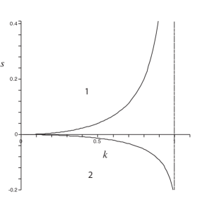
(a)

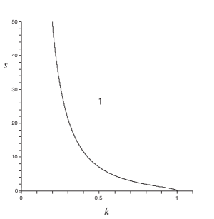
(b)

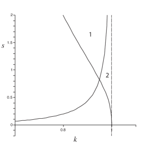
(c)

Figure 1: In (a), region 1 (resp. 2) represents the subset of the $k$-$s$ space in which the inequality (55) (resp. (56)) holds. In (b), region 1 is where the inequality in (16) for the existence of the solution of CGL holds. The curve in (b) has an asymptote at $k=0$ and its value at $k=1$ is $s=-1/4$. In (c), the top curve from (a) and the curve from (b) intersect near the point (0.949,0.824); regions 1 and 2 are explained in Figure 2

.

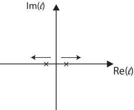
(a)

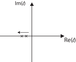
(b)

Figure 2: Diagram (a) (resp. (b)) represents the behavior of the two emerging eigenvalues for values of $k$ and $s$ in region 1 (resp. 2) of Figure 1c .

Appendix A Expressions for ${\rm\mathbf{V}}^{h}_{3}$, ${\rm\mathbf{V}}^{h}_{4}$, ${\rm\mathbf{w}}^{1}_{3}$, ${\rm\mathbf{w}}^{1}_{4}$, ${\rm\mathbf{w}}^{2}_{1}$, and ${\rm\mathbf{w}}^{2}_{2}$

The first component of ${\rm\mathbf{V}}^{h}_{3}$ is given by

$$\left({\rm\mathbf{V}}^{h}_{3}\right)_{1}=-\delta k\left[k^{\prime 2}\operatorname{dn}(\delta x)\operatorname{sn}(\delta x)\,\delta x+(2k^{2}-1)\left(\dfrac{E}{K}\delta x+Z(\delta x)\right)\right]$$

Furthermore, $\left({\rm\mathbf{V}}^{h}_{3}\right)_{2}=\left({\rm\mathbf{V}}^{h}_{3}\right)_{1}$ and $\left({\rm\mathbf{V}}^{h}_{3}\right)_{i},i=3,4$ are both given by the derivative of $\left({\rm\mathbf{V}}^{h}_{3}\right)_{1}$.

The first component of ${\rm\mathbf{V}}^{h}_{4}$ is given by

$$\left({\rm\mathbf{V}}^{h}_{4}\right)_{1}=-\dfrac{k}{k^{\prime 2}}\left[\left(\dfrac{E}{K}-k^{\prime 2}\right)\operatorname{cn}(\delta x)\,\delta x+\operatorname{cn}(\delta x)Z(\delta x)-\operatorname{dn}(\delta x)\operatorname{sn}(\delta x)\right]$$

Furthermore, $\left({\rm\mathbf{V}}^{h}_{4}\right)_{2}=-\left({\rm\mathbf{V}}^{h}_{4}\right)_{1}$ and $\left({\rm\mathbf{V}}^{h}_{4}\right)_{i},i=3,4$ are given, respectively, by the derivatives of $\left({\rm\mathbf{V}}^{h}_{4}\right)_{i},i=1,2$.

The expressions for ${\rm\mathbf{w}}^{1}_{3}$, ${\rm\mathbf{w}}^{1}_{4}$, ${\rm\mathbf{w}}^{2}_{1}$, and ${\rm\mathbf{w}}^{2}_{2}$ are rather complicated. However, for the purpose of calculating the derivatives of the Evans functions, we only need their expressions evaluated at $x=T=4K/\delta$:

$${\rm\mathbf{w}}^{1}_{3}(T)=\displaystyle{\frac{-2\mathrm{i}k\,E}{k^{\prime 2}}}\begin{bmatrix}\displaystyle{\frac{4k^{2}E}{\delta k^{\prime 2}}}\\ \\ \displaystyle{-\frac{4k^{2}E}{\delta k^{\prime 2}}}\\ \\ 1\\ \\ -1\end{bmatrix},\;\;{\rm\mathbf{w}}^{1}_{4}(T)=\displaystyle{\frac{2\mathrm{i}k\,E}{\delta k^{\prime 2}}}\begin{bmatrix}\delta^{-1}\\ \\ \delta^{-1}\\ \\ \displaystyle{\frac{4k^{2}E}{k^{\prime 2}}}\\ \\ \displaystyle{\frac{4k^{2}E}{k^{\prime 2}}}\end{bmatrix},$$

$${\rm\mathbf{w}}^{2}_{1}(T)=\displaystyle{\frac{-1}{\delta^{2}k\,k^{\prime 2}}}\begin{bmatrix}\displaystyle{E(2k^{2}-1)+Kk^{\prime 2}}\\ \\ \displaystyle{E(2k^{2}-1)+Kk^{\prime 2}}\\ \\ \displaystyle{\frac{2\delta\left(k^{\prime 4}{\it K}^{2}+2\,k^{\prime 2}\left(2\,{k}^{2}-1\right){\it E}\,{\it K}-\left(3\,{k}^{2}-4\,{k}^{4}-1\right){\it E}^{2}\right)}{k^{\prime 2}}}\\ \\ \displaystyle{\frac{2\delta\left(k^{\prime 4}{\it K}^{2}+2\,k^{\prime 2}\left(2\,{k}^{2}-1\right){\it E}\,{\it K}-\left(3\,{k}^{2}-4\,{k}^{4}-1\right){\it E}^{2}\right)}{k^{\prime 2}}}\end{bmatrix},$$

$${\rm\mathbf{w}}^{2}_{2}(T)=\displaystyle{\frac{-1}{\delta^{2}k\,k^{\prime 2}}}\begin{bmatrix}-\displaystyle{\frac{2\left(k^{\prime 4}{\it K}^{2}-2\,k^{\prime 2}{\it E}\,{\it K}+\left({k}^{2}+1\right){\it E}^{2}\right)}{\delta k^{\prime 2}}}\\ \\ \displaystyle{\frac{2\left(k^{\prime 4}{\it K}^{2}-2\,k^{\prime 2}{\it E}\,{\it K}+\left({k}^{2}+1\right){\it E}^{2}\right)}{\delta k^{\prime 2}}}\\ \\ \displaystyle{Kk^{\prime 2}-E}\\ \\ \displaystyle{-Kk^{\prime 2}+E}\end{bmatrix}.$$

Appendix B The Evans Function for Cnoidal NLS Solutions

In this appendix we use solutions of the AKNS spectral problem for focusing NLS solution

$$q_{0}(x,t)=\delta ke^{-\mathrm{i}\alpha t}\operatorname{cn}(\delta x;k),\qquad\alpha=\delta^{2}(1-2k^{2})$$ (57)

(corresponding to (3)) to construct solutions of the ODE system (8) using squared AKNS eigenfunctions. We demonstrate that for all but five values of $\ell$ along the imaginary axis (including $\ell=0$), such solutions form a basis for the solution space of (8). Using this information, we determine all zeros of the Evans function (other than possibly the four other imaginary values) using the Floquet spectrum of $q_{0}$.

B.1 Squared Eigenfunctions and the Evans Ansatz

In this subsection, we will assume that $q$ is a genus one finite-gap solution of focusing NLS (1). These solutions have the form

$$q(x,t)=e^{-\mathrm{i}\alpha t}U_{0}(\xi),\qquad\quad\xi=x-ct,$$

for real constants $\alpha,c$ and a $T$-periodic function $U_{0}$ which is not necessarily real. (We will later specialize to the case of the cnoidal solution above.) The change of variables $u_{1}(\xi,t)=e^{\mathrm{i}\alpha t}q_{1}(x,t)$, $u_{2}(\xi,t)=e^{-\mathrm{i}\alpha t}q_{2}(x,t)$ will allow us to linearize about a stationary periodic solution when it is applied to system (1), yielding

$$\mathrm{i}u_{1t}+u_{1\xi\xi}-\mathrm{i}cu_{1\xi}+\alpha u_{1}+2u_{1}^{2}u_{2} =0,$$ (58)

$$-\mathrm{i}u_{2t}+u_{2\xi\xi}+\mathrm{i}cu_{2\xi}+\alpha u_{2}+2u_{1}u_{2}^{2} =0.$$

(Note that, here, the time derivative holds $\xi$ fixed.) We linearize this system about the solution $u_{1}=\overline{u_{2}}=U_{0}(\xi)$, yielding

$$\mathrm{i}\mathrm{v}_{1t}+\mathrm{v}_{1\xi\xi}-\mathrm{i}c\mathrm{v}_{1\xi}+\alpha\mathrm{v}_{1}+4|U_{0}|^{2}\mathrm{v}_{1}+2U_{0}^{2}\mathrm{v}_{2} =0,$$ (59)

$$-\mathrm{i}\mathrm{v}_{2t}+\mathrm{v}_{2\xi\xi}+\mathrm{i}c\mathrm{v}_{2\xi}+\alpha\mathrm{v}_{2}+4|U_{0}|^{2}\mathrm{v}_{2}+2\overline{U_{0}}^{2}\mathrm{v}_{1} =0.$$

We will now show how to obtain solutions for this linearized system, satisfying the ansatz

$$\mathrm{v}_{1}=\mathrm{e}^{\ell t}w_{1}(\xi),\qquad\mathrm{v}_{2}=\mathrm{e}^{\ell t}w_{2}(\xi).$$ (60)

Recall the AKNS system for focusing NLS [2, 3]:

$$\boldsymbol{\psi}_{x}=\begin{bmatrix}-\mathrm{i}\lambda&\mathrm{i}q\\ \mathrm{i}\overline{q}&\mathrm{i}\lambda\end{bmatrix}\boldsymbol{\psi},\quad\boldsymbol{\psi}_{t}=\begin{bmatrix}\mathrm{i}(|q|^{2}-2\lambda^{2})&2\mathrm{i}\lambda q-q_{x}\\ 2\mathrm{i}\lambda\overline{q}+\overline{q_{x}}&\mathrm{i}(2\lambda^{2}-|q|^{2})\end{bmatrix}\boldsymbol{\psi}.$$ (61)

As is well known [12, 21], the squares of the components of $\boldsymbol{\psi}$ give a solution of the linearization of (1) at $q$. This linearization is

$$\mathrm{i}g_{t}+g_{xx}+4|q|^{2}g+2q^{2}h =0,$$ (62)

$$-\mathrm{i}h_{t}+h_{xx}+4|q|^{2}h+2\overline{q}^{2}g =0,$$

and the solution is given by $g=\psi_{1}^{2}$, $h=\psi_{2}^{2}$. It is easy to check that the substitutions

$$q(x,t)=\mathrm{e}^{-\mathrm{i}\alpha t}U_{0}(\xi),\quad g(x,t)=\mathrm{e}^{-\mathrm{i}\alpha t}\mathrm{v}_{1}(\xi,t),\quad h(x,t)=\mathrm{e}^{\mathrm{i}\alpha t}\mathrm{v}_{2}(\xi,t)$$ (63)

turn (62) into (59).

It is also well known that one can use Riemann theta functions to produce formulas for finite-gap solutions of NLS and the corresponding solutions of (61), starting with a hyperelliptic Riemann surface $\Sigma$ of genus $g$ and certain other data (see [3] or [5]). The solution (57) arises for $g=1$, with the four branch points of $\Sigma$ in conjugate pairs in the complex plane, so that the equation of $\Sigma$ is

$$\mu^{2}=(\lambda-\lambda_{1})(\lambda-\overline{\lambda_{1}})(\lambda-\lambda_{2})(\lambda-\overline{\lambda_{2}}),$$ (64)

where $\operatorname{\sf Re}\lambda_{1}<\operatorname{\sf Re}\lambda_{2}$. (See §3 of [5] for a derivation of these solutions from general finite-gap formulas.) In genus one, the finite-gap solutions of (61), which are known as Baker eigenfunctions, take the form

$$\psi_{1} =\exp\left(\mathrm{i}(\Omega_{1}(P)-\tfrac{E}{2})x+\mathrm{i}(\Omega_{2}(P)+\tfrac{N}{2})t\right)\Theta_{1}(\xi,P),$$

$$\psi_{2} =\exp\left(\mathrm{i}(\Omega_{1}(P)+\tfrac{E}{2})x+\mathrm{i}(\Omega_{2}(P)-\tfrac{N}{2})t\right)\Theta_{2}(\xi,P),$$

where $E,N$ are constants determined by $\Sigma$, $P=(\lambda,\mu)$ is an arbitrary point on $\Sigma$ that projects to $\lambda\in{\mathbb{C}}$, $\Omega_{1,2}$ are certain Abelian integrals on $\Sigma$, and $\Theta_{1,2}$ will be defined below. For the moment, we note that $\Theta_{1},\Theta_{2}$ depend only on $P$ and $\xi=x-ct$ (where $c$ is determined by the branch points of $\Sigma$) and are $T$-periodic in $\xi$.

After the substitutions (63) the squared Baker eigenfunctions yield solutions to (59) of the form

$$\begin{bmatrix}\mathrm{v}_{1}\\ \mathrm{v}_{2}\end{bmatrix}=\begin{bmatrix}e^{\mathrm{i}\alpha t}\psi_{1}^{2}\\ e^{-\mathrm{i}\alpha t}\psi_{2}^{2}\end{bmatrix}=e^{2\mathrm{i}\xi\Omega_{1}(P)+2\mathrm{i}t\left(\Omega_{2}(P)+c\Omega_{1}(P)\right)}\begin{bmatrix}e^{\mathrm{i}(N-cE+\alpha)t-\mathrm{i}E\xi}\Theta_{1}(\xi,P)^{2}\\ e^{\mathrm{i}(cE-N-\alpha)t+\mathrm{i}E\xi}\Theta_{2}(\xi,P)^{2}\end{bmatrix}.$$

In particular, these $\mathrm{v}_{1},\mathrm{v}_{2}$ satisfy the ansatz (60) for $\alpha=cE-N$ and

$$\ell=2\mathrm{i}(\Omega_{2}(P)+c\Omega_{1}(P)),$$ (65)

with

$$w_{1}(\xi)=e^{\mathrm{i}(2\Omega_{1}(P)-E)\xi}\Theta_{1}(\xi;P)^{2},\quad w_{2}(\xi)=e^{\mathrm{i}(2\Omega_{1}(P)+E)\xi}\Theta_{2}(\xi;P)^{2}.$$ (66)

Proposition 4.

The formula (65) implies that $\ell=4\mathrm{i}\mu$.

Proof.

The surface $\Sigma$ has genus 1, and a basis $a$ and $b$ (shown in Figure 3) for homology cycles. The differentials $\mathrm{d}\Omega_{1},\mathrm{d}\Omega_{2}$ have zero $a$-period. Denoting their $b$-periods as $V,W$ respectively, from [5] we have

$$W/V=-c=(\lambda_{1}+\lambda_{2}+\overline{\lambda_{1}}+\overline{\lambda_{2}}).$$

(Note that the meaning of $c$ here is $-1$ times its definition in [5].) Thus, the differential

$$\mathrm{d}\ell=2\mathrm{i}(\mathrm{d}\Omega_{2}+c\,\mathrm{d}\Omega_{1})$$

has zero $a$- and $b$-periods. So, although $\Omega_{1,2}$ are not well-defined on $\Sigma$, and so $\ell$ is a well-defined function on $\Sigma$.

The integrals $\Omega_{i}$ use the branchpoint $\overline{\lambda_{2}}$ as basepoint, so $\ell=0$ there. Because $\iota^{*}\mathrm{d}\Omega_{i}=-\mathrm{d}\Omega_{i}$ for $i=1,2$ (where $\iota$ is the sheet exchange automorphism $(\lambda,\mu)\mapsto(\lambda,-\mu)$), then $\iota^{*}\ell=-\ell$. So, it follows that $\ell$ vanishes at all four branch points, which are the same points at which the coordinate $\mu$ vanishes. The surface $\Sigma$ has two points at infinity, called $\infty_{\pm}$, where both $\lambda$ and $\mu$ approach complex infinity and

$$\dfrac{\mu}{\lambda^{g+1}}=\dfrac{\mu}{\lambda^{2}}=\pm\left(1+\dfrac{c}{2}\lambda^{-1}+{\mathcal{O}}(\lambda^{-2})\right)$$

respectively. Combining the asymptotic expansions for $\Omega_{1}$ and $\Omega_{2}$ gives

$$\dfrac{\ell}{\lambda^{2}}=\pm 2\mathrm{i}\left(2+c\lambda^{-1}+{\mathcal{O}}(\lambda^{-2})\right).$$

Therefore,

$$\ell/\mu=4\mathrm{i}+{\mathcal{O}}(\lambda^{-2}).$$

Because $\ell/\mu$ is bounded and holomorphic on $\Sigma$, then it must be equal to the constant $4\mathrm{i}$, i.e.,

$$\ell=4\mathrm{i}\mu.$$

In other words, we have just proved the identity

$$\Omega_{2}(P)=-c\Omega_{1}(P)+2\mu$$ (67)

for genus one NLS solutions. ∎

B.2 Forming a Basis of Solutions

Proposition 4 and (64) imply that for generic values of $\ell$ there are four distinct points $P\in\Sigma$ for which the Baker eigenfunctions may be used to construct a solution of the eigenvalue problem (6). The exceptional values are those for which two roots of (64), as a polynomial equation for $\lambda$, coincide.

From here on, we specialize to the case where the branch points in (64) satisfy $\lambda_{2}=-\overline{\lambda_{1}}$, with $\operatorname{\sf Re}\lambda_{1}\neq 0$, which yields the NLS solution (57). In this case, $c=0$ and $E=V/2$, the branch points are related to the elliptic modulus by $\lambda_{1}/|\lambda_{1}|=-k^{\prime}+\mathrm{i}k$, and the finite-gap solution coincides with (57) with $\delta=2|\lambda_{1}|$. The exceptional values of $\mu$ are

$$\mu=\pm|\lambda_{1}|^{2},\qquad\mu=\pm\operatorname{\sf Im}(\lambda_{1}^{2}),$$ (68)

corresponding respectively to a double root occurring at $\lambda=0$, or two pairs of roots coinciding at opposite points along the real axis (if $k^{2}<1/2$) or imaginary axis (if $k^{2}>1/2$).

When $\mu$ is not an exceptional value, we will construct a matrix solution $W(\xi;\ell)$ of (8) where each column is of the form $[w_{1}(\xi),w_{2}(\xi),w_{1}^{\prime}(\xi),w_{2}^{\prime}(\xi)]^{T}$ and $w_{1},w_{2}$ are given by (66) for one of the four points $P=(\lambda,\mu)$ satisfying (64) for the given $\mu$. For purposes of showing that the matrix solution is nonsingular, it suffices to evaluate its determinant at one value of $\xi$.

We now need to specify the form of the factors $\Theta_{1},\Theta_{2}$ in (66). Specializing the formulas given in §5 of [5], and using $\xi=x-ct=x$, we have

$$\Theta_{1}(x;P)=\dfrac{\theta(A(P)+\mathrm{i}Vx-D)\theta(D)}{\theta(\mathrm{i}Vx-D)\theta(A(P)-D)},\quad\Theta_{2}(x;P)=-\mathrm{i}e^{\Omega_{3}(P)}\dfrac{\theta(A(P)+\mathrm{i}Vx-D-R)\theta(D)}{\theta(\mathrm{i}Vx-D)\theta(A(P)-D)}.$$

In these formulas,

• $V=\pi|\lambda_{1}-\overline{\lambda_{2}}|/K=2\pi|\lambda_{1}|/K$;

• $A(P)$ is the Abel map, obtained by integrating the differential $\omega=V\,\mathrm{d}\lambda/(2\mu)$ from $\infty_{-}$ to $P$ on $\Sigma$;

• $\Omega_{3}(P)$ is the integral, from $\overline{\lambda_{2}}$ to $P$, of the unique meromorphic differential $\mathrm{d}\Omega_{3}$ on $P$ which has zero $a$-period and satisfies $\mathrm{d}\lambda_{1}\sim\pm\lambda^{-1}\mathrm{d}\lambda$ near $\infty_{\pm}$;

• $R$ is minus the period of $\mathrm{d}\Omega_{3}$ on the cycle $b$ running from $\lambda_{1}$ to $\lambda_{2}$ (see Figure 3), and is also the value $A(\infty_{+})$, when the path of integration is chosen to avoid the homology cycles $a$ and $b$ (see §5 in [5]); in the case when $c=0$, $R=\pi(K^{\prime}/K+\mathrm{i})$ (see §3 in [5]);

• $D$ is an arbitrary constant which is pure imaginary;

• $\theta(z)$ is the Riemann theta function with period $2\pi\mathrm{i}$ and quasiperiod $B=-2\pi K^{\prime}/K$. It is related to the Jacobi theta functions of modulus $k$ by $\theta(z)=\theta_{3}(z/(2\mathrm{i}))$.

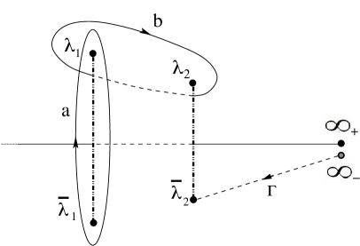
Figure 3: Homology cycles and other integration paths on the genus one Riemann surface with complex conjugate branch points. Solid curves appear on the upper sheet, dashed curves on the lower sheet, and branch cuts extend between each branch point and its conjugate. The horizontal line represents a set of points where $\mu$ is real and positive.

In genus one, the constant $D$ has no significance, as it can be absorbed through a shift in $x$. Thus, we may assume $D=0$ in the above formulas. Once this is done, the columns of $W$ for $\xi=0$ take the form

$$\begin{bmatrix}w_{1}(0)\\ w_{2}(0)\\ w_{1}^{\prime}(0)\\ w_{2}^{\prime}(0)\end{bmatrix}=\begin{bmatrix}1\\ -f(P)^{2}\\ 2\mathrm{i}g(P)\\ -2\mathrm{i}f(P)^{2}h(P)\end{bmatrix},$$ (69)

where

$$f(P):=e^{\Omega_{3}(P)}\dfrac{\theta(A(P)-r)}{\theta(A(P))},\quad g(P):=\Omega_{1}(P)+V\Theta(A(P))-\frac{E}{2},\\ h(P):=\Omega_{1}(P)+V\Theta(A(P)-r)+\frac{E}{2},\hskip 227.62204pt$$

and $\Theta(z)=\theta^{\prime}(z)/\theta(z)$ is the logarithmic derivative of the Riemann theta function. (Note that $A(P)$ and $\Omega_{i}(P)$ are not individually well-defined on $\Sigma$, because of the nonzero periods of the corresponding differentials along the homology cycles. We take the convention that the paths of integration for these differ by a fixed path $\Gamma$ (shown in Figure 3) from $\infty_{-}$ to $\overline{\lambda_{2}}$ in $\Sigma_{0}$, where $\Sigma_{0}$ denotes the simply-connected domain that results from cutting $\Sigma$ along the homology cycles. With this convention, $f,g,h$ are well-defined meromorphic functions on $\Sigma$.)

The Riemann surface $\Sigma$ has two holomorphic involutions, namely $\iota:(\lambda,\mu)\mapsto(\lambda,-\mu)$ and $\sigma:(\lambda,\mu)\mapsto(-\lambda,\mu)$. Because $\iota^{*}\mathrm{d}\Omega_{i}=-\mathrm{d}\Omega_{i}$, $\iota^{*}\omega=-\omega$ and $\iota$ fixes the basepoint for $\Omega_{i}$, $i=1,2,3$, it follows that

$$f(\iota P)=1/f(P),\qquad g(\iota P)=-h(P).$$

Because $\sigma^{*}\mathrm{d}\Omega_{1}=-\mathrm{d}\Omega_{1}$, $\sigma^{*}\mathrm{d}\Omega_{3}=\mathrm{d}\Omega_{3}-\omega$, $\sigma^{*}\omega=-\omega$, and $E=V/2$, it follows that

$$f(\sigma P)=f(P),\qquad g(\sigma P)=-g(P).$$

Let $P_{1},P_{2},P_{3},P_{4}$ be four points on $\Sigma$ corresponding to a given (non-exceptional) value of $\mu$. Without loss of generality, we may assume that $P_{2}=\sigma(P_{1})$ and $P_{4}=\sigma(P_{3})$. Using the above formulas for the behaviour of $f,g,h$ under $\sigma$, we find that the matrix with columns given by (69) is

$$W(0)=\begin{bmatrix}1&1&1&1\\ -f(P_{1})^{2}&-f(P_{1})^{2}&-f(P_{3})^{2}&-f(P_{3})^{2}\\ 2\mathrm{i}g(P_{1})&-2\mathrm{i}g(P_{1})&2\mathrm{i}g(P_{3})&-2\mathrm{i}g(P_{3})\\ -2\mathrm{i}f(P_{1})^{2}h(P_{1})&2\mathrm{i}f(P_{1})^{2}h(P_{1})&-2\mathrm{i}f(P_{3})^{2}h(P_{3})&2\mathrm{i}f(P_{3})^{2}h(P_{3})\end{bmatrix}.$$

Proposition 5.

The functions $g,h$ satisfy the identity

$$-g(P)=h(P)=\lambda,\qquad P=(\lambda,\mu)\in\Sigma.$$

Proof.

The poles of $g(P)=\Omega_{1}(P)+\Theta(A(P))-E/2$ can only occur where $\Omega_{1}$ has a pole or $\theta(A(P))=0$. (We now work on the cut Riemann surface $\Sigma_{0}$.) These occur only at $\infty_{-}$ (near which $\Omega_{1}\sim-\lambda+{\mathcal{O}}(1)$, but $\theta(A(P))=\theta(0)=\sqrt{2K/\pi}\neq 0$), and at $\infty_{+}$ (near which $\Omega_{1}\sim\lambda+{\mathcal{O}}(1)$ and $\theta(A(P))=\theta(R)=0$). Near $\infty_{+}$, use $w=\lambda^{-1}$ as local coordinate. Then $A(P)=\tfrac{V}{2}\int_{\infty_{-}}^{P}\mu^{-1}\mathrm{d}\lambda$ implies that

$$\dfrac{\mathrm{d}A(P)}{\mathrm{d}w}=-\dfrac{V}{2w^{2}\mu}=-\dfrac{V}{2}(1+{\mathcal{O}}(w^{2}))$$

and therefore $A(P)=R-\tfrac{V}{2}w+{\mathcal{O}}(w^{3})$. Because $\theta(z)$ has a simple zero at $z=R$,

$$g(P)=\Omega_{1}(P)+V\dfrac{\theta^{\prime}(A(P))}{\theta(A(P))}-\frac{E}{2}=w^{-1}+V\left(\dfrac{-2}{V}\right)w^{-1}+{\mathcal{O}}(1)=-\lambda+{\mathcal{O}}(1).$$

The oddness of $g$ with respect to $\sigma$ implies that $g(P)=0$ when $P$ lies over the origin in the $\lambda$-plane. Therefore, the quotient $g(P)/\lambda$ is a bounded holomorphic function on $\Sigma$, and so must be a constant. The above asymptotic expansion for $g$ implies that $g(P)=-\lambda$, and it follows from the fact that $h(\iota P)=-g(P)$ that $h(P)=\lambda$. ∎

Taking Prop. 5 into account, we compute

$$\det W(0)=-16\lambda(P_{1})\lambda(P_{3})(f(P_{1})^{2}-f(P_{3})^{2})^{2}.$$ (70)

Proposition 6.

For $\mu$ not equal to zero or any of the exceptional values in (68), the matrix $N$ is nonsingular. (We conjecture that the analogous statement is true for genus one finite-gap solutions in general.)

Proof.

Because we are excluding the exceptional values, neither of the $\lambda$-values in (70) are zero, and it only remains to establish that $f(P_{1})\neq\pm f(P_{3})$.

Define $F(P)=f(P)+1/f(P)$, which is a well-defined meromorphic function of $\lambda$. The formula for $f(P)$ shows that its only pole is a second-order pole at $\infty_{+}$ (because $\exp(\Omega_{3}(P))\sim\lambda$ near there), and hence $F$ is a second-order polynomial in $\lambda$. It is known that $f(\pm\lambda_{1})=1$ and $f(\pm\overline{\lambda_{1}})=-1$ (see §7 of [6]). Hence,

$$F(\lambda)=\dfrac{4(\lambda^{2}-d)}{\lambda_{1}^{2}-\overline{\lambda_{1}}^{2}},\qquad d:=\operatorname{\sf Re}(\lambda_{1}^{2}).$$

Using the quadratic formula, and the fact that $f$ has a second-order zero at $\infty_{-}$, we obtain

$$f(P)=\dfrac{2(\lambda^{2}-d+\mu)}{\lambda_{1}^{2}-\overline{\lambda_{1}}^{2}}.$$ (71)

Let $y_{1}=\lambda(P_{1})$ and $y_{3}=\lambda(P_{3})$. Because $y_{1}$ and $y_{3}$ are distinct roots of

$$(\lambda^{2}-\lambda_{1}^{2})(\lambda^{2}-\overline{\lambda_{1}}^{2})=\mu^{2},$$ (72)

and $y_{1}\neq-y_{3}$, then $y_{1}^{2}+y_{3}^{2}=2d$. Hence, $F(y_{1})=2(y_{1}^{2}-y_{3}^{2})=-F(y_{3})$, and therefore $f(P_{1})\neq f(P_{3})$. Furthermore, using (71), we see that

$$(\lambda_{1}^{2}-\overline{\lambda_{1}}^{2})(f(P_{1})+f(P_{3}))=2(y_{1}^{2}+y_{3}^{2}-2d+2\mu)=4\mu.$$

Thus, because we assume $\mu\neq 0$, $f(P_{1})\neq-f(P_{3})$. ∎

Assuming that $\mu$ is not zero or one of the exceptional values, we can define the transfer matrix

$$N=W(T)W(0)^{-1},$$

whose eigenvalues describe the growth of solutions to (8) over one period. (In particular, there is a periodic solution if and only if $N$ has eigenvalue one.) Using the fact that $T=4\pi/V=2\pi/E$ and $\Omega_{1}(\sigma\,P)=-\Omega_{1}(P)+E/2$ on the cut surface, we calculate that

$$W(T)=W(0)\begin{bmatrix}e^{2\mathrm{i}\Omega_{1}(P_{1})T}&0&0&0\\ 0&e^{-2\mathrm{i}\Omega_{1}(P_{1})T}&0&0\\ 0&0&e^{2\mathrm{i}\Omega_{1}(P_{3})T}&0\\ 0&0&0&e^{-2\mathrm{i}\Omega_{1}(P_{3})T}\end{bmatrix}.$$

Then the characteristic polynomial of the transfer matrix is

$$\det(N-\tau I)=((\tau+1)^{2}-4\tau\cos(\Omega_{1}(P)T))((\tau+1)^{2}-4\tau\cos(\Omega_{1}(P_{3})T)).$$

By substituting $\tau=1$ in this formula, we obtain the

Proposition 7.

For $\mu$ not equal to zero or the exceptional values in (68), the system (8), where $\ell=4\mathrm{i}\mu$, has a periodic solution if and only if $\sin(\Omega_{1}(P_{1})T)=0$ or $\sin(\Omega_{1}(P_{3})T)=0$.

B.3 Imaginary Zeros of the Evans Function

For periodic finite-gap solutions of NLS, the Floquet discriminant [5] takes the form

$$\Delta(\lambda)=2\cos\left(\dfrac{2\pi}{V}\Omega_{1}(P)\right)=2\cos\left(\dfrac{T}{2}\Omega_{1}(P)\right).$$

(While $\Omega_{1}$ is odd with respect to the involution $\iota$, the even-ness of the cosine makes $\Delta$ a well-defined function of $\lambda$.) This has the property that the AKNS system (61) admits a T-periodic (respectively, antiperiodic) solution if and only $\Delta=\pm 2$.

The consequence of Propositions 6 and 7 is that, for values of $\ell$ that correspond to nonzero values of $\mu$ excluding those in (68), the Evans function is equal to zero if and only if $\Delta=\pm 2$ or $\Delta=0$ at an opposite pair out of the four $\lambda$-values corresponding to $\mu$. When this happens, the corresponding pair of columns of $W$ are periodic, and the corresponding value of $\ell$ is a zero of the Evans function of geometric multiplicity two. Thus, we can use the Floquet discriminant to find the (nonexceptional) zeros of the Evans function.

In §3.5 of [5], the discriminant for genus one finite-gap solutions is calculated as

$$\Delta(\lambda)=-2\cos\left[2\mathrm{i}K\left(Z(u)-\beta^{2}\dfrac{\operatorname{cn}u\operatorname{dn}u\operatorname{sn}u}{1-\beta^{2}\operatorname{sn}^{2}u}\right)\right],$$ (73)

where the variable $u$ is related to $\lambda$ by

$$\operatorname{sn}^{2}u=\varphi(\lambda):=\dfrac{(\lambda_{1}-\overline{\lambda}_{2})(\lambda-\overline{\lambda}_{1})}{(\lambda_{1}-\overline{\lambda}_{1})(\lambda-\overline{\lambda}_{2})}$$ (74)

and the parameter $\beta$ and the modulus $k$ are related to the branch points by

$$k^{2}=\dfrac{-(\lambda_{1}-\overline{\lambda}_{1})(\lambda_{2}-\overline{\lambda}_{2})}{|\lambda_{1}-\overline{\lambda}_{2}|^{2}},\quad\beta^{2}=\dfrac{\lambda_{1}-\overline{\lambda}_{1}}{\lambda_{1}-\overline{\lambda}_{2}}.$$

In the symmetric case (i.e., $\lambda_{2}=-\overline{\lambda}_{1}$) which we are considering here, these specialize to

$$-k^{\prime}+\mathrm{i}k=\lambda_{1}/|\lambda_{1}|,\qquad\beta^{2}=k(k-\mathrm{i}k^{\prime}),$$

and the variable $u$ is determined by $\lambda$ as follows. The function $\operatorname{sn}^{2}u$ has periods $2K$ and $2\mathrm{i}K^{\prime}$, and is even in $u$, so it suffices to restrict $u$ to the set $(0,K]\times(-K^{\prime},K^{\prime}]$ in the complex plane. Then there is a unique $u$ in this set for each $\lambda$ in the extended complex plane. Conversely, solving (74) for $\lambda$ in terms of $u$ gives

$$\lambda(u)=\dfrac{\lambda_{1}\operatorname{sn}^{2}u+\overline{\lambda}_{1}\beta^{-2}}{\beta^{-2}-\operatorname{sn}^{2}u}.$$

The locus of $\lambda$-values for which $\Delta(\lambda)$ is real and between $2$ and $-2$ is known as the continuous Floquet spectrum of the NLS potential $q$. For genus one solutions, it consists of the real axis and two bands terminating at the branch points. (For low values of $k$ the bands emerge from the real axis, but for $k$ sufficiently near 1, the bands become detached from the real axis (see Figure 4); the transition occurs around $k\simeq.9089$ [14].)

The periodic points (i.e., where $\Delta=\pm 2$) consist of the branch points and countably many points (known as double points) on the real axis. Points where $\Delta=0$ will naturally interlace the periodic points along the real axis, but will also occur along the imaginary axis if the bands are detached. When this happens, though, the corresponding value of $\mu$ is real. Hence, all the zeros of the Evans function will occur along the imaginary axis in the complex $\ell$-plane.

Figures 4 and 5 show the level sets of $\Delta(\lambda)$ for several different moduli, and the zeros of Evans function in the $\ell$-plane. The latter figures also include the locus of $\ell$-values which are related by (72), with $\ell=4\mathrm{i}\mu$, to $\lambda$-values in the continuous spectrum.

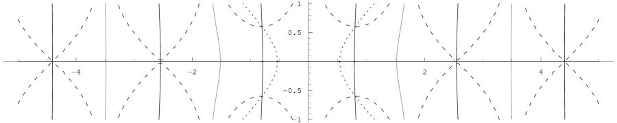
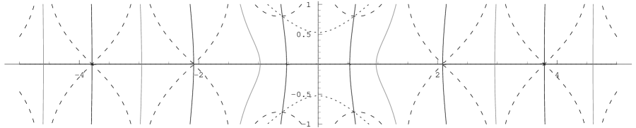
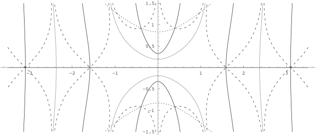
Figure 4: Level curves of the Floquet discriminant $\Delta$ in the complex $\lambda$-plane for elliptic moduli $k=.6$, $k=.8$ and $k=.92$, respectively. (We take $|\lambda_{1}|=\delta/2=1$.) In each of the diagrams, the black curves indicate where $\Delta$ is real, the gray curves where $\Delta$ is imaginary, the dashed curves where $\operatorname{\sf Re}\Delta=\pm 2$, and the dotted curves where $\mu$ is real (which includes the real and imaginary axes). Thus, branch points occur where dotted intersects dashed, periodic points occur where black intersects dashed, and points where $\Delta=0$ occur where black intersects grey.

Figure 5: Zeros of the Evans function in the complex $\ell$-plane, for $k=.6$, $k=.8$ and $k=.92$, respectively. Note that all zeros are of multiplicity two, except for the origin, which is of multiplicity four. The continuous spectrum consists of the imaginary axis and the figure eight curve.

References

- [1] G. P. Agrawal, Optical pulse propagation in doped fiber amplifiers, Phys. Rev. A 44, 7493–7501 (1991).
- [2] M.J. Ablowitz, D.J. Kaup, A.C. Newell and H. Segur, The inverse scattering transform – Fourier analysis for nonlinear problems, Stud. Appl. Math. 53 (1974), 249–315.
- [3] E. Belokolos, A. Bobenko, A. B. V. Enolskii , A. Its, and V. Matveev, Algebro-Geometric Approach to Nonlinear Integrable Equations, Springer, 1994.
- [4] P. Byrd and M. Friedman, Handbook of Elliptic Integrals for Engineers and Physicists (2nd ed.), Springer, 1971.
- [5] A. Calini and T. Ivey, Finite-gap Solutions of the Vortex Filament Equation: Genus One Solutions and Symmetric Solutions, J. Nonlinear Sci. 15 (2005), 321–361.
- [6] –, Finite-gap Solutions of the Vortex Filament Equation: Isoperiodic Deformations, submitted to J. Nonlinear Science.
- [7] J. D. Carter and B. Deconinck, Instabilities of one-dimensional trivial-phase solutions of the two-dimensional cubic nonlinear Schr dinger equation, Phys. D 214 (2006), 42–54.
- [8] G. Cruz-Pacheco, C. D. Levermore, and B. P. Luce, Complex Ginzburg-Landau as perturbations of nonlinear Shrödinger equations: a case study, preprint.
- [9] G. Cruz-Pacheco, C. D. Levermore, and B. P. Luce, Complex Ginzburg-Landau as perturbations of nonlinear Shrödinger equations: a Melnikov approach, Phys. D 197, 269-285 (2004).
- [10] G. Cruz-Pacheco, C. D. Levermore, and B. P. Luce, Complex Ginzburg-Landau as perturbations of nonlinear Shrödinger equations: traveling wave persistence, preprint.
- [11] N. Ercolani, M. G. Forest, and D. W. McLaughlin, Geometry of the modulational instability III. Homoclinic orbits for the periodic sine-Gordon equation, Phys. D 43 (1990), 349–384.
- [12] M. G. Forest and J. E. Lee, Geometry and modulation theory for the periodic nonlinear Schrödinger equation. Oscillation theory, computation, and methods of compensated compactness, IMA Vol. Math. Appl. 2 (1986)., 35–69
- [13] R. A. Gardner, Spectral analysis of long wavelength periodic waves and applications, J. Reine Angew. Math. 491 (1997)., 149–181
- [14] T. Ivey and D. Singer, Knot types, homotopies and stability of closed elastic rods, Proc. London Math. Soc. 79 (1999), 429–450.
- [15] T. Kapitula and B. Sandstede, Stability of bright solitary-wave solutions to perturbed nonlinear Schrödinger equations, Phys. D 124 (1998)., 58–103
- [16] T. Kapitula and J. Rubin, Existence and stability of standing hole solutions to complex Ginzburg-Landau equations, Nonlinearity 13 (2000), 77-112.
- [17] P. Kolodner, Drift, shape, and intrinsic destabilization of pulses of traveling-wave convection, Phys. Rev. A 44 (1991)., 6448–6465
- [18] Y. Kuramoto, Chemical oscillations, waves and turbulence, Springer-Verlag (1984).
- [19] J. Lega and S. Fauve, Traveling hole solutions to the complex Ginzburg-Landau equation as perturbations of nonlinear Schrödinger dark solitons, Phys. D 102 (1997), 234–252.
- [20] Y. Li and D. W.McLaughin, Morse and Melnikov functions for NLS Pde’s, Commun. Math. Phys. 162 (1994), 175-214.
- [21] D. W.McLaughin and E. A. Overman II, Whiskered Tori for Integrable Pde’s: Chaotic Behavior in Integrable Pde’s, pp. 83–203 in Surveys in Applied Mathematics 1, Plenum Press, 1995.
- [22] A. C. Newell and J. A. Whithead, Finite bandwidth, finite amplitude convection, J. Fluid Mech. 38 (1969), 279–303.