A new approach to resummation: Parametric Perturbation Theory

Abstract

We present a non–perturbative method, called Parametric Perturbation Theory (PPT), which is alternative to the ordinary perturbation theory. The method relies on a principle of simplicity for the observable solutions, which are constrained to be linear in a certain (unphysical) parameter. The perturbative expansion is carried out in this parameter and not in the physical coupling (as in ordinary perturbation theory). We show that the method is capable to resum the divergent perturbative series, to extract the leading asymptotic (strong coupling) behavior and predict with high accuracy the coefficients of the perturbative series.

In this letter we present a method, called Parametric Perturbation Theory (PPT), which can be used to resum series, either divergent or with a finite radius of convergence, which appear in the perturbative solution of physical problems. The approach behind our method is completely new and it is based on few simple ideas: the first idea, which we call Principle of Absolute Simplicity (PAS), is that, instead of expanding the observable (energy, frequency, $\dots$) in the physical coupling $g$, and thus obtain to a finite order a polynomial in $g$, we impose that the observable has the simplest possible form (linear) in a given unphysical parameter $\varrho$; the second idea is that the expansion must be carried out in $\varrho$ and that the functional relation $g=g(\varrho)$ (unknown) must comply with the PAS to the order to which the calculation is done. This will allow to determine the relation between $g$ and $\rho$ and in turn to obtain the observable as a parametric function of $\varrho$.

Consider for example a model which depends on a parameter $g$, and which is solvable when $g=0$. Clearly, the application of Perturbation Theory (PT) to the calculation of a physical observable $\mathcal{O}$ to a finite order yields a polynomial in $g$. Calling $r$ the radius of convergence of the perturbative series, the direct use of PT must be restricted to $|g|<r$. However, the misbehavior of the perturbative series for $\mathcal{O}$ is the result of having expanded in a parameter, $g$, which is not optimal. As a matter of fact, if one knew the exact solution to the problem, i.e. $\mathcal{O}=f(g)$, then this solution could be considered as a polynomial of order one in the variable $\varrho=f(g)$. Although this observation by itself cannot be used as a constructive principle, we may adopt the philosophy that the perturbative series for the observable can be simpler and convergent in all the domain, if it is cast in terms of a suitable parameter $\varrho$. Only if such parameter, by luck or ability, turns out to be the $\varrho=f(g)$ discussed above, the exact solution is obtained. The goal, therefore, is to progressively build this parameter $\varrho$ to yield an expression for $\mathcal{O}$ as simple as possible. In this framework the perturbative expansion is carried out in $\varrho$ and all the physical quantities in the problem are expressed as functions of $\varrho$. In particular we have now that $g=g(\varrho)$. While the ordinary perturbation theory works by calculating the contributions to higher orders in $g$, each term of higher order refining the result to lower order, the approach approach is the opposite: we carry out a perturbative calculation in $\varrho$, and then determine order by order the form of $g=g(\varrho)$ so that the observable $\mathcal{O}(\varrho)$ can be a order one polynomial in $\varrho$, as required by the Principle of Absolute Simplicity.

Although in this letter we focus on the implementation of this method as a technique for resumming perturbative series, we show in a companion and more detailed paper that the same philosophy can be used to obtain a perturbation scheme fully autonomous from perturbation theory.

Let us first sketch briefly how the method works and then apply it to some non-trivial perturbative series. Consider an observable $\mathcal{O}$, represented through the perturbative series perturbatively to some order

$$\mathcal{O}^{(PT)}=\sum_{n=0}^{N}b_{n}\ g^{n}\ ,$$ (1)

where $N=\infty$ in some cases. The series could be either convergent, with a finite radius of convergence, or divergent, although we will not worry at this time. The full implementation of the method requires the introduction of an unphysical parameter, $\varrho$, and the specification of a functional relation between $g$ and $\varrho$:

$$g=g(\varrho)\ .$$ (2)

The choice of this relation is not completely arbitrary, since it must be capable of reproducing the perturbative terms when expanded around $g=0$. For example, in many of the cases which we have studied we have used

$$g(\varrho)=\varrho\ \left[\frac{1+\sum_{n=1}^{\bar{N}_{u}}c_{n}\varrho^{n}}{1+\sum_{n=1}^{\bar{N}_{d}}d_{n}\varrho^{n}}\right],$$ (3)

where the coefficients $c_{n}$ and $d_{n}$ are unknown to be determined applying the PAS. $\bar{N}_{u}$ and $\bar{N}_{d}$ are integers.

The Principle of Absolute Simplicity requires that the observable be linear in $\varrho$, i.e.

$$\mathcal{O}^{(PPT)}=b_{0}+b_{1}\varrho\ .$$ (4)

If we substitute eq. (3) inside eq. (1) and expand around $\varrho=0$, working to a given order specified by the sum $\bar{N}_{u}+\bar{N}_{d}=\bar{N}$, then we can fully determine the coefficients $c_{n}$ and $d_{n}$ by requiring that an equal number of nonlinear terms in $\varrho$ vanish, starting with the term going as $\varrho^{2}$. Notice that the choice of the integer parameters $\bar{N}_{u}$ and $\bar{N}_{d}$ determines the asymptotic behavior of $g$ as $\varrho\rightarrow\infty$ (we are assuming for simplicity that the denominator in (3) never vanish for $\varrho>0$):

$$g(\varrho)\approx\varrho^{\bar{N}_{u}-\bar{N}_{d}+1}$$ (5)

and in turn

$$\mathcal{O}^{(PPT)}\approx b_{0}+b_{1}g^{1/(\bar{N}_{u}-\bar{N}_{d}+1)}\ .$$ (6)

Therefore in cases where the asymptotic behavior is known, one can choose $\bar{N}_{u}$ and $\bar{N}_{d}$ to reproduce the exact asymptotic behavior of the solution; on the other hand, when the asymptotic behavior is unknown, working to a given order $\bar{N}_{u}+\bar{N}_{d}=\bar{N}$, one can select the most appropiate asympotic behavior among those allowed by the combination of $\bar{N}_{u}$ and $\bar{N}_{d}$ which keep $\bar{N}$ fixed.

We will first apply the method to a model of $\phi^{4}$ field theory in zero dimensions JZJ , which will allow us to discuss some other properties of our resummation. We consider the integral

$$E(g)=\int_{0}^{+\infty}e^{-x^{2}-gx^{4}}dx\ ,$$ (7)

whose perturbative series is divergent. Eq.(7) admits an exact analytical solution given by

$$E(g)=\frac{e^{\frac{1}{8g}}}{4\sqrt{g}}\ K_{1/4}\left(\frac{1}{8g}\right)\ ,$$ (8)

where $K_{1/4}(g)$ is the Bessel function of order $1/4$. Notice that for negative values of $g$ this expression acquires an imaginary part, signaling that the system becomes metastable.

We will now analyze this problem with the help of PPT, using a slightly different functional relation than the one in eq. (3):

$$g(\varrho)=\varrho\ \left[\frac{1+\sum_{n=1}^{\bar{N}}c_{n}\varrho^{n}}{1+\sum_{n=1}^{\bar{N}+1}d_{n}\varrho^{n}}\right]^{5}.$$ (9)

Notice that this relation implements the correct asymptotic behavior, $E(g)\propto g^{-1/4}$ as $g\rightarrow\infty$.

Using $\bar{N}=3$ we have found the transformation:

$$g(\varrho)\approx\frac{\rho\left(2925\varrho^{3}+881.8\varrho^{2}+58.8\varrho+1\right)^{5}}{\left(-1737.2\varrho^{4}+2243.9\varrho^{3}+832.2\varrho^{2}+58\varrho+1\right)^{5}}\ .$$ (10)

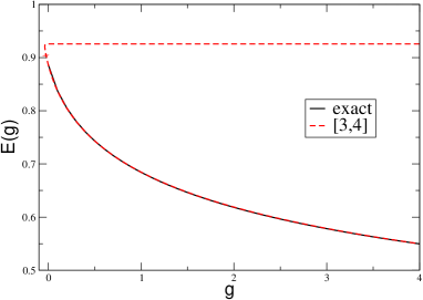
Figure 1: (color online) Comparison between the set $[3,4]$ and the exact integral. The approximate solution has a branch point close to $g=0$.

Since $\varrho_{0}=-0.0593$ is a zero of the denominator, $\lim_{\varrho\rightarrow\varrho_{0}}g(\varrho)=\infty$: this result signals the presence of a branch point in the proximity of $\varrho_{0}$ (see Fig.1). The existence of this branch point can be understood as a signal of the no-analyticity of the exact solution in $g=0$, which is the reason why the perturbative series diverges.

In the region $g<0$ the analytic continuation of the solution acquires an imaginary part. Using eq.(10) we find the numerical solutions of $g(\varrho)=g$, with $g<0$. For example, corresponding to $g=-1$ we obtain two pairs of complex conjugated roots accompanied by a single real root:

$$\varrho_{1} = 0.20784+0.54897\ i$$ (11)

$$\varrho_{2} = 0.20784-0.54897\ i$$ (12)

$$\varrho_{3} = -0.24838$$ (13)

$$\varrho_{4} = -0.22321+0.00636i$$ (14)

$$\varrho_{5} = -0.22321-0.00636i\ .$$ (15)

Obtaining a complex value for $\varrho$ has an immediate effect on the observable $E(g)$, which acquires an imaginary part, $ImE(g)=b_{1}\ Im\varrho$. Therefore we can verify if one of these solutions corresponds to the exact solution of (7) for $g=-1$:

$$ImE(g)=-0.37679$$ (16)

which should be compared to the imaginary parts calculated with the PPT using the numerical roots $\varrho_{i}$, $i=1,\dots,5$:

$$ImE(g)^{PPT}_{1} = -0.36488$$ (17)

$$ImE(g)^{PPT}_{2} = 0.364886$$ (18)

$$ImE(g)^{PPT}_{3} = 0$$ (19)

$$ImE(g)^{PPT}_{4} = -0.00422$$ (20)

$$ImE(g)^{PPT}_{5} = 0.00422\ .$$ (21)

The comparison between exact and approximate real and imaginary parts of the integral for negative $g$ is shown in Fig.2.

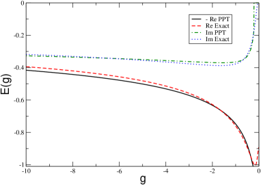
Figure 2: (color online) Real and imaginary parts of $E(g)$ for the zero dimensional $\phi^{4}$ theory obtained using the PPT with $\bar{N}=3$. The results are compared with the exact expression of eq.(7).

These results suggest that the first root corresponds to the analytic continuation of the solution for $g>0$ to negative values. On the other hand the real part of $ReE(g)^{PPT}_{1}=0.74808$ has the opposite sign of $ReE(g)=-0.76033$: this happens because our function is continous and therefore it is not possible to reproduce a discontinuity at $g=0$. The exponential behavior of the exact solution for $g\rightarrow 0^{-}$ cannot be reproduced in this approach.

We will now discuss a different problem, a lattice $\phi^{4}$ model in $1+1$ dimensions, described by the hamiltonian Nish01

$$\hat{H}=\sum_{i}\left[\frac{1}{2}\hat{\pi}_{i}^{2}+\hat{\phi}_{i}^{4}+g\left(\frac{1}{2}\left(\hat{\phi}_{i}-\hat{\phi}_{i+1}\right)^{2}+\frac{1}{2}\hat{\phi}_{i}^{2}\right)\right]\ ,$$ (22)

where $i$ is the site index and $\hat{\pi}_{i}$ and $\hat{\phi}_{i}$ are canonically conjugated operators.

Nishiyama has studied this model using both a linked cluster expansion, calculating the perturbative contributions to order $g^{11}$, and the Density Matrix Renormalization Group (DMRG). Since the perturbative series has a radius of convergence $g_{0}\approx 1$, he used an Aitken $\delta^{2}$ process to accelerate the convergence of this series, obtaining moderately improved results. Using these results, he speculated the existence of a singularity corresponding to $g\approx-2$ (using our notation) and of a Ising-type phase transition for a critical negative $g$.

We can apply PPT to this problem using eq.(3) and considering the sets corresponding to $\bar{N}=5$. Comparing the difference $E(g)^{PT}-E(g)^{PPT}$ we have found that the optimal set corresponds to $[\bar{N}_{u},\bar{N}_{d}]=[3,2]$. In Table 1 we compare the exact perturbative coefficients going from $b_{7}$ to $b_{11}$ as given in Nish01 with those predicted by the set $[3,2]$. The largest error corresponds to $b_{11}$ and is of just $0.1\%$!

Table 1: Comparison between the perturbative coefficients of Nish01 and those predicted with PPT working with the set $[3,2]$.

	$b_{7}$	$b_{8}$	$b_{9}$	$b_{10}$	$b_{11}$
$b_{n}^{exact}$	0.01106139	-0.00874935	0.00709675	-0.00587143	0.00493622
$b_{n}^{[3,2]}$	0.01106113	-0.00874838	0.00709460	-0.00586767	0.00493037
error ($\%$)	0.00233	0.011081739435	0.03022	0.06403	0.11851

Figure 3: (color online) Comparison between the resummed energies to orders $[3,2]$, $[4,3]$ and $[5,4]$ and the perturbative polynomials.

In Fig.3 we have compared the perturbative polynomials for the energy from orders $g^{2}$ to $g^{11}$ with the energy resummed with the sets $[3,2]$, $[4,3]$ and $[5,4]$. There are several striking aspects which should impress the reader: first of all, the difference between the three sets is extremely thin, thus signaling that the convergence is extremely strong; in second place, the resummed energy confirms the DMRG result displayed in Fig.2 of Nish01 ; finally, the resummed energy is a multivalued function, with a branch point at $g\approx-1.025$, falling extremely close to the singularity speculated by Nishiyama . Because of the use of a parameter $\varrho$, PPT can deal with multivalued functions in a way which is not possible in conventional perturbation theory. Finally, the thiny dashed line in the plot corresponds to the numerical result obtained in Amore06a using the Variational Sinc Collocation Method (VSCM) within a mean field approach.

As a last example, we apply PPT to the prediction of virial coefficients of a hard sphere gas in $D=2,3$ dimensions. Ref.Clis06 contains the values for the first $10$ virial coefficients for $D=2,\dots,8$. In this case, we have found out that the optimal choice corresponds to $\bar{N}_{u}=\bar{N}_{d}-1$, thus implying (using our notation) that $\lim_{\varrho\rightarrow\infty}g(\varrho)=\bar{g}<\infty$, i.e. that the resummed function will have a singularity precisely at $g=\bar{g}$.

Working with the set $[3,4]$ we have found

$$\bar{g}^{[3,4]}_{D=2}\approx 1.1625\ \ ,\ \ \bar{g}^{[3,4]}_{D=3}\approx 1.43439\ .$$ (23)

In Table 2 we have considered the different sets corresponding to $\bar{N}_{u}+\bar{N}_{d}=5$, which use the first eigth virial coefficients as input, and used them to predict $B_{9}$ and $B_{10}$, which have already been calculated Clis06 . The error (in percent) of the prediction of $B_{9}$ with the set $[2,3]$ is of about $0.035\%$ and $0.54\%$ in $D=2$ and $D=3$ respectively.

Table 2: Virial coefficients for a hard spheres in $2$ and $3$ dimensions given in Table I of Clis06 and predictions using PPT with different sets.

	$B_{9}/B_{2}^{8}$	$B_{10}/B_{2}^{9}$	$B_{9}/B_{2}^{8}$	$B_{10}/B_{2}^{9}$
	$D=2$		$D=3$
Ref.Clis06	$0.0362193$	$0.0199537$	$0.0013094$	$0.0004035$
$[0,5]$	$0.03739998$	$0.02496595$	$0.0023400$	$0.0031580$
$[1,4]$	$0.03625994$	$0.02008503$	$0.0013509$	$0.0004884$
$[2,3]$	$0.0362321$	$0.0199843$	$0.0013165$	$0.0004198$
$[3,2]$	$0.0362551$	$0.02006717$	$0.0013404$	$0.0004664$
$[4,1]$	$0.0368599$	$0.02258546$	$0.0017325$	$0.0014442$
$[5,0]$	$0.1747048$	$0.75984885$	$0.0222648$	$0.0735264$

In Table 3 we have compared our predictions for the virial coefficients $B_{11}$ through $B_{18}$ using PPT with the set $[3,4]$ with the predictions made in Clis06 , finding very similar results for $D=2$ but rather different results in the case $D=3$.

Table 3: Predicted coefficients for approximants with 10 exact coefficients for $D=2$ and $D=3$. Comparison between the predictions of Clis06 and the predictions obtained using the set $[3,4]$.

	$B_{11}/B_{2}^{10}$	$B_{12}/B_{2}^{11}$	$B_{13}/B_{2}^{12}$	$B_{14}/B_{2}^{13}$	$B_{15}/B_{2}^{14}$	$B_{16}/B_{2}^{15}$	$B_{17}/B_{2}^{16}$	$B_{18}/B_{2}^{17}$
$D=2$
Ref.Clis06	$1.089\times 10^{-2}$	$5.90\times 10^{-3}$	$3.18\times 10^{-3}$	$1.70\times 10^{-3}$	$9.10\times 10^{-4}$	$4.84\times 10^{-4}$	$2.56\times 10^{-4}$	$1.36\times 10^{-4}$
$[3,4]$	$1.0901\times 10^{-2}$	$5.9235\times 10^{-3}$	$3.2117\times 10^{-3}$	$1.7421\times 10^{-3}$	$9.4698\times 10^{-4}$	$5.1638\times 10^{-4}$	$2.8247\times 10^{-4}$	$1.5492\times 10^{-4}$
$D=3$
Ref.Clis06	$1.22\times 10^{-4}$	$3.64\times 10^{-5}$	$1.08\times 10^{-5}$	$3.2\times 10^{-6}$	$9.2\times 10^{-7}$	$2.6\times 10^{-7}$
$[3,4]$	$1.1599\times 10^{-4}$	$2.2229\times 10^{-5}$	$-8.5616\times 10^{-6}$	$-1.8088\times 10^{-5}$	$-2.0325\times 10^{-5}$	$-2.0112\times 10^{-5}$	$-1.9136\times 10^{-5}$	$-1.7971\times 10^{-5}$

Concluding, our method has several interesting features: it can describe multivalued functions, it can provide the imaginary part of the observable corresponding to a metastable state, it can resum divergent series and select the most appropriate asymptotic behavior of the solution among those available at a given order. Finally, it can also be used to make accurate predictions of yet unknown perturbative coefficients. Further applications of this method have been considered in a lengthier and more detailed paper.

References

- (1) C.M.Bender and E.J.Weniger, J. Math. Phys.42, 2167-2183 (2001)
- (2) J.Zinn-Justin, Quantum Field Theory and Critical Phenomena, Clerendon Press-Oxford, New York (2002); I.R.C.Buckley, A. Duncan and H.F.Jones, Phys.Rev.D 47, 2554-2559 (1993); C.M.Bender, A. Duncan and H.F.Jones, Phys.Rev.D 49, 4219-4225
- (3) Y. Nishiyama, J.Phys.A 34, 11215-11223 (2001)
- (4) P.Amore, J.Phys.A L349-L355 (2006)
- (5) N.Clisby and B. McCoy, Jour. of Stat. Phys. 122 15-57 (2006)