Path Integral Methods in the Su-Schrieffer-Heeger Polaron Problem

Summary I propose a path integral description of the Su-Schrieffer-Heeger Hamiltonian, both in one and two dimensions, after mapping the real space model onto the time scale. While the lattice degrees of freedom are classical functions of time and are integrated out exactly, the electron particle paths are treated quantum mechanically. The method accounts for the variable range of the electronic hopping processes. The free energy of the system and its temperature derivatives are computed by summing at any $T$ over the ensemble of relevant particle paths which mainly contribute to the total partition function. In the low $T$ regime, the heat capacity over T ratio shows un upturn peculiar to a glass-like behavior. This feature is more sizeable in the square lattice than in the linear chain as the overall hopping potential contribution to the total action is larger in higher dimensionality. The effects of the electron-phonon anharmonic interactions on the phonon subsystem are studied by the path integral cumulant expansion method.

1 Introduction

There has been a growing interest towards polarons over recent years also in view of the technological potential of polymers, organic molecules friend ; capasso ; nasu ; dallak ; krish ; han ; brat , carbon nanotubes veri and high $T_{c}$ superconductors alex in which polaronic properties, essentially dependent on the type and strength of the electron-phonon coupling alekor ; aletv ; i1 , have been widely discussed.

One dimensional (1D) systems with a half filled band undergo a structural distortion peierls which increases the elastic energy and opens a gap at the Fermi surface thus lowering the electronic energy. The competition between lattice and electronic subsystems stabilizes the 1D structure which accordingly acquires semiconducting properties whereas the behavior of the 3D system would be metallic-like.

Conjugated polymers, for example polyacetylene, show anisotropic electrical and optical properties lu due to intrinsic delocalization of $\pi$ electrons along the chain of CH units. As the intrachain bonding between adjacent CH monomers is much stronger than the interchain coupling the lattice is quasi-1D. Hence, as a result of the Peierls instability, trans-polyacetylene shows an alternation of short and long neighboring carbon bonds, a dimerization, accompanied by a two fold degenerate ground state energy. Charge injection in polymers induces a lattice distortion with the associated formation of localized excitations, polarons and/or charged solitons. While the latter can exist only in trans-polyacetylene, the former solutions are more general since they do not require such degeneracy.

The Su-Schrieffer-Heeger (SSH) model Hamiltonian ssh has become a successful tool in polymer physics as it hosts the peculiar ground state excitations of the 1D conjugated structure and it accounts for a broad range of polymer properties macdiarmid ; cat ; ssh1 . In the weak coupling regime a continuum version tlm of the SSH model has been developed and polaronic solutions have been obtained analytically campbell . Although the 1D properties of the SSH model have been mainly investigated so far schulz ; fradkin ; stafstrom ; raedt ; zheng ; pucci ; capone ; i2 , extensions to two dimensions were considered in the late eighties in connection with the Fermi surface nesting effect on quasi 2D high $T_{c}$ superconductors tang . Recent numerical analysis ono have revealed the rich physics of 2D-SSH polarons whose mass seems to be larger than in the 1D case, at least in the intermediate regime of the adiabatic parameter i3 .

As a fundamental feature of the SSH Hamiltonian the electronic hopping integral linearly depends on the relative displacement between adjacent atomic sites thus leading to a nonlocal e-ph coupling sto ; per with vertex function depending both on the electronic and the phononic wave vector. The latter property induces, in the Matsubara formalism mahan , an electron hopping associated with a time dependent lattice displacement. As a consequence time retarded electron-phonon interactions arise in the system yielding a source current which depends both on time and on the electron path coordinates. This causes large e-ph anharmonicities in the equilibrium thermodynamics of the SSH model i4 . Hopping of electrons from site to site accompanied by a coupling to the lattice vibration modes is a fundamental process determining the transport lang and equilibrium properties of many body systems nieu . A variable range hopping may introduce some degree of disorder thus affecting the charge mobility fish ; plyuk and the thermodynamic functions.

These issues are hereafter analyzed by means of the path integral formalism feynman ; devreese ; farias ; ganbold ; raedt1 ; korn which fully accounts for the time retarded e-ph interactions as a retarded potential naturally emerges in the exact integral action kleinert . Using the main property of the e-ph coupling model, the Hamiltonian linearly dependent on the phonon displacement field, I attack the SSH model after introducing a generalized version of the semiclassical model which treats only the electrons quantum mechanically. Being valid for any e-ph coupling value, the path integral method allows one to derive the partition function and the related temperature derivatives without those limitations which affect the perturbative studies. The general formalism, both for the 1D and 2D system, is described in Section 2 while the path integral approach used to derive the full partition function of the interacting system is developed in Section 3. In Section 4, I outline the main features of the computational method and derive the thermodynamical properties for a particle described by a SSH Hamiltonian in a bath of harmonic oscillators. In Section 5, the model is generalized in order to include the electron-phonon effects on the oscillator bath: the anharmonic corrections to the total heat capacity are evaluated by a path integral cumulant expansion in terms of the source current of the Hamiltonian model. Some conclusions are drawn in Section 6.

2 The Hamiltonian Model

In a square lattice with isotropic nearest neighbors hopping integral $J$, the SSH Hamiltonian for electrons plus e-ph interactions reads:

$$H=\, \sum_{r,s}\Bigl{[}(J_{r,s})_{x}\bigl{(}f^{{\dagger}}_{r+1,s}f_{r,s}+h.c.\bigr{)}\,$$

$$+ (J_{r,s})_{y}\bigl{(}f^{{\dagger}}_{r,s+1}f_{r,s}+h.c.\bigr{)}\Bigr{]}\,$$

$$(J_{r,s})_{x}=\, -{1\over 2}\bigl{[}J+\alpha\Delta u_{x}\bigr{]}\,$$

$$(J_{r,s})_{y}=\, -{1\over 2}\bigl{[}J+\alpha\Delta u_{y}\bigr{]}\,$$

$$\Delta u_{x}=\, u_{x}(r+1,s)-{u_{x}(r,s)}\,$$

$$\Delta u_{y}=\, u_{y}(r,s+1)-{u_{y}(r,s)}\quad,\,$$

where $\alpha$ is the electron-phonon coupling, ${\bf u}(r,s)$ is the dimerization coordinate indicating the displacement of the monomer group on the $(r,s)-$ lattice site, $f^{{\dagger}}_{r,s}$ and $f_{r,s}$ create and destroy electrons (i.e., $\pi$ band electrons in polyacetylene). The phonon Hamiltonian is given by a set of 2D classical harmonic oscillators. The two addenda in Eq. (LABEL:eq:1) deal with one dimensional e-ph couplings along the x and y axis respectively, with first neighbors electron hopping. Second neighbors hopping processes (with overlap integral $J^{(2)}$) may be accounted for by adding to the Hamiltonian the term $H^{(2)}$ such that

$$H^{(2)}=\,(J_{r,s})_{x,y}\bigl{(}f^{{\dagger}}_{r+1,s+1}f_{r,s}+h.c.\bigr{)}\,$$

$$(J_{r,s})_{x,y}=\,-{1\over 2}\Bigl{[}J^{(2)}+\alpha\sqrt{(\Delta u_{x})^{2}+(\Delta u_{y})^{2}}\Bigr{]}\quad.\,$$

(2)

The 1D SSH Hamiltonian is obtained by Eq. (LABEL:eq:1) just dropping the second term depending on the $y$ coordinate. The real space Hamiltonian in Eq. (LABEL:eq:1) can be transformed into a time dependent Hamiltonian hamann by introducing the electron coordinates: i) $\bigl{(}x(\tau^{\prime}),y(\tau^{\prime})\bigr{)}$ at the $(r,s)$ lattice site, ii) $\bigl{(}x(\tau),y(\tau^{\prime})\bigr{)}$ at the $(r+1,s)$ lattice site and iii) $\bigl{(}x(\tau^{\prime}),y(\tau)\bigr{)}$ at the $(r,s+1)$ lattice site, respectively. $\tau$ and $\tau^{\prime}$ vary on the scale of the inverse temperature $\beta$. The spatial e-ph correlations contained in Eq. (LABEL:eq:1) are mapped onto the time axis by changing: $u_{x,(y)}(r,s)\to u_{x,(y)}(\tau^{\prime})$, $u_{x}(r+1,s)\to u_{x}(\tau)$ and $u_{y}(r,s+1)\to u_{y}(\tau)$. Now we set $\tau^{\prime}=\,0$, $\bigl{(}x(\tau^{\prime}),y(\tau^{\prime})\bigr{)}\equiv(0,0)$, $\bigl{(}u_{x}(\tau^{\prime}),u_{y}(\tau^{\prime})\bigr{)}\equiv(0,0)$. Accordingly, Eq. (LABEL:eq:1) transforms into the time dependent Hamiltonian:

$$H(\tau) = \,J_{x}(\tau)\Bigl{(}f^{{\dagger}}(x(\tau),0)f(0,0)+h.c.\Bigr{)}\,$$

$$+ J_{y}(\tau)\Bigl{(}f^{{\dagger}}(0,y(\tau))f(0,0)+h.c.\Bigr{)}\,$$

$$J_{x}(\tau) = \,-{1\over 2}\bigl{[}J+\alpha u_{x}(\tau)\bigr{]}\,$$

$$J_{y}(\tau) = \,-{1\over 2}\bigl{[}J+\alpha u_{y}(\tau)\bigr{]}\quad.\,$$

While the ground state of the 1D SSH Hamiltonian is twofold degenerate, the degree of phase degeneracy is believed to be much higher in 2D ono1 as many lattice distortion modes contribute to open the gap at the Fermi surface. However, as in 1D, these phases are connected by localized and nonlinear excitations, the soliton solutions. Thus, also in 2D both electron hopping between solitons kivel and thermal excitation of electrons to band states may take place within the model. These features are accounted for by the time dependent version of the Hamiltonian. As $\tau$ varies continuously on the $\beta$ scale and the $\tau$-dependent displacement fields are continuous variables (whose amplitudes are in principle unbound in the path integral), long range hopping processes are automatically included in $H(\tau)$ which is therefore more general than the real space SSH Hamiltonian in Eq. (LABEL:eq:1) (and Eq. (2)). Thus, by means of the path integral formalism we look at the low temperature thermodynamical behavior both in 1D and 2D searching for those features which may be ascribable to some local disorder related to the variable range of the hopping processes.

The semiclassical nature of the model is evident from Eq. (LABEL:eq:3) in which quantum mechanical degrees of freedom interact with the classical variables $u_{x(y)}(\tau)$. Averaging the electron operators over the ground state we obtain the time dependent semiclassical energy per lattice site $N$ which is linear in the atomic displacements:

$${{<H(\tau)>}\over N}=\,J_{x}(\tau)P\bigl{(}J,\tau,x(\tau)\bigr{)}+J_{y}(\tau)P\bigl{(}J,\tau,y(\tau)\bigr{)}\,$$

$$P\bigl{(}J,\tau,{\bf v}(\tau)\bigr{)}=\,{1\over{\pi^{2}}}\int d{\bf k}\cos[{\bf k\cdot v}(\tau)]\cosh(\epsilon_{\bf k}\tau)n_{F}(\epsilon_{\bf k})\quad,\,$$

(4)

with ${\bf v}(\tau)=\,(x(\tau),0)$ and ${\bf v}(\tau)=\,(0,y(\tau))$ in the first and second term respectively. $\epsilon_{\bf k}=\,-J\sum_{i=x,y}\cos(k_{i})$ is the electron dispersion relation and $n_{F}$ is the Fermi function. The chemical potential has been pinned to the zero energy level. Eq. (4) can be rewritten in a way suitable to the path integral approach by defining

$${{<H(\tau)>}\over N}=\,V\bigl{(}{x}(\tau)\bigr{)}+V\bigl{(}{y}(\tau)\bigr{)}+{\bf u}(\tau)\cdot{\bf j}({\bf v}(\tau))\,$$

$$V\bigl{(}{x}(\tau)\bigr{)}=\,-JP\bigl{(}J,\tau,{x}(\tau)\bigr{)}\,$$

$$V\bigl{(}{y}(\tau)\bigr{)}=\,-JP\bigl{(}J,\tau,{y}(\tau)\bigr{)}\,$$

$${\bf j}({\bf v}(\tau))=-\alpha P\bigl{(}J,\tau,{\bf v}(\tau)\bigr{)}\,$$

$${\bf u}(\tau)=\,\bigl{(}u_{x}(\tau),u_{y}(\tau)\bigr{)}\quad.\,$$

(5)

$V\bigl{(}{x}(\tau)\bigr{)}$ and $V\bigl{(}y(\tau)\bigr{)}$ are the effective terms accounting for the $\tau$ dependent electronic hopping while ${\bf j}({\bf v}(\tau))$ is interpreted as the external source kleinert current for the oscillator field ${\bf u}(\tau)$. Averaging the electrons over the ground state we neglect the fermion-fermion correlations hirsch which lead to effective polaron-polaron interactions in non perturbative analysis of the model acqua . This approximation however is not expected to affect substantially the following calculations.

3 The Path Integral Formalism

Taking a bath of $\bar{N}$ 2D oscillators, we write the SSH electron path integral, ${\bf\zeta}(\tau)\equiv\,\bigl{(}{x}(\tau),{y}(\tau)\bigr{)}$, as:

$$<{\bf\zeta}(\beta) | {\bf\zeta}(0)>=\,\prod_{i=1}^{\bar{N}}\int D{\bf u}_{i}(\tau)\int D{\bf\zeta}(\tau)\,$$

$$\cdot exp\Biggl{[}-\int_{0}^{\beta}d\tau\sum_{i=1}^{\bar{N}}{M\over 2}\biggl{(}\dot{\bf u}_{i}^{2}(\tau)+\omega_{i}^{2}{\bf u}_{i}^{2}(\tau)\biggr{)}\Biggr{]}\,$$

$$\cdot exp\Biggl{[}-\int_{0}^{\beta}d\tau\biggl{(}{m\over 2}\dot{\bf\zeta}^{2}(\tau)+V\bigl{(}{x}(\tau)\bigr{)}+V\bigl{(}{y}(\tau)\bigr{)}\biggr{)}\,$$

$$+ \sum_{i=1}^{\bar{N}}{\bf u}_{i}(\tau)\cdot{\bf j}({\bf v}(\tau))\Biggr{]}\quad,\,$$

where $m$ is the electron mass, $M$ is the atomic mass and $\omega_{i}$ is the oscillator frequency. As a main feature we notice that the interacting energy is linear in the atomic displacement field. Then, the electronic path integral can be derived after integrating out the oscillator degrees of freedom which are decoupled along the $x$ and $y$ axis. Accordingly, we get:

$$<{\bf\zeta}(\beta)|{\bf\zeta}(0)>=\,\prod_{i=1}^{\bar{N}}Z_{i}\Biggl{[}\int D{x}(\tau)\,$$

$$\cdot exp\Bigl{[}-\int_{0}^{\beta}d\tau\biggl{(}{m\over 2}\dot{x}^{2}(\tau)+V\bigl{(}{x}(\tau)\bigr{)}\biggr{)}-{1\over\hbar}A({x}(\tau))\Bigr{]}\Biggr{]}^{2},\,$$

$$A({x}(\tau))=\,-{{\hbar^{2}}\over{4M}}\sum_{i=1}^{\bar{N}}{1\over{\hbar\omega_{i}\sinh(\hbar\omega_{i}\beta/2)}}\,$$

$$\cdot \int_{0}^{\beta}d\tau j({x}(\tau))\int_{0}^{\beta}d{\tau^{\prime\prime}}\cosh\Bigl{(}\hbar\omega_{i}\bigl{(}|\tau-{\tau^{\prime\prime}}|-\beta/2\bigr{)}\Bigr{)}j({x}({\tau^{\prime\prime}})),\,$$

$$Z_{i}=\,\Bigl{[}{1\over{2\sinh(\hbar\omega_{i}\beta/2)}}\Bigr{]}^{2}\quad.\,$$

Thus, the 2D electron path integral is obtained after squaring the sum over one dimensional electron paths. This permits to reduce the computational problem which is nonetheless highly time consuming particularly in the low temperature limit. Note in fact that the source current $j({x}(\tau))$ requires integration over the 2D Brillouin Zone (BZ) according to Eqs. (4), (5) and this occurs for any choice of the electron path coordinates. The quadratic (in the coupling $\alpha$) source action $A({x}(\tau))$ is time retarded as the particle moving through the lattice drags the excitations of the oscillator fields which take a time to readjust to the electron motion. When the interaction is sufficiently strong the conditions for polaron formation may be fulfilled in the system according to the degree of adiabaticity brown . However the present path integral description is valid independently of the existence of polarons as it applies also to the weak coupling regime. Assuming periodic conditions ${x}(\tau)=\,{x}(\tau+\beta)$, the particle paths can be expanded in Fourier components

$${x}(\tau)=\,{x}_{o}+\sum_{n=1}^{\infty}2\Bigl{(}\Re{x}_{n}\cos(\omega_{n}\tau)-\Im{x}_{n}\sin(\omega_{n}\tau)\Bigr{)}\,$$

$$\omega_{n}=\,2\pi n/\beta$$ (8)

and the open ends integral over the paths $\int D{x}(\tau)$ transforms into the measure of integration $\oint D{x}(\tau)$. Taking:

$$\oint D{x}(\tau)\equiv\int_{-\infty}^{\infty}{{d{x}_{o}}\over{\bigl{(}2\pi\hbar^{2}/mK_{B}T\bigr{)}^{(1/2)}}}\prod_{n=1}^{\infty}\Biggl{[}{{\int_{-\infty}^{\infty}d\Re{x}_{n}\int_{-\infty}^{\infty}d\Im{x}_{n}}\over{\bigl{(}\pi\hbar^{2}K_{B}T/m\omega_{n}^{2}\bigr{)}}}\Biggr{]}\quad,$$ (9)

we proceed to integrate Eq. (LABEL:eq:7) in order to derive the full partition function of the system versus temperature.

Let’s point out that, by mapping the electronic hopping motion onto the time scale, a continuum version of the interacting Hamiltonian (Eq. (LABEL:eq:3)) has been de facto introduced. Unlike previous lu approaches however, our path integral method is not constrained to the weak e-ph coupling regime and it can be applied to any range of physical parameters.

4 Computational Method and Thermodynamical Results

As a preliminar step we determine, for a given path and at a given temperature: i) the minimum number ($N_{\bf k}$) of ${\bf k}-$points in the BZ to accurately estimate the average interacting energy per lattice site and, ii) the minimum number ($N_{\tau}$) of points in the double time integration to get a numerically stable source action in Eq. (LABEL:eq:7). The momentum integrations required by Eq. (4) converge by summing over 1600 and 70 points in the reduced 2D and 1D BZ, respectively. Moreover, $N_{\tau}=\,300$ at $T=1K$.

Computation of Eqs. (4) -  (LABEL:eq:7) requires fixing two sets of input parameters. The first set contains the physical quantities characterizing the system: the bare hopping integral $J$, the oscillator frequencies $\omega_{i}$ and the effective coupling $\chi=\,\alpha^{2}\hbar^{2}/M$ (in units $meV^{3}$). The second set defines the paths for the particle motion which mainly contribute to the partition function through: the number of pairs ($\Re x_{n},\Im x_{n}$) in the Fourier expansion of Eq. (8), the cutoff ($\Lambda$) on the integration range of the expansion coefficients in Eq. (9) and the related number of points ($N_{\Lambda}$) in the measure of integration which ensures numerical convergence.

After introducing a dimensionless path

$$x(\tau)/a=\,{\bar{x}_{o}}+\sum_{n=1}^{N_{p}}\Bigl{(}\bar{a}_{n}\cos(\omega_{n}\tau)+\bar{b}_{n}\sin(\omega_{n}\tau)\Bigr{)}\quad,$$ (10)

with: $\bar{x}_{o}\equiv x_{o}/a$, $\bar{a}_{n}\equiv 2\Re x_{n}/a$ and $\bar{b}_{n}\equiv-2\Im x_{n}/a$, the functional measure of Eq. (9) can be rewritten for computational purposes as:

$$\oint Dx (\tau)\approx{a\over{\sqrt{2}}}\biggl{(}{a\over 2}\biggr{)}^{2N_{p}}{{(2\pi\cdot 4\pi\cdot\cdot\cdot 2N_{p}\pi)^{2}}\over{(\pi\hbar^{2}/mK_{B}T)^{N_{p}+1/2}}}\int_{-\Lambda/a}^{\Lambda/a}{d\bar{x}_{o}}\cdot\,$$

$$\int_{-2\Lambda/a}^{2\Lambda/a}{d\bar{a}_{1}}\int_{-2\Lambda/a}^{2\Lambda/a}{d\bar{b}_{1}}\cdot\cdot\cdot\int_{-2\Lambda/a}^{2\Lambda/a}{d\bar{a}_{N_{p}}}\int_{-2\Lambda/a}^{2\Lambda/a}{d\bar{b}_{N_{p}}}\quad.\,$$

In the following we take the lattice constant $a=\,1\AA$. As a criterion to set the cutoff $\Lambda$ on the integration range, we notice that the functional measure normalizes the kinetic term in Eq. (LABEL:eq:7):

$$\oint Dx(\tau)exp\Bigl{[}-{m\over 2}\int_{0}^{\beta}d\tau\dot{x}^{2}(\tau)\Bigr{]}\equiv 1$$ (12)

and this condition holds for any number of pairs $N_{p}$ truncating the Fourier expansion in Eq. (9). Then, taking $N_{p}=\,1$, the left hand side of Eq. (12) transforms as:

$$\oint Dx(\tau)exp\Bigl{[}-{m\over 2}\int_{0}^{\beta}d\tau\dot{x}^{2}(\tau)\Bigr{]}\simeq{4\over\pi}\Bigl{[}\int_{0}^{U}dyexp(-y^{2})\Bigr{]}^{2}\,$$

$$U\equiv\sqrt{2\pi^{3}}{\Lambda\over\lambda}\,$$

$$\lambda=\,\sqrt{{2\pi\hbar^{2}}\over{mK_{B}T}}\quad.$$ (13)

Using the series representation grad

$$\int_{0}^{U}dyexp(-y^{2})=\,\sum_{k=0}^{\infty}{{(-1)^{k}U^{2k+1}}\over{k!(2k+1)}}\quad,$$ (14)

one determines $U$ (after setting the series cutoff $k_{max}$ which ensures convergence) by fitting the Poisson integral value $\sqrt{\pi}/2$.

Thus, we find that the cutoff $\Lambda$ can be expressed in terms of the thermal wavelength $\lambda$ as $\Lambda\sim\lambda/\sqrt{2\pi^{3}}$ hence, it scales versus temperature as $\Lambda\propto 1/\sqrt{T}$. This means physically that, at low temperatures, $\Lambda$ is large since many paths are required to yield the correct normalization. For example, at $T=\,1K$, we get $\Lambda\sim 284\AA$. Numerical investigation of Eq. (LABEL:eq:7) shows however that a much shorter cutoff suffices to guarantee convergence in the path integral, while the cutoff temperature dependence implied by Eq. (12) holds also in the computation of the interacting partition function. The thermodynamical results hereafter presented have been obtained by taking $\Lambda\sim\lambda/(10\sqrt{2\pi^{3}})$. Summing in the 1D system over $N_{\Lambda}\sim 20/\sqrt{T}$ points for each integration range and taking $N_{p}=\,2$, we are then evaluating the contribution of $(N_{\Lambda}+1)^{2N_{p}+1}$ paths (the integer part of $N_{\Lambda}$ is obviously selected at any temperature). Thus, at $T=\,1K$ and in 1D, we are considering $\sim 4\cdot 10^{6}$ different paths for the particle motion while, at $T=\,100K$ the number of paths drops to 243 i5 . In the 2D problem, $N_{\Lambda}\sim 35/\sqrt{T}$ points for each Fourier coefficient are required i6 . Computation of the second order derivatives of the free energy in the range $T\in[1,301]K$, with a spacing of 3K, takes 55hours and 15 minutes on a Pentium 4. Note that larger $N_{p}$ in the path Fourier expansion would further increase the computing time without introducing any substantial improvement in the thermodynamical output of our calculation.

Although the history of the SSH model is mainly related to wide band polymers, we take here a narrow band system ($J=\,100meV$) i2 with the caveat that electron-electron correlations may become relevant in narrow bands.

Free energy and heat capacity have been first computed up to room temperature, both in 1D and 2D, assuming a bath of $\bar{N}=\,10$ low energy oscillators separated by $2meV$: $\hbar\omega_{1}=\,2meV,...,\hbar\omega_{10}=\,20meV$. The lowest energy oscillator yields the largest contribution to the phonon partition function mainly in the low temperature regime while the $\omega_{10}$ oscillator essentially sets the phonon energy scale which determines the size of the e-ph coupling. A larger number $\bar{N}$ of oscillators in the aforegiven range would not significantly modify the calculation whereas lower $\omega_{i}$ values would yield a larger contribution to the phonon partition function mainly at low $T$.

In the discrete SSH model, the value $\bar{\alpha}\equiv\,4\alpha^{2}/(\pi\kappa J)\sim 1$, marks the crossover between weak and strong e-ph coupling, with $\kappa$ being the effective spring constant. In our continuum and semiclassical model the effective coupling is $\chi$. Although in principle, discrete and continuum models may feature non coincident crossover parameters, we assume that the relation between $\alpha$ and $J$ obtained by the discrete model crossover condition still holds in our model. Hence, at the crossover we get: $\chi_{c}\sim\,\pi J\hbar^{2}\omega^{2}_{10}/64$. This means that, in Figures 1-3, the crossover value is set at $\chi_{c}\sim\,2000meV^{3}$.

In Fig.1, a comparison between the 1D and the 2D free energies is presented for two values of $\chi$, one lying in the weak and one in the strong e-ph coupling regime. The oscillator free energies $F_{ph}$ are plotted separately while the free energies arising from the total action in Eq. (LABEL:eq:7), shortly termed $F_{source}$, results from the competition between the free path action (kinetic term plus hopping potential in the exponential integrand) and the source action depending on the e-ph coupling. While the former enhances the free energy, the latter becomes dominant at increasing temperatures thus reducing the total free energy. In general, the 2D free energies have a larger gradient (versus temperature) than the corresponding 1D terms. The $F_{ph}$ lie above the $F_{source}$ both in 1D and 2D because of the choice of the $\hbar\omega_{i}$: in general one may expect a crossing point between $F_{ph}$ and $F_{source}$ with temperature location depending on the value of $\chi$. Note that the $F_{source}$ plots have a positive temperature derivative in the low temperature regime and this feature is more pronounced in 2D. In fact, at low $T$, the source action is dominated by the hopping potential $V\bigl{(}x(\tau)\bigr{)}$ while, at increasing $T$, the e-ph effects become progressively more important (as the bifurcation between the $\chi_{1}$ and $\chi_{2}$ curves shows) and the $F_{source}$ get a negative derivative. In 2D, the weight of the $V\bigl{(}x(\tau)\bigr{)}$ term is larger because there is a higher hopping probability. This physical expectation is taken into account by the path integral method. At any temperature, we monitor the ensamble of relevant particle paths over which the hopping potential is evaluated. For a selected set of Fourier components in Eq. (10) the hopping decreases by lowering $T$ but its value is still significant at low $T$. Considered that: i) the total action is obtained after a $d\tau$ integration of $V\bigl{(}x(\tau)\bigr{)}$ and ii) the $d\tau$ integration range is larger at lower temperatures, we explain why the overall hopping potential contribution to the total action is responsible for the anomalous free energy behavior at low T.

In Fig.2, the heat capacity contributions due to the oscillators ($C_{ph}$) and electrons plus e-ph coupling ($C_{sou}$) are reported on. The values are normalized over $\bar{N}$. the previously described summation over a large number of paths turns out to be essential to recover the correct thermodynamical behavior in the zero temperature limit. The dimensionality effects are seen to be large and, for a given dimensionality, the role of the e-ph interactions is magnified at increasing $T$. The total heat capacity ($C_{ph}$ + $C_{sou}$) over $T$ ratios are plotted in Fig.3 in the low $T$ regime to emphasize the presence of an anomalous upturn which appears at $T\preceq 10K$ in 1D and $T\preceq 20K$ in 2D. This feature in the heat capacity linear coefficient is ultimately related to the sizable effective hopping integral term $V\bigl{(}x(\tau)\bigr{)}$. The strength of the e-ph coupling has a minor role in the low $T$ limit although it determines the shape of the anomaly versus $T$.

Let’s focus now on the 1D system and consider the effect of the oscillators bath on the thermodynamical properties: in Figures 4-6 the ten phonon energies are: $\hbar\omega_{1}=\,22meV,...,\hbar\omega_{10}=\,40meV$. Accordingly the crossover is set at $\chi_{c}\sim\,8000meV^{3}$ and three plots out of five lie in the strong e-ph coupling regime. As shown in Fig.4, large $\chi$ values are required to get strongly decreasing free energies versus temperature while the $\chi=\,3000meV^{3}$ curve now hardly intersects the phonon free energy at room temperature. Fig.5 shows the rapid growth of the source heat capacity versus temperature at strong couplings whereas the presence of the low $T$ upturn in the total heat capacity over T ratio is confirmed in Fig.6. Note that, due to the enhanced oscillators energies, the phonon heat capacity saturates here at $T\sim 400K$ (in Fig.2, for the 1D case, $T\sim 200K$).

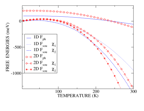
Figure 1: Phonon ($F_{ph}$) and Source Term ($F_{sou}$) contributions to the 1D and 2D free energies for two values of the effective coupling $\chi$: $\chi_{1}=\,1440meV^{3}$ (weak e-ph coupling) $\chi_{2}=\,2560meV^{3}$ (strong e-ph coupling). A bath of ten phonon oscillators is considered, the largest phonon energy being $\hbar\omega_{10}=\,20meV$.

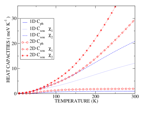
Figure 2: Phonon and Source Term contributions (normalized over the number of oscillators) to the 1D and 2D heat capacities for the same parameters as in Fig.1. The oscillator heat capacities are also plotted.

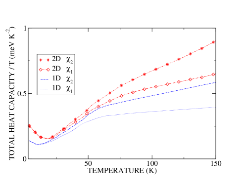
Figure 3: Total heat capacity over temperature for the same parameters as in Fig.1.

Figure 4: 1D Phonon and Source Term contributions to the free energy for five values of the effective coupling $\chi$ (in units $10^{3}meV^{3}$) and a narrow electron band. A bath of ten phonon oscillators has been taken, the largest phonon energy is $\hbar\omega_{10}=\,40meV$.

Figure 5: Source Term contributions to the heat capacity for the same parameters as in Fig.4.

Figure 6: Total heat capacity over temperature for the same parameters as in Fig.4. The phonon heat capacity is also plotted.

5 Electron-Phonon Anharmonicity

So far we have considered a bath of harmonic phonons. Now we face the following question: what is the effect of the particle-phonon interaction on the phonon subsystem?

In general, the phonon partition function perturbed by a source current $j(\tau)$ can be expanded in anharmonic series as:

$$Z_{ph}[j(\tau)]\simeq\,Z_{ph}\biggl{(}1+\sum_{l=1}^{k}(-1)^{l}<C^{l}>_{j(\tau)}\biggr{)}\quad,\,$$

(15)

where the cumulant terms $<C^{l}>_{j(\tau)}$ are expectation values of powers of correlation functions of the perturbing potential. The averages are meant over the ensemble of the harmonic oscillators whose partition function is $Z_{ph}$.

5.1 The Holstein-type Current

First we consider the general problem of an electron path linearly coupled to a single oscillator with energy $\omega$ and displacement $u(\tau)$, through the current $j_{x}(\tau)=\,-\alpha x(\tau)$. This type of current models the Holstein interaction i7 . In this case odd $k$ cumulant terms vanish and the lowest order even $k$ cumulants can be straightforwardly derived i8 . To obtain a closed analytical expression for the cumulants to any order we approximate the electron path by its $\tau$ averaged value: $<x(\tau)>\equiv\,{1\over\beta}\int_{0}^{\beta}d\tau x(\tau)=\,x_{0}/a$ and expand the oscillator path in $N_{F}$ Fourier components:

$$u(\tau)=\,u_{o}+\sum_{n=1}^{N_{F}}2\Bigl{(}\Re u_{n}\cos(\omega_{n}\tau)-\Im x_{n}\sin(\omega_{n}\tau)\Bigr{)}\,$$

$$\omega_{n}=\,2\pi n/\beta\quad.$$ (16)

Next we choose the measure of integration

$$\oint Du(\tau)\equiv \biggl{(}{1\over 2}\biggr{)}^{2N_{F}}{{\Bigl{(}2\pi\cdot\cdot 2N_{F}\pi\Bigr{)}^{2}}\over{\sqrt{2}\lambda_{M}^{(2N_{F}+1)}}}\int_{-\infty}^{\infty}{du_{o}}\,$$

$$\times \prod_{n=1}^{N_{F}}\int_{-\infty}^{\infty}d\Re u_{n}\int_{-\infty}^{\infty}d\Im u_{n}\quad,$$ (17)

being $\lambda_{M}=\,\sqrt{\pi\hbar^{2}\beta/M}$. Such a measure normalizes the kinetic term in the oscillator field action

$$\oint Du(\tau)exp\Bigl{[}-{M\over 2}\int_{0}^{\beta}d\tau\dot{u}^{2}(\tau)\Bigr{]}\equiv 1\quad.$$ (18)

Then, using Eqs. (15) - (17), we obtain for the $k-th$ cumulant

$$<C^{k}>_{N_{F}}=\,Z^{-1}_{ph}{{(\alpha_{R}\beta\lambda_{M})^{k}(k-1)!!}\over{k!\pi^{k/2}(\omega\beta)^{k+1}}}\prod_{n=1}^{N_{F}}{{(2n\pi)^{2}}\over{(2n\pi)^{2}+(\omega\beta)^{2}}}\,$$

$$\alpha_{R}=\,\alpha x_{0}/a\quad.$$ (19)

Let’s set $x_{0}/a=\,0.1$ in the following calculations thus reducing the effective coupling $\alpha_{R}$ by one order of magnitude with respect to the bare value. However, the trend shown by the results hereafter presented does not depend on this choice since $x_{0}/a$ and $\alpha$ can be varied independently. As the cumulants should be stable against the number of Fourier components in the oscillator path expansion, using Eq. (19) we set the minimum $N_{F}$ through the condition $2N_{F}\pi\gg\omega\beta$. The thermodynamics of the anharmonic oscillator can be computed by the cumulant corrections to the harmonic phonon free energy:

$$F^{(k)}(T)=\,-{1\over\beta}\ln\Bigl{[}1+\sum_{l=1}^{k}<C^{2l}>_{N_{F}}\Bigr{]}\quad.$$ (20)

To proceed one needs a criterion to find the temperature dependent cutoff $k^{*}$ in the cumulant series. We feel that, in the low $T$ limit, the third law of thermodynamics may offer the suitable constraint to determine $k^{*}$. Then, given $\alpha$ and $\omega$, the program searches for the cumulant order such that the phonon heat capacity and the entropy tend to zero in the zero temperature limit. At any finite temperature T, the constant volume heat capacity is computed as

$$C_{V}^{(k)}(T)=\, -\Bigl{[}F^{(k)}(T+2\Delta)-2F^{(k)}(T+\Delta)+F^{(k)}(T)\Bigr{]}$$

$$\times \Bigl{(}{1\over\Delta}+{T\over\Delta^{2}}\Bigr{)}\quad,$$ (21)

$\Delta$ being the incremental step and $k^{*}$ is determined as the minimum value for which the heat capacity converges with an accuracy of $10^{-4}$. Figs.7(a) and 7(b) show phonon heat capacity and free energy respectively in the case of a low energy oscillator for an intermediate value of e-ph coupling. Harmonic functions, anharmonic functions with second order cumulant and anharmonic functions with $k^{*}$ corrections are reported on in each figure. The second order cumulant is clearly inadequate to account for the low temperature trend yielding a negative phonon heat capacity below $\sim 40K$ while at high $T$ the second order cumulant contribution tends to vanish. Instead, the inclusion of $k^{*}$ terms in Eqs. (20), (21) leads to the correct zero temperature limit although there is no visible anharmonic effect on the phonon heat capacity throughout the whole temperature range being $C_{V}^{(k^{*})}$ perfectly superimposed on the harmonic $C_{V}^{h}$. Note in Fig.7(b) that the $k^{*}$ corrections simply shift downwards the free energy without changing its slope versus temperature. By increasing $\alpha_{R}$, the low T range with wrong (negative) $C_{V}^{(2)}$ broadens whereas the $k^{*}$ contributions permit to fulfill the zero temperature constraint and substantially lower the phonon free energy. Thus, for the particular choice of constant (in $\tau$) source current we find that the e-ph anharmonicity renormalizes the phonon partition function although no change occurs in the thermodynamical behavior of the free energy derivatives. Anharmonicity is essential to stabilize the system but it leaves no trace in the heat capacity gurevich . Figure 8(a) displays the $k^{*}$ temperature dependence for three choices of e-ph coupling in the case of a low energy oscillator: while, at high $T$, the number of required cumulants ranges between six and ten according to the coupling, $k^{*}$ strongly grows at low temperatures reaching the value 100 at $T=\,1K$ for $\alpha_{R}=\,60meV\AA^{-1}$. The $k^{*}$ versus $\alpha_{R}$ behavior is depicted in Fig.8(b) for three selected temperatures: at low $T$ the cutoff strongly varies with the strength of the coupling while, by enhancing $T$, the number of cumulant terms in the series is smaller and becomes much less dependent on $\alpha_{R}$.

5.2 The SSH-type Current

Next we turn to the computation of the equilibrium thermodynamics of the phonon subsystem perturbed by the source current of the semiclassical SSH model described in Sections 2 and 3. Assuming that the electron particle path interacts with each of the ${\bar{N}}$ oscillators through the coupling $\alpha$ (taken independent of $i$), we write the $k^{th}$ cumulant term as

$$<C^{k}>_{j(\tau)}=\, Z_{ph}^{-1}\prod_{i=1}^{\bar{N}}\oint Du_{i}(\tau){1\over{k!}}\prod_{l=1}^{k}\Biggl{[}\int_{0}^{\beta}d\tau_{l}u_{i}(\tau_{l})j(\tau_{l})\Biggr{]}^{l}\,$$

$$\times exp\Biggl{[}-\int_{0}^{\beta}d\tau\sum_{i=1}^{\bar{N}}{M_{i}\over 2}\bigl{(}\dot{u_{i}}^{2}(\tau)+\omega_{i}^{2}u_{i}^{2}(\tau)\bigr{)}\Biggr{]}\quad,\,$$

(22)

where $j(\tau)$ is given in Eq. (5). We take here the 1D system. Since the oscillators are in fact decoupled in our model (and anharmonic effects mediated by the electron particle path are neglected) the behavior of the cumulant terms $<C^{k}>_{j(\tau)}$ can be studied by selecting a single oscillator having energy $\omega$ and displacement $u(\tau)$.

As the electron propagator depends on the bare hopping integral we set as before $J=100meV$. Any electron path yields in principle a different cumulant contribution. Numerical investigation shows however that convergent $k-$ order cumulants are achieved by taking $N_{p}=\,2$ Fourier components in the electron path expansion and summing over $\sim 5^{2N_{p}+1}$ electron paths.

As in the case of Sect. 5.1, we truncate the cumulant series by invoking the third law of thermodynamics to determine the cutoff $k^{*}$ in the low temperature limit and by searching for numerical convergence on the first and second free energy derivatives at any finite temperature. Again, we can start our analysis from Eq. (20) after checking that odd $k$ cumulants yield vanishing contributions. Now however the picture of the anharmonic effects changes drastically. The e-ph coupling strongly modifies the shape of the heat capacity and free energy plots with respect to the harmonic result as it is seen in Figs.9(a) and 9(b) respectively. The heat capacity versus temperature curves show a peculiar peak above a threshold value $\alpha\sim 10meV\AA^{-1}$ which clearly varies according to the energy of the harmonic oscillator. Here we set $\omega=\,20meV$ to emphasize the size of the anharmonic effects on a low energy oscillator. By enhancing $\alpha$ the height of the peak grows and the bulk of the anharmonic effects on the heat capacity is shifted towards lower $T$. At $\alpha\sim 60meV\AA^{-1}$ the crossover temperature is around 100K. Note that the size of the anharmonic enhancement is $\sim 10$ times the value of the harmonic oscillator heat capacity at $T=\,100K$. It is worth noting that previous numerical studies of a classical one dimensional anharmonic model undergoing a Peierls instability allen1 also found a specific heat peak as a signature of anharmonicity. However such a large anharmonic effect on the phonon subsystem is partly covered in the total heat capacity by the source action $A(j(\tau))$ and mainly by the hopping potential $V(x(\tau))$ contributions analysed in the previous Section.

Taken for instance a bath of ten low energy oscillators with $\omega=\,20meV$, setting $\alpha\sim 60meV\AA^{-1}$ which implies an effective coupling $\chi\sim 700meV^{3}$ (last of Eqs. (5)) we get a source heat capacity a factor two larger than the harmonic phonon heat capacity at temperatures of order $100K$. Thus the anharmonic peak, although substantially smeared by the electronic contributions to the total heat capacity, should still appear in systems with low energy phonons and sizeable e-ph coupling to which the SSH Hamiltonian applies. Let’s focus on this point.

The total heat capacity is given by the phonon contribution plus a source heat capacity which includes both the electronic contribution (related to the electron hopping integral) and the contribution due to the source action (the latter being $\propto\alpha^{2}$). Fig.10(a) shows the comparison between the anharmonic phonon heat capacity ($C_{V}^{anh}$) and the source heat capacity, here termed $C_{V}^{e-p}$ to emphasize the dependence both on the electronic and on the e-ph coupling terms. $C_{V}^{e-p}$ is computed as described above setting $\alpha=21.74meV\AA^{-1}$ i4 . Also the total heat capacity ($C_{V}^{tot}=C_{V}^{anh}+C_{V}^{e-p}$) is shown in Fig.10(a). At low temperatures, $C_{V}^{e-p}$ yields the largest effect mainly due to the electronic hopping while at high $T$, $C_{V}^{e-p}$ prevails as the source action becomes dominant. In the intermediate range ($T\in[90,210]$) the anharmonic phonons provide the highest contribution although their characteristic peak is substantially smeared in the total heat capacity by the source term background. Fig.10(b) compares $C_{V}^{anh}$ and $C_{V}^{e-p}$ for two increasing values of $\alpha$: while the anharmonic peak shifts downwards (along the $T$ axis) by enhancing $\alpha$, $C_{V}^{anh}$ remains larger than $C_{V}^{e-p}$ in a temperature range which progressively shrinks due to the strong dependence of the source action on the strength of the e-ph coupling. Finally, we observe that the low temperature upturn displayed in the total heat capacity over T ratio discussed above is not affected by the inclusion of phonon anharmonic effects which tend to become negligible at low temperatures.

6 Conclusions

Mapping the real space Su-Schrieffer-Heeger model onto the time scale I have developed a semiclassical version of the interacting model Hamiltonian in one and two dimensions suitable to be attacked by path integrals methods. The acoustical phonons of the standard SSH model have been replaced by a set of oscillators providing a bath for the electron interacting with the displacements field. Time retarded interactions are naturally introduced in the formalism through the source action $A(x(\tau))$ which depends quadratically on the bare e-ph coupling strength $\alpha$. Via calculation of the electronic motion path integral, the partition function can be derived in principle for any value of $\alpha$ thus avoiding those limitations on the e-ph coupling range which burden any perturbative method. Particular attention has been paid to establish a reliable and general procedure which allows one to determine those input parameters intrinsic to the path integral formalism. It turns out that a large number of paths is required to carry out low temperature calculations which therefore become highly time consuming. The physical parameters have been specified to a narrow band system and the behavior of some thermodynamical properties, free energy and heat capacity, has been analysed for some values of the effective coupling strength lying both in the weak and in the strong coupling regime. We find, both in 1D and 2D, a peculiar upturn in the low temperature plots of the heat capacity over temperature ratio indicating that a glass-like behavior can arise in the linear chain as a consequence of a time dependent electronic hopping with variable range.

According to our integration method (Eq. (LABEL:eq:7)), at any temperature, a specific set of Fourier coefficients defines the ensamble of relevant particle paths over which the hopping potential $V\bigl{(}x(\tau)\bigr{)}$ is evaluated. This ensamble is therefore $T$ dependent. However, given a single set of path parameters one can monitor the $V\bigl{(}x(\tau)\bigr{)}$ behavior versus $T$. I find that the hopping decreases (as expected) by lowering $T$ but its value remains appreciable also at low temperatures ($\preceq 20K$ in 2D and $\preceq 10K$ in 1D). Since the $d\tau$ integration range is larger at lower temperatures, the overall hopping potential contribution to the total action is relevant also at low $T$. It is precisely this property which is responsible for the anomalous upturn in the heat capacity linear coefficient. Further investigation also reveals that the upturn persists both in the extremely narrow ($J\sim 10meV$) and in the wide band ($J\sim 1eV$) regimes. Moreover, the upturn is not modified by the inclusion of electron-phonon anharmonicity in the phonon subsystem.

The presented computational method accounts for a variable range hopping on the $\tau$ scale which corresponds physically to introduce some degree of disorder along the linear chain. This feature makes my model more general than the standard SSH Hamiltonian (Eq. (LABEL:eq:1)) with only real space nearest neighbor hops. While hopping type mechanisms have been suggested kivel to explain the striking conducting properties of doped polyacetylene at low temperatures I am not aware of any other direct calculation of the specific heat in the SSH model. Since the latter quantity directly probes the density of states and integrating over $T$ the specific heat over T ratio one can have access to the experimental entropy, this method may provide a new approach to analyse the transition to a disordered state which indeed exists in polymers. In this connection it is also worth noting that the low $T$ upturn in the specific heat over $T$ ratio is a peculiar property of glasses zeller ; anderson in which tunneling states for atoms (or group of atoms) provide a non magnetic internal degree of freedom in the potential structure zawa ; io91 .

Figure 7: (a) 1D Phonon heat capacity and (b) 1D Phonon free energy calculated in i) the harmonic model, ii) anharmonic model with second order cumulant, iii) anharmonic model with $k^{*}$ cumulants (see text). $\alpha_{R}$ is the effective e-ph coupling in units $meV\AA^{-1}$ and $\omega$ is the phonon energy.

Figure 8: (a) Number of cumulants required to obtain a convergent phonon heat capacity at any temperature for different choices of e-ph couplings. (b) Number of cumulants yielding a convergent phonon heat capacity at any e-ph coupling for three selected temperatures.

Figure 9: 1D Anharmonic (a) phonon heat capacity and (b) free energy versus temperature for eight values of e-ph coupling. The harmonic plots are also reported on. A low energy oscillator is assumed.

Figure 10: (a) Total Heat Capacity versus temperature in the 1D Su-Schrieffer-Heeger model. The contributions due to anharmonic phonons ($C_{V}^{anh}$) and electrons plus electron-phonon interactions ($C_{V}^{e-p}$) are plotted separately. The largest $\alpha$ of Fig.1 is assumed. (b) $C_{V}^{anh}$ and $C_{V}^{e-p}$ for two values of $\alpha$ in units $meV\AA^{-1}$. $\omega=\,20meV$.

References

- (1) N.Tessler, G.J.Denton, R.H.Friend, Nature (London) 397, 121 (1996)
- (2) F.Capasso, C.Gmachl, D.L.Sivco, A.Y.Cho, Phys.Today 55 (5), 34 (2002)
- (3) C.Q.Wu, Y.Qiu, Z.An, K.Nasu, Phys. Rev. B 68, 125416 (2003)
- (4) S.Dallakyan, M.Chandross, S.Mazumdar, Phys. Rev. B 68, 075204 (2003)
- (5) M.Krishnan, S.Balasubramanian, Phys. Rev. B 68, 064304 (2003)
- (6) K.Hannewald, V.M.Stojanović, J.M.T.Schellekens, P.A.Bobbert, G.Kresse, J.Hafner, Phys. Rev. B 69, 075211 (2004)
- (7) A.M.Bratkovsky, this volume
- (8) M.Verissimo-Alves, R.B.Capaz, B.Koiller, E.Artacho, H.Chacham, Phys. Rev. Lett. 86, 3372 (2001)
- (9) A.S.Alexandrov, A.B.Krebs, Sov. Phys. Usp. 35, 345 (1992)
- (10) A.S.Alexandrov, P.E.Kornilovitch, Phys. Rev. Lett. 82, 807 (1999)
- (11) A.S.Alexandrov, this volume
- (12) M.Zoli, A.N.Das, J.Phys.: Cond. Matter 16, 3597 (2004)
- (13) R.E.Peierls, Quantum Theory of Solids (Clarendon, Oxford 1955).
- (14) Yu Lu, Solitons and Polarons in Conducting Polymers (World Scientific, Singapore 1988)
- (15) W.P.Su, J.R.Schrieffer, A.J.Heeger, Phys. Rev. Lett. 42, 1698 (1979)
- (16) C.K.Chiang, C.R.Finker Jr., Y.W.Park, A.J.Heeger, H.Shirakawa, E.J.Louis, S.C.Gau, A.G.MacDiarmid, Phys. Rev. Lett. 39, 1098 (1977)
- (17) V.Cataudella, G.De Filippis, C.A.Perroni, this volume
- (18) A.J. Heeger, S.Kivelson, J.R.Schrieffer, W.-P.Su, Rev. Mod. Phys. 60, 781 (1988)
- (19) H.Takayama, Y.R.Lin-Liu, K.Maki, Phys. Rev. B 21, 2388 (1980)
- (20) D.K.Campbell, A.R.Bishop, Phys. Rev. B 24, 4859 (1981)
- (21) H.J.Schulz, Phys. Rev. B 18, 5756 (1978)
- (22) J.E.Hirsch, E.Fradkin, Phys. Rev. Lett. 49, 402 (1982)
- (23) S.Stafström, K.A.Chao, Phys. Rev. B 30, 2098 (1984)
- (24) K.Michielsen, H.De Raedt, Z.Phys.B 103, 391 (1997)
- (25) H.Zheng, Phys. Rev. B 56, 14414 (1997)
- (26) A.La Magna, R.Pucci, Phys. Rev. B 55, 6296 (1997)
- (27) M.Capone, W.Stephan, M.Grilli, Phys. Rev. B 56, 4484 (1997)
- (28) M.Zoli, Phys. Rev. B 66, 012303 (2002)
- (29) S.Tang, J.E.Hirsch, Phys. Rev. B 37, 9546 (1988)
- (30) N.Miyasaka,Y.Ono, J.Phys.Soc.Jpn. 70, 2968 (2001)
- (31) M.Zoli, Physica C 384, 274 (2003)
- (32) V.M.Stojanović, P.A.Bobbert, M.A.J.Michels, Phys. Rev. B 69, 144302 (2004)
- (33) C.A.Perroni, E.Piegari, M.Capone, V.Cataudella, Phys. Rev. B 69, 174301 (2004)
- (34) G.D.Mahan, Many Particle Physics, (Plenum Press, NY 1981)
- (35) M.Zoli, Phys.Rev.B 70, 184301 (2004)
- (36) I.J.Lang, Yu.A.Firsov, Sov. Phys. JETP 16, 1301 (1963)
- (37) Th.M.Nieuwenhuizen, J.Mod.Optic 50, 2433 (2003); cond-mat/9701044
- (38) I.I.Fishchuk, A.Kadashchuk, H.Bässler, S.Nešpurek, Phys. Rev. B 67, 224303 (2003)
- (39) A.V.Plyukhin, Europhys.Lett. 71, 716 (2005)
- (40) R.P.Feynman, Phys. Rev. 97, 660 (1955)
- (41) J.T.Devreese, Polarons in Encyclopedia of Applied Physics (VCH Publishers, NY 1996) 14, 383; J.T.Devreese, this volume
- (42) G.A.Farias, W.B.da Costa, F.M.Peeters, Phys. Rev. B 54, 12835 (1996)
- (43) G.Ganbold, G.V.Efimov, in Proceedings of the 6th International Conference on: Path Integrals from peV to Tev - 50 Years after Feynman’s paper, (World Scientific Publishing 1999) pp.387
- (44) H.De Raedt, A.Lagendijk, Phys. Rev. B 27, 6097 (1983); ibid., 30, 1671 (1984)
- (45) P.Kornilovitch, this volume.
- (46) H.Kleinert, Path Integrals in Quantum Mechanics, Statistics and Polymer Physycs, (World Scientific Publishing, Singapore 1995).
- (47) D.R.Hamann, Phys. Rev. B 2, 1373 (1970)
- (48) Y.Ono, T.Hamano, J.Phys.Soc.Jpn. 69, 1769 (2000)
- (49) S.Kivelson, Phys. Rev. Lett. 46, 1344 (1981)
- (50) J.E.Hirsch, Phys. Rev. Lett. 51, 296 (1983)
- (51) M.Cococcioni, M.Acquarone, Int. J. Mod. Phys. B 14, 2956 (2000)
- (52) D.W.Brown, K.Lindenberg, Y.Zhao, J.Chem.Phys. 107, 3179 (1997)
- (53) I.S.Gradshteyn, I.M.Ryzhik, Tables of Integrals, Series and Products, (Academic Press NY 1965).
- (54) M.Zoli, Phys.Rev.B 67, 195102 (2003)
- (55) M.Zoli, Phys.Rev.B 71, 205111 (2005)
- (56) M.Zoli, Phys. Rev. B 71, 184308 (2005); Phys. Rev. B 72, 214302 (2005)
- (57) M.Zoli, Eur.Phys.J. B 40, 79 (2004)
- (58) V.L. Gurevich, D.A. Parshin, H.R. Schober, Phys. Rev. B 67, 094203 (2003)
- (59) V.Perebeinos, P.B.Allen, J.Napolitano, Solid State Commun. 118, 215 (2001)
- (60) R.C.Zeller, R.O.Pohl, Phys.Rev.B 4, 2029 (1971)
- (61) P.W.Anderson, B.I.Halperin, C.H.Varma, Philos.Mag. 25, 1 (1971)
- (62) K.Vladar, A.Zawadowski, Phys. Rev. B 28, 1564 (1983)
- (63) M.Zoli, Phys. Rev. B 44, 7163 (1991); ibid, Acta Physica Polonica A77, 639 (1990)