The production of Tsallis entropy in the limit of weak chaos and a new indicator of chaoticity

Abstract

We study the connection between the appearance of a ‘metastable’ behavior of weakly chaotic orbits, characterized by a constant rate of increase of the Tsallis q-entropy [J. of Stat. Phys. Vol. 52 (1988)], and the solutions of the variational equations of motion for the same orbits. We demonstrate that the variational equations yield transient solutions, lasting for long time intervals, during which the length of deviation vectors of nearby orbits grows in time almost as a power-law. The associated power exponent can be simply related to the entropic exponent for which the q-entropy exhibits a constant rate of increase. This analysis leads to the definition of a new sensitive indicator distinguishing regular from weakly chaotic orbits, that we call ‘Average Power Law Exponent’ (APLE). We compare the APLE with other established indicators of the literature. In particular, we give examples of application of the APLE in a) a thin separatrix layer of the standard map, b) the stickiness region around an island of stability in the same map, and c) the web of resonances of a 4D symplectic map. In all these cases we identify weakly chaotic orbits exhibiting the ‘metastable’ behavior associated with the Tsallis q-entropy.

, ,

1 Introduction

The usefulness of the so-called ‘non-extensive q-entropy’ [1] in characterizing the statistical mechanical properties of nonlinear dynamical systems has so far been demonstrated in a number of instructive examples in the literature (see [2] for a comprehensive review). In the present paper we focus on one particular property of the Tsallis q-entropy, first reported in [3, 4], and further explored in [5, 6, 7]. These authors demonstrated that when a nonlinear dynamical system is in the regime of the so-called ‘edge of chaos’ the rate of increase of the q-entropy remains constant for a quite long time interval. Tsallis and the coauthors [3] argued that this behavior of the q-entropy can be connected to the phenomenon of a power-law rather than exponential sensitivity of the orbits on the initial conditions. In the case of the Feigenbaum attractor such a power law was observed by Grassberger and Scheunert [8]. Grassberger recently [9] questioned the meaning of the q-entropy in that particular case, but his arguments were convincingly rebutted in [10]. Furthermore, in the case of conservative systems, Baranger [6] found a constant rate of increase of the usual Boltzmann - Gibbs (BG) entropy in strongly chaotic systems such as a generalized cat map or the Chirikov standard map for high values of the non-linearity parameter $K$. However, when $K$ is small, there is again a transient interval of time in which the q-entropy, rather than the Boltzmann - Gibbs entropy, exhibits a constant rate of increase. This phenomenon was found numerically in low-dimensional mappings when $q$ takes a particular value (in the standard map $q\simeq 0.3$ for $K$ close to $K_{c}=0.97...$ [11, 12], while $q\simeq 0.1$ when $K\sim 10^{-1}$ [13], and it was called a ‘metastable state’ [11].

The above calculations were based essentially on a ‘box counting’ method. Namely, the phase space is divided into a number of cells, and the average covering of these cells is found over ‘many histories’ [11], i.e., over large ensembles of orbits, when the initial conditions are taken inside a very small domain (e.g. a box of size $10^{-2})$. The sensitivity to the initial conditions was checked by following nearby orbits with a small initial separation, (e.g. $10^{-9}$ or $10^{-12}$). Finally, the value of $q$ for which the q-entropy grows linearly in time was found by inspection, i.e., by trying many different values of $q$.

On the other hand, the same type of ‘metastable’ behavior (as implied by Tsallis in [3]) should be recovered more simply if, instead of taking averages over many orbits, one calculates the time evolution of the deviation vectors $\xi(t)$ given by solving the variational equations, together with the equations of motion, for the orbits inside a weakly chaotic domain. In the present paper we consider, precisely, the question of how can the ‘metastable behavior’associated with a constant rate of production of the Tsallis q-entropy be justified theoretically by an analysis of the behavior of the variational equations in the limit of weak chaos. This analysis is further substantiated by numerical results. In fact, from the numerical point of view the method of variational equations is advantageous over the method of ‘many histories’ in that, when the phase space is compact, the variational equations yield the local rate of growth of deviations along one orbit for an arbitrarily long integration time, while a calculation based on the integration of many nearby orbits reaches a saturation limit when the spreading of the orbits extends to the whole domain of the phase space available to them.

The main results of our investigation are:

a) We justify theoretically why do metastable states with a constant rate of increase of the q-entropy appear when a system has weakly chaotic orbits. We find this to be due to the time evolution of the deviation vectors, which is of the form $\xi(t)\approx at+e^{\lambda t}$, i.e. a combination of a linear and an exponential law, with $a>>1$ and $\lambda<<1$. This law in numerical applications appears as producing a transient behavior for a long time interval in which the growth of $\xi(t)$ is almost a power law $\xi(t)\propto t^{p}$, with $p>1$. Furthermore, the exponent $p$ can be associated to a $q-$ exponent via a simple relation $p=1/(1-q)$.

b) We introduce a method by which one can calculate the q-exponent along a flow of chaotic nearby orbits directly from the variational equations of motion.

c) The same method can be used as a ‘chaotic indicator’ distinguishing weakly chaotic orbits from nearby regular orbits. We call this indicator APLE (average power-law exponent). Its sensitivity is comparable to that of other established indicators in the literature such as the Stretching Numbers [14], Fast Lyapunov Indicator [15], Spectral Distance [16], the Mean Exponential Growth of Nearby Orbits [17, 18] or the Smaller Alignment Index [19]. In section 3 we make a comparison of the APLE with the FLI and the MEGNO. While these indicators are practically equally powerful in distinguishing order from chaos, the APLE yields simultaneously the value of the q-exponent.

We give examples of the numerical behavior of APLE in the domain of weak chaos in 2D and 4D symplectic mappings. We consider in particular: a) a separatrix chaotic layer in the 2D standard map, b) a stickiness domain at the border of an island of stability in the same map, and c) weakly chaotic orbits in the Arnold web of resonances in a 4D symplectic map proposed in [20]. In all these cases we identify which chaotic orbits exhibit the kind of metastable behavior proposed by Tsallis and his associates, and which fall into the usual regime of the constant Kolmogorov - Sinai entropy. We also see how is this behavior depicted in the time evolution of the APLE, and of other indicators, i.e., the FLI or the MEGNO.

The definition of APLE is given in section 2, following a theoretical analysis of the emergence of a transient power-law growth of deviations for weakly chaotic orbits in conservative systems. Section 3 presents numerical calculations in the 2D standard map and in the 4D map proposed in [20]. Section 4 summarizes the main conclusions of the present study.

2 Theoretical considerations

2.1 Entropy and the growth of deviation vectors

In order to introduce the relation of the concept of entropy to the solutions of the variational equations in dynamical systems, we consider the example of a system with a two-dimensional phase space (figure 1, schematic). In all the panels the origin O$\equiv(0,0)$ represents a hyperbolic fixed point. For simplicity, the eigenvectors of the monodromy matrix at O, corresponding to a mapping of the orbital flow after a period of time $T$, are assumed orthogonal, while the eigenvalues $\lambda_{1}(T)$, $\lambda_{2}(T)$ are real and positive. The axes are parallel to the (orthogonal) eigenvectors.

We consider first a non-conservative case in which both $\lambda_{1}(T)$ and $\lambda_{2}(T)$ are greater than unity (figure 1a, in which we set $\lambda_{1}(T)=3$, $\lambda_{2}(T)=2$). Let the phase space in the neighborhood of O be divided into a number of square cells of linear size $\delta$. This size may represent an accuracy limit as regards our knowledge of the positions of the orbits due to experimental, numerical or other sources of uncertainty. The gray cell, of area $V_{0}=\delta^{2}$, is a set of initial conditions which are ‘nearby’ to the initial condition $\bar{x}(0)$ inside the cell. At a time $T$, the orbit and the nearby orbits are mapped to the black point and the six gray cells shown in figure 1b respectively. If we ask whether the orbit is in the upper or lower, or, in the left or right group of cells, then after three questions of this type we can locate precisely in which cell the moving point is located, that is, we can have the maximum possible information on the position of the moving point in the phase space given the accuracy limit $\delta$. The number of questions needed to obtain this information is called Shannon’s entropy (see [21]). Asymptotically (in the limit of a large number of cells), Shannon’s entropy is given by the logarithm of the number of gray cells $d=V(T)/V(0)$, where $V(T)$ is the total area (or ‘volume’) of the gray cells at time $T$. This can be connected to the eigenvalues of the monodromy matrix at O via $V(T)=\lambda_{1}(T)\lambda_{2}(T)\delta^{2}$, so that $S_{shan}=\ln d=\ln(V(T)/V(0))=\ln\lambda_{1}(T)+\ln\lambda_{2}(T)$. If the cells are interpreted as ‘micro-states’, Shannon’s entropy is equivalent to the usual Boltzmann-Gibbs entropy $S_{BG}=\ln d$. The average rate of increase of the Boltzmann-Gibbs entropy is then given by

$${S_{BG}\over T}\equiv{S_{Shan}\over T}=$$

$${1\over T}\ln\lambda_{1}(T)+{1\over T}\ln\lambda_{2}(T)={1\over T}\big{(}\ln(\xi_{1}(T)/\xi_{1}(0))+\ln(\xi_{2}(T)/\xi_{2}(0))\big{)}$$ (1)

where $\xi_{1}(T)$,$\xi_{2}(T)$ are the time $T$ images of two initial deviation vectors $\xi_{1}(0)=(\delta,0)$, $\xi_{2}(0)=(0,\delta)$.

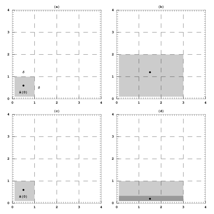
Figure 1: Schematic representation of the spreading of orbits in the neighborhood of a hyperbolic fixed point (origin) in the case of a non-conservative 2D dynamical system (a and b), or conservative system (c,d), see text for details. The numerical values in the coordinate axes are multiples of $\delta.$

If, now, we consider the case of a conservative system, in which $\lambda_{1}(T)$ and $\lambda_{2}(T)$ are reciprocal, the image of the set of orbits in the initial gray cell (figure 1c, in which we set $\lambda_{1}(T)=3$, $\lambda_{2}(T)=1/3$) is the dark gray area of the parallelogram shown in figure 1d. However, the vertical side of this parallelogram is now smaller than the accuracy limit $\delta$. Thus, if questions are made in order to identify in which cell the orbit is located, the search is restricted to a smaller number of cells $d=3$. In this case we have

$$S_{BG}=\ln d=\ln\lambda_{1}(T)\Rightarrow{S_{BG}\over T}={1\over T}\ln\lambda_{1}(T)={1\over T}\ln(\xi_{1}(T)/\xi_{1}(0))~{}~{}.$$ (2)

In the limit of large $T$ the quantities $(1/T)\ln\lambda_{k}(T)=(1/T)\ln(\xi_{k}(T)/\xi_{k}(0))$, $k=1,2$ yield the spectrum of Lyapunov characteristic exponents of the orbits (in the neighborhood of $O$). We see that in both cases, of Eq.(2.1) or Eq.(2), the rate of increase of the Boltzmann - Gibbs entropy $S_{BG}/T$ is given by the sum of positive Lyapunov characteristic exponents of the orbits, which according to Pesin’s theorem [22], is equal to the Kolmogorov-Sinai entropy of the orbital flow in the neighborhood of O. This means that the Kolmogorov-Sinai entropy is, in fact, a measure of the rate of change of the entropy rather than a measure of the entropy itself.

The following is a more precise treatment of the previous schematic picture. Consider a partitioning of the n-dimensional phase space ${\cal M}$ of a coservative system into a large number of volume elements of size $\delta^{n}$ for some small $\delta>0$. Let $\vec{x}(0)$ be the initial condition of an orbit located in a particular volume element $V_{0}=\xi_{01}\xi_{02}...\xi_{0n}$, where $\xi_{0k}$, $k=1,...,n$ are the linear dimensions of $V_{0}$ in a locally orthogonal set of coordinates in the neighborhood of $\vec{x}(0)$. Without loss of generality, we set all the initial values $\xi_{0k}$ equal, i.e., $\delta\equiv V_{0}^{1/n}=\xi_{0k}$, $\forall k$. All the orbits with initial conditions within $V_{0}$ are called ‘nearby’ to the orbit $\vec{x}(t)$ with initial condition $\vec{x}(0)$. Because of the volume preservation, the orbital flow defines a mapping $V_{0}\rightarrow V(t)$ of the volume $V_{0}$ to an equal volume $V(t)$ at the time $t$. We want to find an estimate of the covering of the cells of ${\cal M}$ by the volume $V(t)$ in terms of the variational equations of motion. To this end, let

$$\vec{\xi}(t)=D_{t}\vec{\xi}_{0}$$ (3)

be the solution of the variational equations for an initial deviation vector $\vec{\xi}_{0}$ acted upon by a linear evolution operator $D_{t}$ determined solely by the orbit $x(t)$. Let $\vec{\xi}_{k}^{\prime}(t)$ be the images of $\vec{\xi}_{0k}$, $k=1,2,...,n$ under the action of the operator $D_{t}$. The vectors $\{\vec{\xi}_{k}^{\prime}(t)\}$ form a complete basis of the tangent space to M at the point $\vec{x}(t)$ iff $\{\vec{\xi}_{0k}\}$ form a complete basis of the tangent space to ${\cal M}$ at the point $\vec{x}(0)$ and $rank(D_{t})=n$. It is possible to obtain an orthogonal basis $\{\vec{\xi}_{k}(t)\}$ starting from $\{\vec{\xi}_{k}^{\prime}(t)\}$ via the Gramm-Shmidt procedure [23]. The new basis is obtained by the recursive relation:

$$\vec{\xi}_{1}(t) = \vec{\xi}_{1}^{\prime}(t)$$

$$\vec{\xi}_{k}(t) = \vec{\xi}_{k}^{\prime}(t)-\sum_{\nu=1}^{k-1}\big{(}\vec{\xi}_{k}^{\prime}(t)\cdot\vec{\xi}_{\nu}(t)\big{)}{\vec{\xi}_{\nu}(t)\over\xi_{\nu}(t)^{2}}~{}~{}.$$ (4)

The volume $V(t)$ is given by $V(t)=\xi_{1}(t)\xi_{2}(t)...\xi_{n}(t)$. We reorder this basis by decreasing length of the vectors $\vec{\xi}_{k}(t)$. Let $V_{c}(t)$ be a coarse-grained volume equal to the total volume of all the cells visited by the orbits in $V(t)$. $V_{c}(t)$ is determined by only those vectors with lengths greater or equal to $\delta$, that is

$$V_{c}(t)=\xi_{1}(t)\xi_{2}(t)...\xi_{m}(t)\delta^{n-m}$$ (5)

where $m$ is defined by the condition $m=\sup\{m^{\prime}:\xi_{k}(t)\geq\delta\mbox{ for all }k=1,\ldots,m^{\prime}\}$. It follows that $m=n$ when $t=0$ and $V_{c}(0)=V(0)=\delta^{n}$.

The Boltzmann - Gibbs entropy is defined by

$$S_{BG}(t)\equiv\ln{W(t)}=\ln{\frac{V_{c}(t)}{V_{c}(0)}}$$ (6)

where

$$W(t)={\xi_{1}(t)\xi_{2}(t)...\xi_{m}(t)\over\delta^{m}}$$ (7)

yields the number of cells (or ‘micro-states’) occupied by $V_{c}(t)$.

The rate of growth of the entropy (6) for a set of nearby orbits is related to the spectrum of the Lyapunov characteristic exponents of the reference orbit $\vec{x}(t)$. The Lyapunov characteristic exponents are given by

$$\lambda_{k}\equiv\lim_{t\rightarrow\infty}{1\over t}\ln{\xi_{k}(t)\over\xi_{k}(0)}=\lim_{t\rightarrow\infty}{1\over t}\ln{\xi_{k}(t)\over\delta}$$ (8)

for $k=1,\ldots,n$, provided that the limits exist. Let $\lambda_{1},\lambda_{2},...\lambda_{m}$, $0\leq m\leq n/2$ be the set of positive exponents of the spectrum (8). According to Pesin’s (1978) theorem, their sum is equal to the Kolmogorov-Sinai entropy $S_{KS}$ of the flow of orbits ‘nearby’ to $x(t)$ [24, 25], i.e.

$$S_{KS}=\lambda_{1}+\lambda_{2}+...+\lambda_{m}~{}~{}~{}.$$ (9)

The average rate of increase of the Boltzmann-Gibbs entropy up to the time $t$ is given by $S_{BG}(t)/t$. In view of Eq.(7), the limit of this rate, for $t\rightarrow\infty$ is

$$\lim_{t\rightarrow\infty}\frac{S_{BG}}{t}=\lim_{t\rightarrow\infty}\frac{1}{t}\ln{W}=\sum_{k=1}^{m}\lambda_{k}=S_{KS}$$ (10)

Thus, in the limit $t\rightarrow\infty$ the Kolomogorov-Sinai entropy is equal to the asymptotic value of the mean growth rate of the Boltzmann-Gibbs entropy. Precise numerical examples of this relation were given in the case of low dimensional mappings [26, 7]. However, the orbits may exhibit transient or ‘metastable’ states for long time intervals before reaching the limit (10). Such states are characterized by a constant growth rate of the Tsallis q-entropy, to which we now turn our attention.

2.2 Tsallis entropy and the Average Power Law Exponent

The time evolution of the q-entropy [1] for an ensemble of orbits with initial conditions within the volume $V_{0}$ is given by

$$S_{q}(t)=\frac{W(t)^{1-q}-1}{1-q}~{}~{}.$$ (11)

In this equation $q$ is a constant parameter, known as the ’entropic index’ $q$. Dividing $S_{q}$ by $t/t_{1}$, where $t_{1}$ is a transient initial time of evolution of the orbits, and substituting $W$ from (7), yields the mean rate of evolution of $S_{q}$

$$\frac{S_{q}}{t/t_{1}}=\frac{1}{(t/t_{1})(1-q)}[(\frac{\xi_{1}\xi_{2}...\xi_{m}}{\delta^{m}})^{1-q}-1]~{}~{}.$$ (12)

For every $\xi_{k}$, $k=1,2,...m$, we define an Average Power Law Exponent (APLE) $p_{k}$ according to

$$\xi_{k}(t)=\xi_{k}(t_{1})(\frac{t}{t_{1}})^{p_{k}},~{}~{}~{}~{}~{}k=1,2,...m~{}~{}.$$ (13)

All the $p_{k}$ are, in general, functions of the time $t$, and the value of $p_{k}(t)$ yields the average logarithmic slope (or power-law exponent) of the evolution of $\xi(t)$ in the time interval from the time $t_{1}$ up to the time $t$. Furthermore, in conservative systems we have $p_{1}+p_{2}+...+p_{m}\geq 0$, since, by the preservation of volumes, the components $\xi_{k}(t)$ cannot be all decreasing functions of the time.

In view of the definition of the APLEs (13), equation (12)) takes the form

$${S_{q}\over t/t_{1}}={1\over(t/t_{1})(1-q)}\big{(}\big{(}{t\over t_{1}}\big{)}^{(p_{1}+p_{2}+...p_{m})(1-q)}-1\big{)}~{}~{}.$$ (14)

In the limit $t\rightarrow\infty$ the quantity $\frac{S_{q}}{t/t_{1}}$ tends to a non-zero finite value only if a) the $p_{i}$s take constant limiting values, and b) the entropic index $q$ satisfies the relation $(p_{1}+p_{2}+...p_{m})(1-q)=1$. In all other cases, $\frac{S_{q}}{t/t_{1}}$ tends either to zero or to infinity. If the deviations $\xi_{k}(t)$ grow asymptotically as a power law, then condition (a) is satisfied and the mean rate of increase of the Tsallis entropy $\frac{S_{q}}{t/t_{1}}$ tends to the sum of the positive APLEs

$$\lim_{t\rightarrow\infty}\frac{S_{q}}{t/t_{1}}=p_{1}+p_{2}+...p_{m}$$ (15)

for the value of $q$ given by

$$q=1-\frac{1}{p_{1}+p_{2}+...p_{m}}~{}~{}.$$ (16)

In that case, if $p_{1}$ is by definition the maximum of all the APLEs, this exponent can be used as a lower bound of the limit of $\frac{S_{q}}{t/t_{1}}$, i.e.

$$\lim_{t\rightarrow\infty}\frac{S_{q}}{t/t_{1}}\geq p_{1}~{}~{}.$$ (17)

In practice we can use Eqs.(15), (16), or (17) for a long but finite time $t$ in order to estimate the average value of the q-exponent in the interval from $t_{1}$ and $t$, provided that this value is almost constant in this interval. Furthermore, the ratio of the length of the deviation vector $\xi^{2}(t)=\sum_{k=1}^{m}\xi_{k}^{2}(t)$ at $t$ with respect to the length of this vector at $t_{1}$ can be evaluated from the equation

$$\frac{\xi^{2}(t)}{\xi^{2}(t_{1})}=\sum_{k=1}^{m}\frac{\xi_{k}^{2}(t)}{\xi^{2}(t_{1})}=\sum_{k=1}^{m}\beta_{k}^{2}(\frac{t}{t_{1}})^{2p_{k}}$$ (18)

where equation (13) has been used and

$$\beta_{k}^{2}=\frac{\xi_{k}^{2}(t_{1})}{\xi^{2}(t_{1})}$$ (19)

with

$$\sum_{k=1}^{m\leq n}\beta_{k}^{2}\leq 1~{}~{}.$$ (20)

Equation (18) can also be written as

$$\frac{\xi^{2}(t)}{\xi^{2}(t_{1})}=(\frac{t}{t_{1}})^{2p_{1}}[\beta_{1}^{2}+\sum_{k=2}^{m}\beta_{k}^{2}(\frac{t}{t_{1}})^{-2(p_{1}-p_{k})}]$$ (21)

Since $p_{1}-p_{k}$ is positive for $2\leq k\leq m$, the sum inside the square brackets in the last expression tends asymptotically to zero for $t>>t_{1}$. Thus we can write

$$APLE=p={\ln{\frac{\xi^{2}(t)}{\xi^{2}(t_{1})}}\over 2\ln{\frac{t}{t_{1}}}}=p_{1}+\frac{\ln{[\beta_{1}^{2}+\sum_{k=2}^{m}\beta_{k}^{2}(\frac{t}{t_{1}})^{-2(p_{1}-p_{k})}]}}{2\ln{\frac{t}{t_{1}}}}$$ (22)

i.e in the limit of $t\rightarrow\infty$ APLE tends to $p_{1}$.

In two dimensional maps or in the Poincaré surface of section of 2D Hamiltonian systems we have $m=1$, i.e. there is only one positive exponent $p_{1}$ which is the limit of APLE p. In these cases the APLE p is also the limit of the mean rate of growth of Tsallis entropy $S_{q}$ with $q=1-1/p$ according to (16).

2.3 The time evolution of APLE for weakly chaotic orbits and the appearance of ‘metastable’ states

In the sequel we are interested in the behavior of the deviations $\vec{\xi}(t)$ for orbits in the border of a single resonance domain of a nonlinear Hamiltonian system of $n$ degrees of freedom. In the integrable approximation this border is separatrix-like. The Hamiltonian in resonant normal form (see e.g. [27]) reads:

$$H={J_{\psi}^{2}\over 2}-\omega_{0}^{2}\cos\psi+H_{0}^{\prime}(J_{2},\ldots,J_{n})$$ (23)

in action -angle variables $(J_{\psi},J_{2},\ldots,J_{n})$ and $(\psi,\phi_{2},\ldots\phi_{n})$. The resonant variables $(J_{\psi},\psi)$, $J_{\psi}\in{\cal R}$, $\psi\in(\pi,\pi]$, obey a pendulum dynamics. The point $(J_{\psi},\psi)=\pi$ defines a foliation of simply hyperbolic $n-1$ dimensional invariant tori of (23) labelled by the constant values of $J_{i}$, $i=2,\ldots n$. In particular, when $n=1$ there is only a 0-dimensional torus, i.e. an unstable equilibrium point, while if $n=2$ the tori are 1-dimensional, i.e., a family of unstable periodic orbits. The remaining phase space is foliated by n-dimensional tori. The deviations $\xi(t)$ on these tori grow in general linearly $\xi(t)\approx\xi_{0}+A~{}t$, where $A$ is a measure of the frequency differences between orbits on nearby tori. We may assume that the derivatives $|\partial\omega_{i}/\partial J_{j}|\equiv|\partial^{2}H_{0}^{\prime}/\partial J_{i}\partial J_{j}|$ are bounded from above for all $i,j=2,\ldots,n$. This, however cannot be true for the frequency associated with either librations or rotations in the plane $(J_{\psi},\psi)$, since the derivative of either the libration or rotation frequency with respect to the resonant action tends to infinity when the action tends to its limiting value on the separatrix, i.e.:

$$\lim_{J_{r}\rightarrow J_{r,separatrix}}\bigg{|}{\partial\omega_{r}(J_{r})\over\partial J_{r}}\bigg{|}=\infty$$ (24)

where, e.g., for librations

$$J_{r}(E)=2\int_{\psi_{min}(E)}^{\psi_{max}(E)}J_{\psi}(E,\psi)d\psi$$ (25)

is the libration action of an orbit labeled by the energy $E=J_{\psi}^{2}/2-\omega_{0}^{2}\cos\psi$ and $\psi_{min}(E),\psi_{max}(E)$ are the limiting values of $\psi$ in the domain in which the latter equation has solutions. Furthermore $\omega_{r}(J_{r})=\partial E/\partial J_{r}$, and $J_{r,separatrix}=J_{r}(E=\omega_{0}^{2})$. A similar expression is found in the case of rotations, but with different limits of the integral (25). Near the separatrix, the value of $A$ in the linear term of the growth of deviations is determined essentially by the value of the derivative $a=|\partial\omega_{r}(J_{r})/\partial J_{r}|$, which is finite, but large. Thus the growth is essentially determined by the growth of the projection of the deviation vector on the plane $(J_{r},\phi_{r})$, where $\phi_{r}$ is the angle conjugate to $J_{r}$ according to the previous definitions. The variational equations for $\vec{\xi}\equiv(\Delta J_{r},\Delta\phi_{r})$ read

$$\dot{\Delta J_{r}}=0,~{}~{}~{}\dot{\Delta\phi_{r}}={\partial\omega_{r}\over\partial J_{r}}\Delta J_{r}$$ (26)

yielding the solution $\Delta J_{r}(t)=C=$ const., $|\Delta\phi_{r}(t)|=|\Delta\phi_{r}(0)+C~{}a~{}t|$. If $C=0$ the deviations remain constant $\xi(t)=|\Delta\phi_{r}(0)|$, while if $C\neq 0$ they grow linearly in time. In numerical applications we usually select a random orientation $\kappa=\Delta\phi_{r}(0)/\Delta J_{r}(0)\equiv\Delta\phi_{r}(0)/C$ for $\vec{\xi}_{0}$, so that, in general $C=\xi_{0}(1+\kappa^{2})^{-1/2}$ is of order $C=O(\xi_{0})\neq 0$ and $\xi(t)\approx\xi_{0}(1+at)$. The time behavior of the APLE for a deviation growing as $\xi(t)\approx\xi_{0}(1+at)$ is shown in figure 2a, when $a<1$ (curve (1)), or $a>1$ (curve (2)). In fact, when $t$ is large and $C=O(\xi_{0})$ we have $\xi(t)\approx\xi_{0}~{}a~{}t$, thus

$$p\simeq{\ln(\xi(t)/\xi_{0})\over\ln t}={1\over\ln t}(\ln a+\ln t)~{}~{}.$$ (27)

If $a<1$ we have $\ln a<0$ and $p$ tends to the value $p=1$ from below. On the other hand, if $a>1$ we have $\ln a>0$ and $p$ tends to the value $p=1$ from above. Thus, far from the separatrix the time evolution of $p$ is like in curve (1) of figure 2a, while close to the separatrix it is like in curve (2) of the same figure. Numerical examples of this behavior are given in section 3 below. Finally, independently of the distance from the separatrix, if the initial vector $\vec{\xi}_{0}$ is almost tangent to an invariant curve, we have $C<<\xi_{0}$. In that case we have $\xi(t)\simeq\xi_{0}$ and $p\approx 0$ for $t<1/C$, while for $t>1/C$ $p$ increases approaching asymptotically the value 1 from below, independently of the value of $a$ (figure 2a, curve 3). Numerically, we find that this behavior can only happen when the angle between $\vec{\xi}_{0}$ and the tangent to the invariant curve is small (below two degrees, see section 3). Near this value there is a continuous transition in a narrow interval of values of $\phi$ from the curve (3) to the curve (2). Practically, when the initial orientation of $\vec{\xi}_{0}$ is selected randomly, in the great majority of cases we encounter for regular orbits only the cases (1) and (2) of figure 2a.

Figure 2: The time evolution of $p$ vs. $\log_{10}t$ for (a) regular orbits, and (b) weakly chaotic orbits, according to the simplified model of Eq.(2.3). In (a) we have (1) $\xi=\sqrt{\Delta J_{r}^{2}+\Delta\phi^{2}}$ and $\xi_{0}=1$, $a=0.5$, $\epsilon\rightarrow 0$, (2) $\xi_{0}=1$, $a=2$, $\epsilon\rightarrow 0$, and (3) $\xi=1+\sqrt{\Delta J_{r}^{2}+\Delta\phi^{2}}$ with $\xi_{0}=10^{-2}$, $a=2$, $\epsilon\rightarrow 0$. In (b) we have (1) $\xi$ as in (a) with $\xi_{0}=1$, $a=0.5$, $\epsilon=10^{-6}$, (the Lyapunov exponent and upper crossover time are $\lambda\approx 10^{-3},t_{2c}\approx 10^{3}$) (2) $\xi_{0}=1$, $a=3$, $\epsilon=10^{-6}$, ($\lambda\approx 10^{-3},t_{2c}\approx 10^{3}$) (3) $\xi_{0}=1$, $a=3$, $\epsilon=10^{-8}$. ($\lambda\approx 10^{-4},t_{2c}\approx 10^{4}$) (4) $\xi_{0}=1$, $a=5$, $\epsilon=10^{-8}$. ($\lambda\approx 10^{-4},t_{2c}\approx 10^{4}$)

We now examine the time evolution of the APLE in the case in which a Hamiltonian perturbation is introduced, namely

$$H = {J_{\psi}^{2}\over 2}-\omega_{0}^{2}\cos\psi+H_{0}^{\prime}(J_{2},\ldots,J_{n})+\epsilon H_{1}(J,\phi;\epsilon)$$ (28)

$$= H_{r}(J_{r})+H_{0}^{\prime}(J_{2},\ldots,J_{n})+\epsilon H_{1}(J,\phi;\epsilon)~{}~{}.$$

In Eq.(28) we assume that an optimal resonant Birkhoff normal form has already been constructed (e.g. [27]). This means that the action - angle variables in (28) are obtained through a near-identity transformation from the original action - angle variables of the unperturbed Hamiltonian. Furthermore, in the Nekhoroshev regime the size of the perturbation $\epsilon$ in Eq.(28) is exponentially small in the quantity $1/\omega_{0}^{2}$. Ignoring the small components of the deviation vector normal to the resonant plane $(J_{r},\phi_{r})$, the new variational equations of motion read:

$${d(\Delta J_{r})\over dt} \simeq -\epsilon\big{(}{\partial^{2}H_{1}\over\partial J_{r}\partial\phi_{r}}\Delta J_{r}+{\partial^{2}H_{1}\over\partial\phi_{r}^{2}}\Delta\phi_{r}\big{)}$$

$${d(\Delta\phi)\over dt} \simeq \epsilon\big{(}{\partial^{2}H_{1}\over\partial J_{r}\partial\phi_{r}}\Delta\phi_{r}+{\partial^{2}H_{1}\over\partial J_{r}^{2}}\Delta J_{r}\big{)}+{\partial^{2}H_{r}\over\partial^{2}J_{r}}\Delta J_{r}~{}~{}.$$ (29)

While a detailed exploration of the solutions of Eqs.(2.3) can only be made after $H_{0}$ and $H_{1}$ are known, we can explore the basic behavior of the solutions close to the separatrix limit by the following heuristic analysis. Close to the separatrix we have $|\partial^{2}H_{r}/\partial J_{r}^{2}|=|\partial\omega_{r}/\partial J_{r}|>>1$, while $\partial\omega_{r}/\partial J_{r}<0$. Assuming that all the partial derivatives of $H_{1}$ in (2.3) have O(1) average values over the basic periods of motion, we introduce the following simplified model yielding essentially the behavior of the resonant components of the deviation vector:

$${d(\Delta J_{r})\over dt} = -\epsilon(\Delta J_{r}+\Delta\phi_{r})$$

$${d(\Delta\phi_{r})\over dt} = \epsilon(\Delta J_{r}+\Delta\phi_{r})-a\Delta J_{r}$$ (30)

for $a>1$ and $\epsilon<<1$. For $\epsilon=0$, Eqs.(2.3) take the form of the equations (26) of the integrable case. If we choose initial conditions perpendicular to the invariant curves of $H_{r}$, i.e., $\Delta J_{r}(0)=C=\xi_{0}$, $\Delta\phi_{r}(0)=0$, the solution of (2.3) reads:

$$\Delta J_{r}(t) = \xi_{0}\bigg{(}\cosh((a\epsilon)^{1/2}t)-\big{(}{\epsilon\over a}\big{)}^{1/2}\sinh((a\epsilon)^{1/2}t)\bigg{)}$$

$$\Delta\phi_{r}(t) = \xi_{0}\bigg{(}\big{(}{\epsilon\over a}\big{)}^{1/2}-\big{(}{a\over\epsilon}\big{)}^{1/2}\bigg{)}\sinh((a\epsilon)^{1/2}t)~{}~{}.$$ (31)

The asymptotic analysis of (2.3) yields now the reason why we observe a ‘metastable’ behavior in the time evolution of deviations. If $\epsilon<<1$, then for times $t<(a\epsilon)^{-1/2}$ we can consider both $\epsilon$ and $(a\epsilon)^{1/2}t$ as small quantities. Then, the first of equations (2.3) yields an almost constant term $\Delta J_{r}\approx\xi_{0}+O(\epsilon t)$, while the second equation yields a linear behavior $|\Delta\phi_{r}|\approx\xi_{0}|\epsilon-a|t$. This is similar to the case of regular orbits. We thus have a behavior similar to the curve (2) of figure 2a. However, when $t>(a\epsilon)^{-1/2}$ the exponential behavior becomes dominant $\Delta J_{r}\sim\Delta\phi\sim\exp((a\epsilon)^{1/2}t)$, with Lyapunov exponent $\lambda=(a\epsilon)^{1/2}$. This behavior is exemplified in figure 2b, in which we plot $\xi(t)=\big{(}\Delta J_{r}^{2}(t)+\Delta\phi_{r}^{2}(t)\big{)}^{1/2}$, with $\Delta J_{r}(t),\Delta\phi_{r}(t)$ given by Eq.(2.3), for different values of $a$ and $\epsilon$. We see that the combination of the linear and exponential laws creates a ‘plateau’ of nearly constant value of $p$ between an initial time $t_{1c}\approx 10$ and a second time $t_{2c}$ which is essentialy given by $t_{2c}\approx\lambda^{-1}$. These times are called ‘crossover times‘. In the interval $t_{1c}\leq t\leq t_{2c}$ the deviation vector $\xi(t)$ grows almost as a power law $\xi(t)\propto t^{p}$ for a nearly constant value of $p>1$. We stress that the real time evolution $\xi(t)\propto at+\exp(\lambda t)$ is mathematically different from a power law, and only a numerical resemblance to a q-exponential is systematically obtained for specific time intervals. As shown in figure 2b, the duration of the ‘metastable’ behavior decreases when $\lambda$ increases, while the value at which $p$ is stabilized in the interval $t_{1c}<t<t_{2c}$ increases as $a$ increases. An analytical estimate of the plateau is obtained by noticing that the leading terms of Eq.(2.3) (for small and large times) yield the time evolution of $\xi(t)$ more precisely as $\xi(t)\approx 1+at/2+(a/2\lambda)\left(e^{\lambda t}-1\right)$. Taking $p\simeq\ln\xi/\ln t$ we readily find the profile of the function $p(t)$ in the neighborhood of a characteristic time $t_{0}=1/\lambda$, given by the following bounds for the first and second derivatives of $p$ (for $\lambda\ll 1$):

$${dp\over dt}\leq\lambda\bigg{(}{2+1/e\over|\ln\lambda|}+{\ln(\lambda+ae/2)\over(\ln\lambda)^{2}}\bigg{)}$$

$${d^{2}p\over dt^{2}}\simeq\lambda^{2}\left({1-2/e-1/e^{2}\over|\ln\lambda|}+{1+\ln(a/2)-2/e\over(\ln\lambda)^{2}}+\frac{2\ln(ae/2)}{|\ln\lambda|^{3}}\right)>0~{}~{}.$$

The second of the above equations implies that the function $p(t)$ is convex at the time $t_{0}=1/\lambda$, so that the variations of $p$ over intervals $\Delta t$ around $t_{0}$ are bounded by the $O(\lambda/|\ln\lambda|)$ estimate for the first derivative, namely:

$$|\Delta p|\leq\lambda\bigg{(}{2+1/e\over|\ln\lambda|}+{\ln(\lambda+ae/2)\over(ln\lambda)^{2}}\bigg{)}\Delta t~{}~{}.$$ (32)

For example, if $\lambda=10^{-6}$, a 1% variation of the value of the APLE $\Delta p=0.01$ can only occur in an interval $\Delta t\sim 0.01|\ln/\lambda|/\lambda$, or $\Delta t\sim 10^{5}$. This value marks the extend of the plateau, which is a considerable fraction of the time $t_{0}\sim 1/\lambda$. The value of $p$ in this plateau is estimated as:

$$p_{plateau}\simeq 1+{\ln(ae/2)\over\ln|\lambda|}$$ (33)

The estimate (33) is found to be in good agreement with the numerical values of $p$ given, e.g., in the examples below. Recalling that $a$ is essentially a measure of the derivative of the frequency $|\partial\omega_{r}/\partial J_{r}|$, we expect that, in a chaotic layer resembling a separatrix, but with some thickness, $p$ increases as we approach to the center of the layer, since $a$ increases abruptly, while $p$ is smaller near the edges of the layer. This is precisely what is found in numerical experiments, as analyzed in the following section. In particular, if one defines an average value $\overline{<p>}$ over the whole chaotic layer, this yields an average value of the entropic index $q=1-1/\overline{<p>}$ corresponding to the metastable behavior of the orbits in this chaotic layer.

3 Numerical applications of the APLE

3.1 Separatrix layer in the 2D Standard Map

In the sequel we consider examples of numerical calculations of the APLE $\equiv p$ in discrete conservative systems. The time $t$ in Eq.(22) obtains discrete values $t=1,2,...$. In order to avoid a singular value of $p$ when $t=1$, we set $t_{1}=2$ and we calculate $p$ for $t\geq t_{1}$, with $p=0$ when $t=t_{1}$.

We are particularly interested in the time evolution of $p$ for orbits near or within a domain of weak chaos. A basic example is provided by the 2D standard map [28]:

$$y_{n+1} = y_{n}+\frac{K}{2\pi}\sin{(2\pi x_{n})},$$

$$x_{n+1} = x_{n}+y_{n+1},$$ (34)

where $x_{n}$, $y_{n}$ are given modulo(1) in the intervals [0,1) and [-0.5,0.5) respectively. Figures 3a,d show the phase portrait of the map (3.1) for $K=10^{-1}$ (figure 3a) and $K=10^{-2}$ (figure 3d). The thin solid lines in these figures are the unstable asymptotic manifolds emanating from the unstable periodic orbit $P_{U}\equiv(0,0)$. The manifolds are calculated by taking many initial conditions in a small segment of length $10^{-8}$ along the unstable eigendirection given by the monodromy matrix at $P_{U}$. Both phase portraits show the basic structure of the standard map for small $K$, i.e., a thin separatrix layer of weak chaos that separates a librational from a rotational domain. When $K$ is small the latter domains are filled almost entirely by invariant curves.

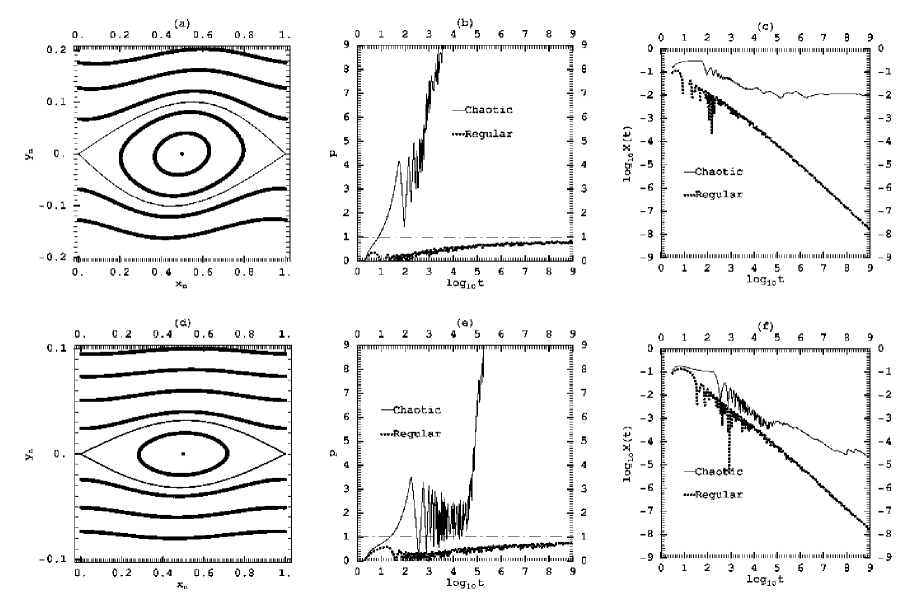
Figure 3: (a) phase portrait of the standard map for $K=10^{-1}$ (b) The time evolution of APLE for a regular orbit in the libration region of (a), and for a chaotic orbit in the thin separatrix layer, with initial conditions along the unstable manifold of the periodic orbit $(0,0)$. (c) the time evolution of the finite time Lyapunov number $\log_{10}\chi(t)$ for the same orbits. (d,e,f) same as in (a,b,c), but for $K=10^{-2}$.

Figures 3b,e show the typical time evolution of APLE for regular or chaotic orbits. The dotted curves give the time evolution of the APLE for a regular orbit inside the domain of librations (initial conditions: $(x_{0},y_{0})=(0.0,0.2)$, close to the stable periodic orbit at (0,0.5)), for $K=10^{-1}$ and $K=10^{-2}$. The initial deviation vector $\vec{\xi}(0)$ in both figures is chosen to be nearly perpendicular to the invariant curve passing through $(x_{0},y_{0})$. The temporal behavior of APLE in the dotted curves of figures.3b,e is typical of regular orbits, i.e., the APLE grows slowly tending asymptotically to $p=1$ from below (as in curve (1) of figure 2a). The oscillations of $p$ around its local mean value are due to oscillatory variations of the component of the deviation vector $\vec{\xi}(t)$ locally tangent to the invariant curve. In fact, if we approximate the invariant curve by an ellipse, it can be shown that the amplitude of the oscillations of $p$ is proportional to the axial ratio of the ellipse. Furthermore, a plot of the finite time Lyapunov number

$$\chi(t)={1\over t}\ln|{\xi(t)\over\xi(0)}|$$ (35)

for the same orbits (figures 3c,f, dotted lines) shows also the behavior expected for regular orbits, i.e., $\chi(t)$ falls asymptotically as $t^{-1}$ for large $t$.

Now, the thin solid curves in figure 3b,e show the behavior of APLE for chaotic orbits inside the separatrix layers of figures 3a,d. In this case we take the initial conditions on the unstable manifolds of $P_{U}$, a fact ensuring that all the consequents of the chaotic orbits are on the same manifolds. The initial deviation vector $\vec{\xi}(0)$ is chosen perpendicular to the unstable manifold. We can immediately notice the difference in the time behavior of APLE for these two orbits. In the case of the solid curve of figure 3e ($K=10^{-2}$), the APLE grows initially crossing the value $p=1$ at a short crossover time $t_{1c}=25$. However, after this crossing the APLE describes a number of oscillations around a mean value that remains systematically above unity, up to a second crossover time $t_{2c}=38.000$. We find $<p>=1.9$ in the time interval $t_{1c}\leq t\leq t_{2c}$. As shown in figure 3f, the value at which the finite time Lyapunov number $\chi_{(}t)$ stabilizes is $LCN\equiv\lambda=10^{-4.8}$. We thus see that the crossover time $t_{2c}$ is essentially given by $t_{2c}\approx\lambda^{-1}$. On the contrary, in the case of the solid curve of figure 3b ($K=10^{-1}$), the APLE grows from the start indefinitely, as expected for an exponential growth of deviation vectors, and there is no visible ‘metastable’ behavior in the time evolution of $p$. In that case the Lyapunov number (figure 3c) is rather large $\lambda=10^{-2}$, and the corresponding crossover time $t_{2c}\approx 10^{2}$ is of the same order as $t_{1c}$, i.e., extremely short to produce any visible effect.

As in the case of regular orbits, the oscillations of APLE around a local mean value in figures 3b,e are due to the oscillatory behavior of the component of the deviation vector $\vec{\xi}(t)$ which is tangent to a theoretical separatrix passing through the center of the separatrix chaotic layer. In this case we find that the first maximum value of $p$ in figures 3b,e occurs when the orbits pass close to the first homoclinic point of the unstable manifold emanating from $P_{U}$ and the stable manifold emanating from the image of $P_{U}$ modulo 1.

In order to check the dependence of the time evolution of the APLE on the initial orientation of the deviation vector $\vec{\xi}(0)$, corresponding to the value of the constant $C$ in the theoretical analysis of subsection (2.3), the following numerical test is performed: Starting from an arbitrary initial orientation of the deviation vector $\vec{\xi}(0)$, the orbit and the variational equations are integrated for a long time $t=\tau$. It is well known (see, for example [29]) that the deviation vector $\vec{\xi}(t)$ evolves so that it tends to become tangent to the invariant curve, in the case of a regular orbit, or parallel to the direction of a nearby unstable asymptotic curve (invariant manifold), in the case of a chaotic orbit. Let $(x_{\tau},y_{\tau})$ be the position of the orbit at $t=\tau$ and $(dx_{\tau},dy_{\tau})$ be the components of the deviation vector at this time. Taking $\tau$ long enough so as to ensure that the limit of tangency was reached down to the numerical precision level, we use $(x_{\tau},y_{\tau})$ and $(dx_{\tau},dy_{\tau})$ as the initial conditions of a second orbit and of its variational equations. We then compare the time evolution of the APLE for this deviation vector and for a second deviation vector associated to the same orbit, but with orientation forming an angle $\phi$ with $(dx_{\tau},dy_{\tau})$.

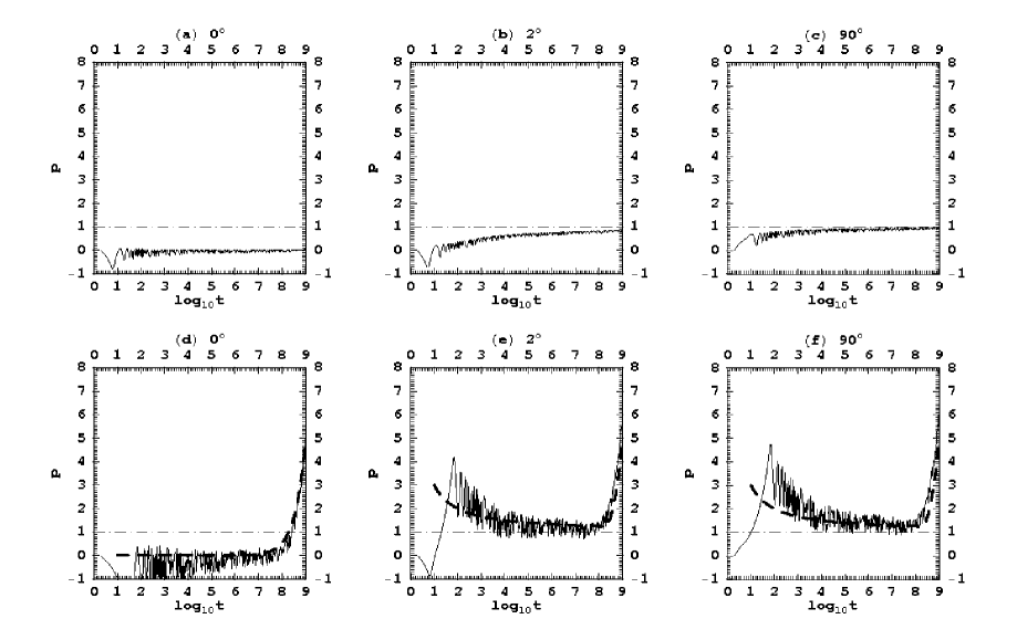
Figure 4: The time evolution of $p$ along a regular orbit with initial conditions $(x_{0},y_{0})=$ $(0.5000046134885427,$$0.08097827536667734)$, for $K=0.1$ and three different deviation vectors forming an initial angle (a) $0^{0}$, (b) $2^{0}$, (c) $90^{0}$ with the tangent to the invariant curve. The corresponding evolution for a chaotic orbit (initial condition $(0.5029208124108719,$$0.09994913824229859)$ is shown in (d-f), for $K=0.1$. The bold dashed line in (d) is the theoretical solution corresponding to an exponential law $\xi(t)/\xi_{0}=e^{\lambda t}$ with $\lambda=10^{-6.8}$, while in (e),(f) we superimpose to this a linear term $at$ with $a=2$.

Figure 4 shows examples of the dependence of APLE on the initial orientation using three different orientations, namely $\phi\simeq 0$, $\phi=2^{o}$ and $\phi=90^{o}$, in the case of a regular orbit with $K=0.1$ (first row in figure 4), and in the case of a chaotic orbit with $K=0.1$ (second row in figure 4). Clearly, the evolution of APLE is sensitive on $\phi$ only for small values of $\phi$. For example, in the case of the regular orbit, when $\phi\simeq 0$ (figure 4a) we have $\Delta J=C\simeq 0$ and the corresponding term in the solution of Eq.(26) is suppressed. Thus $\xi(t)$ simply makes oscillations around the mean value $<\xi(t)>=\xi(0)$, and the APLE remains close to a zero value even after $t=\tau=10^{9}$ iterations. On the other hand, when $\phi$ is equal to only $\phi=2^{o}$, the time evolution of APLE becomes already very similar to its typical behavior, as concluded by a comparison with the case $\phi=90^{o}$, corresponding to an initial deviation vector perpendicular to the invariant curve. The same phenomena apply to the case of weakly chaotic orbits as in the second row of figure 4. In that case, the asymptotic limit for all three values of the initial angle $\phi$ is an exponential growth of the corresponding deviation vectors, leading to a constant limit of the Lyapunov number $\lambda\simeq 10^{-6.8}$. When $\phi=0$ the ‘metastable’ behavior does not show up in the time evolution of the APLE. However, this behavior is clearly seen when $\phi\geq 2^{0}$, and it lasts up to the crossover time $t_{2c}\sim 10^{7}>10^{6.8}=1/\lambda$. In fact, plotting the theoretical solution (2.3) corresponding to a choice $\phi=90^{0}$ in this case shows a good agreement with the numerical results for both $\phi=2^{0}$ or $\phi=90^{0}$.

3.2 The APLE as a chaotic indicator measuring the entropic q-index. Comparison with FLI and MEGNO

In theory, the use of APLE as a ‘chaotic indicator’ distinguishing regular from chaotic orbits is straightforward. In the case of regular orbits the value of APLE tends to $p=1$ as $t\rightarrow\infty$, while in the case of chaotic orbits we have $p\rightarrow\infty$ as $t\rightarrow\infty$. In practice, however, one can only evaluate $p$ over a finite integration time $T$ and a numerical indicator of chaos is considered as efficient if this time is small. An example of efficient chaotic indicator that is widely used in the literature is the Fast Lyapunov Indicator (FLI) [15] in its revised form [30]. Let $\xi(t)$ be the length of the deviation vector of an orbit. The revised form of FLI reads:

$$FLI=\sup\{\ln\big{(}\xi(t)/\xi(0)\big{)},0\leq t\leq T\}~{}~{}.$$ (36)

In the case of regular orbits the deviations grow linearly, so that $\ln\big{(}\xi(t)/\xi(0)\big{)}\approx\ln t$. We can thus set a threshold value, say $FLI_{0}(T)=\ln 10+\ln T$, corresponding to a deviation vector larger by a factor ten from the one corresponding to the linear growth of deviations up to the time $t=T$. Then, if $FLI>FLI_{0}$ the orbit is called chaotic, otherwise it is called regular. In fact, if we are close to the border of a separatrix chaotic layer, we have $\xi(t)=\xi_{0}(1+a~{}t)$ for regular orbits, with $a>>1$ (subsection 2.3). Thus $\ln\big{(}\xi(t)/\xi(0)\big{)}\simeq\ln a+\ln t$. If we choose the threshold of $FLI_{0}$ as above, then, if $a>10$, a regular orbit can be erroneously characterized as chaotic. Thus, an improved formula for the threshold value is

$$FLI_{0}(T)=\ln 10+\ln a+\ln T$$

where the value of $a$ can be estimated by the value of $\xi(t_{1c})$ for a time $1<<t_{1c}<<T$, since, if $a>>1$, we have $\xi(t_{1c})\simeq\xi_{0}at_{1c}$. Then, the orbit is considered as chaotic if $FLI>FLI_{0}$ at the time $T$.

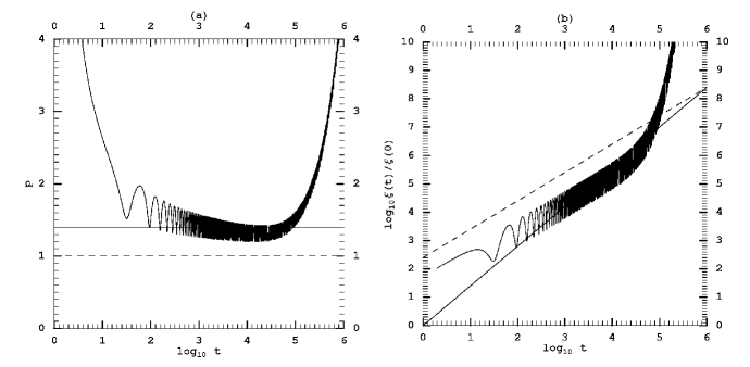
Figure 5: (a) A theoretical example of evolution of the APLE when an oscillatory term is added to the solution (2.3), namely $\xi=\sqrt{\Delta J_{r}^{2}+\Delta\phi^{2}}(1+\cos{0.1t})$ with $\Delta J_{r}$, $\Delta\phi_{r}$ given by Eq.(2.3) and $\xi_{0}=1$, $a=30$, $\epsilon=10^{-10}$. (b) The evolution $\log_{10}(\frac{\xi(t)}{\xi(0)})$ vs. $\log_{10}t$ for the same example. The dashed line corresponds to a linear law $\ln\xi(t)=\ln a+\ln t+\ln 10$, while the continuous line indicates a power-law $\xi(t)\propto t^{p}$ with ($p=1.4$, i.e., as given by the approximate plateau of (a).

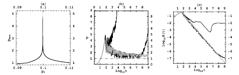
Figure 6: (a) The maximum value $p_{max}$ in a time interval $2<t\leq 10^{3}$ as a function of the initial condition $y_{0}$ of the orbits in a segment along the line $x_{0}=0.5$ crossing the separatrix domain of figure 3a. The peak value is for the orbit with initial conditions $(x_{0},y_{0})=(0.5,0.0998071243)$, and initial deviation vector $\vec{\xi_{0}}=(\frac{1}{\sqrt{2}},\frac{1}{\sqrt{2}})$. The evolution of the APLE and of $\log_{10}\chi(t)$ for the same orbit are shown as solid black curves in (b) and (c) respectively. The dotted black and the gray curves in the same plots correspond to orbits with initial conditions $(0.5,0.099807124)$ and $(0.5,0.09980712)$ respectively.

Suppose now that the orbit is weakly chaotic, so that a ‘metastable’ behavior exists for which $\xi(t)\sim\xi(t_{1c})(t/t_{1c})^{p}$, with $p>1$ (figure 5a, in which a plateau is formed at about $p=1.4$, from $t_{1c}=10^{3}$ to $t_{2c}=10^{5}$). As shown in figure 5b, the value of $\ln\big{(}\xi(t)/\xi(t_{1c})\big{)}$ crosses the line of $FLI_{0}(t)$ (solid straight line) at about the same time ($T=10^{5}$) when the slope of the quantity $\ln\big{(}\xi(t)/\xi(0)\big{)}$ vs. $\ln t$ crosses the value $p=1.4$ upwards, i.e. $t_{2c}\approx T$. This means that the APLE yields the characterization of the orbit as chaotic at the time $t_{2c}$ which is of the same order as the minimum time $T$ needed by the FLI. In fact, after $t>T$ the exponential growth of deviations becomes dominant and the slope of $\ln\big{(}\xi(t)/\xi(0)\big{)}$ vs. $\ln t$ tends very quickly to infinity.

In practice, we found that the location of thin chaotic layers in resonances can be determined using APLE in a way analogous to the Eq. (36), namely:

$$p_{max}=\sup\big{\{}p={\ln(\xi(t)/\xi(t_{1}))\over\ln(t/t_{1})},t_{1}<t\leq T\big{\}}~{}~{}.$$ (37)

In order to probe numerically the sensitivity of $p_{max}$ to thin chaotic layers, figure 6a shows the variation of the value of $p_{max}$, for $2<t\leq T=10^{3}$, along a segment of the line of initial conditions $x_{0}=0.5$ passing through the separatrix chaotic layer of figure 3a. As the center of the resonance is approached, the value of $p_{max}$ increases abruptly, the peak value marking clearly the center of the chaotic layer. The peak value of $p$ corresponds to an orbit with initial conditions $(x_{0},y_{0})\equiv$ $(0.5,0.0998071243)$ (the initial deviation vector is taken as $\vec{\xi}_{0}=(\frac{1}{\sqrt{2}},\frac{1}{\sqrt{2}})$). Since the chaotic layer is very thin, the behavior of APLE in a thin domain including this orbit is very sensitive on the choice of initial conditions. Thus, the central orbit has Lyapunov number $LCN\simeq 10^{-2}$ (figure 6c), and it shows only a small plateau in the values of $p$ at $p\simeq 3.5$, for about 900 periods, i.e., from $t=10^{2}$ to $t=10^{3}$ (figure 6b). However, if we only change the initial value $y_{0}$ by cutting the last digit, $(x_{0},y_{0})\equiv$ $(0.5,0.099807124)$, the new orbit has a much smaller Lyapunov number ($LCN\simeq 10^{-7}$, and the APLE forms a conspicuous plateau at $p\simeq 1.5$ which lasts for $10^{7}$ periods. Finally, if we cut one more digit in $y_{0}$, $(x_{0},y_{0})\equiv$ $(0.5,0.09980712)$, the orbit shows no sign of chaos up to $t=10^{9}$, although the plateau formed in the values of APLE (gray curve in figure 6b) is definitely at values $p>1$, an indication that the orbit may finally be chaotic. We notice that these results depend also on the machine precision, and different runs with different machines or precision levels yield qualitatively the same picture as in figure 6, but for somewhat different choice of initial conditions.

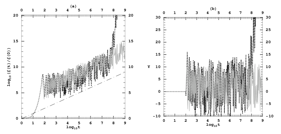
Figure 7: (a) The time evolution of $\log_{10}(\frac{\xi(t)}{\xi(0)})$, and (b) the time evolution of the MEGNO ($Y$) for the same orbits (gray and black dotted) as in figure 6b,c.

Figure 7a shows, for comparison, the identification of the same orbits as in figure 6 by the FLI. Clearly, the two methods have a similar sensitivity, i.e., $T\simeq t_{2c}=10^{8}$ for the dotted black curve of figure 7a. Figure 7b shows the behavior, for the same orbits, of yet a different chaotic indicator: the MEGNO [17]. The definition of MEGNO for continuous systems is:

$$Y(T)={2\over T}\int_{0}^{T}{\dot{\xi}(t)\over\xi(t)}tdt~{}~{}$$ (38)

whereas, in the case of mappings, $\dot{\xi}(t)$ is replaced by the finite difference of the deviations $\xi$ at successive time steps. If the deviations have an average power law behavior $\xi(t)\sim t^{p}$ in the interval $0\leq t\leq T$, Eq.(38) yields the value of MEGNO $Y=2p$. However, this is not so when the power-law is transient and approximate, i.e., it comes from a combination $\xi(t)\approx a~{}t+e^{\lambda t}$. In fact, for regular orbits we readily find $Y(T)=2(1-\ln(1+aT)/(aT)$, thus $Y(T)<2$ for $T>1/a$ even if $a>>1$, that is the MEGNO cannot yield a power-law exponent $p>1$. Furthermore, we find that the numerical behavior of the MEGNO shows variations which are about one order of magnitude larger than those of APLE in the whole interval of ‘metastable’ behavior of the orbits. This is exemplified in figure 7b, referring to the same orbits as in figure 6 or 7a. The fast oscillatory variation of the MEGNO, of amplitude $\Delta Y\approx 10$, shown in figure 7b results in that, while the maximum value of $Y$ is positive and above the threshold $Y=2$, the minimum value is negative. The mean value $<Y>$ in the transient interval of time is below $2$. On the other hand, not only the corresponding values of the APLE (figure 6b) are always positive, but they are clearly above the threshold $p=1$ during the whole interval $0\leq t\leq T$. Thus, the identification of the metastable behavior is much more clear by the APLE than by the MEGNO, and the APLE can be used to obtain a useful quantitative estimate of $<p>$, and thus of the entropic index $q=1-1/<p>$. This is shown in figure (8), which yields the average value of $<p>$ along an orbit in the time interval $0\leq t\leq T=10^{4}$, as a function of the orbit’s initial condition, for all the orbits in the same scanning of a thin chaotic layer as in figure 6. The general structure of this diagram is as in figure 6a. However, only a subset of these orbits have $<p>$ larger than unity. These orbits yield an average value of the values of $<p>$ equal to $\overline{<p>}=1.07$, corresponding to an entropic index $\bar{q}=0.065$.

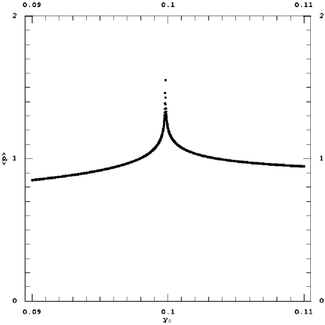
Figure 8: As in figure 6 but for the average value $<p>$ calculated over an interval of $10^{4}$ iterations per orbit.

3.3 Stickiness region

A case of particular interest, in which weak chaos emerges, is in the stickiness region at the border of an island of stability. The stickiness of the orbits is due to the existence of one or more cantori (see [31] for a review). The cantori arise from the destruction of KAM tori, which, according to Greene’s criterion [32] happens when the stable periodic orbits with rotation numbers forming sequences with limit equal to the rotation number of a torus become unstable [33, 34, 35, 36]. Since the dynamics at this limit is very close to hyperbolic, we expect that weakly chaotic orbits in the stickiness domain exhibit a transient metastable behavior for times of the order of the stickiness time.

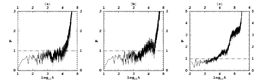
Figure 9: The time evolution of the APLE for some orbits belonging to the sticky region of an island of stability in the standard map for $K=5$ (see [37]). The initial conditions of the orbits are (a) $(x_{0},y_{0})=$ $(0.64337,0.36)$, (b) $(x_{0},y_{0})=$ $(0.6433684,0.36)$ and (c) $(x_{0},y_{0})=$ $(0.643363,0.36)$.

In order to study this phenomenon, we take initial conditions at the border of an island of stability as in [37], namely we consider initial conditions in a line segment with $y_{0}=0.36$ and $0.64324\leq x_{0}\leq 0.6434$ (as in figure 7 of [37]). The stickiness time is particularly high (it can be larger than $10^{6}$ periods) when $x_{0}>0.64336$. By integrating many chaotic orbits in this domain, we found three kinds of different behavior in the time evolution of the APLE, shown in figures (9)a,b,c respectively: (a) An orbit may form no ‘plateau’ beyond $p=1$ until the orbit escapes in the large chaotic sea outside the stickiness zone. (b) An orbit may form one plateau lasting for times of the order of its stickiness time, e.g. the orbit of figure 9b has a clear metastable behavior, with $p\simeq 1.3$ for $7000\leq t\leq 25000$, while the orbit escapes after about $10^{5}$ periods. (c) An orbit forms more than one ‘plateaus’ before escaping (the orbit of figure 9c forms two large plateaus at $p\simeq 1.5$ and $p\simeq 3$, lasting for about $10^{4}$ and $10^{5}$ periods respectively, while the stickiness time is about $5\times 10^{5}$ periods). The kind of behavior encountered by these orbits is very sensitive to the choice of initial conditions, a fact consistent with the fractal structure of the phase space near cantori.

3.4 The Arnold Web of a 4D Map

Chaotic indicators are widely used in order to visualize the Arnold web of resonances in multidimensional conservative systems. In the following numerical examples we consider the 4D symplectic mapping proposed in [20]

$$x_{j+1} = x_{j}-\epsilon\frac{\sin{(x_{j}+y_{j})}}{(\cos{(x_{j}+y_{j})}+cos{(z_{j}+t_{j})}+4)^{2}}$$

$$y_{j+1} = y_{j}+x_{j}~{}~{}~{}~{}~{}~{}~{}~{}~{}~{}~{}~{}~{}~{}~{}~{}~{}~{}~{}~{}~{}~{}~{}~{}~{}~{}~{}~{}~{}~{}~{}~{}~{}~{}~{}~{}~{}~{}~{}~{}~{}~{}~{}~{}~{}~{}~{}~{}~{}~{}~{}~{}~{}(mod2\pi)$$

$$z_{j+1} = z_{j}-\epsilon\frac{\sin{(z_{j}+t_{j})}}{(\cos{(x_{j}+y_{j})}+cos{(z_{j}+t_{j})}+4)^{2}}$$ (39)

$$t_{j+1} = t_{j}+z_{j}~{}~{}~{}~{}~{}~{}~{}~{}~{}~{}~{}~{}~{}~{}~{}~{}~{}~{}~{}~{}~{}~{}~{}~{}~{}~{}~{}~{}~{}~{}~{}~{}~{}~{}~{}~{}~{}~{}~{}~{}~{}~{}~{}~{}~{}~{}~{}~{}~{}~{}~{}~{}~{}(mod2\pi)$$

in order to study the behavior of APLE at the chaotic border of a single resonance domain. In this mapping, $(x_{j},z_{j})$ are action variables and $(y_{j},t_{j})$ are their conjugate angles. When $\epsilon=0$ we have constant values of the actions $x_{j+1}=x_{j}=x$, $z_{j+1}=z_{j}=z$, while the values $x,z$ yield also the frequencies, i.e., the per step changes of the angles. The lines $m_{1}x+m_{2}z$, with $m_{1},m_{2}$ integer, yield the Arnold web of resonances in the action plane. The chaotic motions in this mapping along the borders of resonances, when $\epsilon\neq 0$, were studied in detail in [39, 20]. Of particular interest are the chaotic motions when $\epsilon$ is smaller than a threshold value $\epsilon<\epsilon_{0}$ marking the onset of validity of the Nekhoroshev regime [38] (see [39]). In that case the chaotic motions can be identified to the phenomenon of ‘Arnold diffusion’ [40] (see [41] for a review).

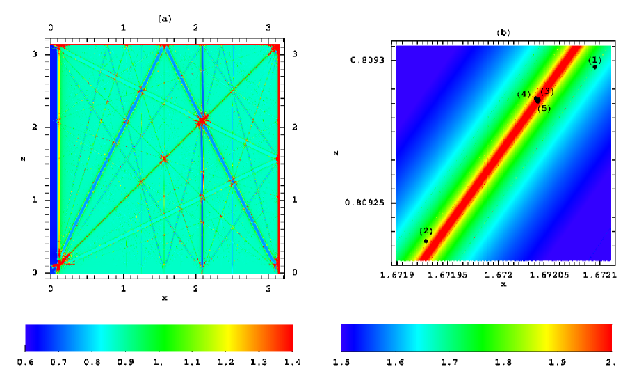
Figure 10: (a) A plot of the geography of the resonances in the action space of the 4D map (3.4) when $\epsilon=0.05$, by means of the index $p_{max}$ calculated over $T=10^{4}$ iterations per orbit. The initial conditions are in a $500$ uniform grid and the initial deviation vector for each orbit is $\vec{\xi}=(\frac{1}{\sqrt{2}},0,0,\frac{1}{\sqrt{2}})$. Each point is colored according to the value of $p_{max}$ in the range $0.6\leq p_{max}\leq 1.4$. (b) A zoom of (a) around the resonance $\frac{x_{j}}{z_{j}}=2$, produced from a set of $500\times 500$ initial conditions and the same vector $\vec{\xi}$ as in (a). The color scale for $p_{max}$ is in the range $1.5\leq p_{max}\leq 2$. The black points correspond to three initial conditions of orbits, namely $(x_{0},y_{0},z_{0},t_{0})=$ $(1.67209489949749,0,$ $0.809297781072027,0)$ (point (1)), $(1.67192854271357,0,$ $0.809236608877722,0)$ (point (2)), $(1.67203944723618,0,$ $0.809286279229481,0)$ (point (3)), $(1.67203675,0,$ $0.809286625,0)$ (point (4)), $(1.6720387,0,$ $0.80928565,0)$ (point (5)).

Numerical plots of the Arnold web on the action space can be obtained by plotting on a color or gray scale the value of a chaotic indicator as a function of the initial conditions of the orbits on the action space. Plots of this type, for different multidimensional Hamiltonian systems or mappings, were given, using different indicators [42, 43, 30, 20, 18, 44]. Here we use the APLE index $p_{max}$, for $T=10^{4}$ periods, in order to produce a plot of the Arnold web for the mapping (3.4), $\epsilon=0.05$. We set the initial values of the angles $y_{0}=t_{0}=0$ and use a $500\times 500$ grid of initial conditions on the action plane $(x_{0},z_{0})$. For all these orbits the initial deviation vector is $(dx_{0},dy_{0},dz_{0},dt_{0})=(\frac{1}{\sqrt{2}},0,0,\frac{1}{\sqrt{2}})$. The results are shown in figure 10a. The color scale corresponds to values of $p_{max}$ in the range $0.6\leq p_{max}\leq 1.4$, while, if the calculated value of $p_{max}$ for an orbit is outside the above interval, the associated color in the plot is replaced by that corresponding to the lower limit 0.6 or the upper limit 1.4.

The web of resonances is clearly visible in the plot of figure 10a, which is similar to plots of the same system produced in [20] using a different indicator, namely the FLI. Now, these authors studied in detail the diffusion in the action space of chaotic orbits starting at the chaotic border of a single resonance domain. When $\epsilon$ is sufficiently small, the system is in the ‘Nekhoroshev regime’ in which the diffusion coefficient is found to be exponentially small in the inverse of the perturbation, i.e., $D\propto\exp\big{(}-(\epsilon_{0}/\epsilon)^{b}\big{)}$ for some positive exponent $b$ (estimated as $b=0.28$ by the same authors). Since the diffusing orbits are in general very weakly chaotic, we expect that some of them exhibit the metastable behavior associated with a constant rate of production of the Tsallis q-entropy. We find this to be the case for some of the orbits explored in [20]. If a zoom of figure 10a is made in the neighborhood of a chaotic border of the resonance $x-2z=0$ (figure 10b), the orbits studied in [20] (their figure 5) correspond to the initial conditions
$(x_{0},y_{0})=(1.67209489949749,0,0.809297781072027,0)$ (point (1)) or
$(1.67192854271357,0,0.809236608877722,0)$ (point (2)) and
$(1.67203944723618,0,0.809286279229481,0)$ (point (3)). The point (3) is near a line passing from the center of the chaotic zone of figure 10b, while the two other points are near the edge of the same zone. Figure 11a then shows the time evolution of the APLE, $p$ vs. $\log_{10}t$ for these orbits. Clearly, in the case of the point (1) in figure 10b, the resulting orbits shows no visible metastable behavior, while such a behavior is clearly exhibited by the two orbits with initial conditions on the edge of the chaotic border. In fact, the calculation of the Lyapunov exponents $\lambda$ for these orbits [20] shows that the exponent of the first orbit is of order $\lambda\sim 10^{-2}$, while it is two orders of magnitude smaller $\lambda\sim 10^{-4}$ for the orbits near the edge of the chaotic border. We conclude that even if a system is in the ‘Nekhoroshev regime’, not all the chaotic orbits manifest the metastable behavior associated with the constant rate of production of the q-entropy, but only the orbits with initial conditions close to the edge of chaotic borders separating resonance from non-resonance domains.

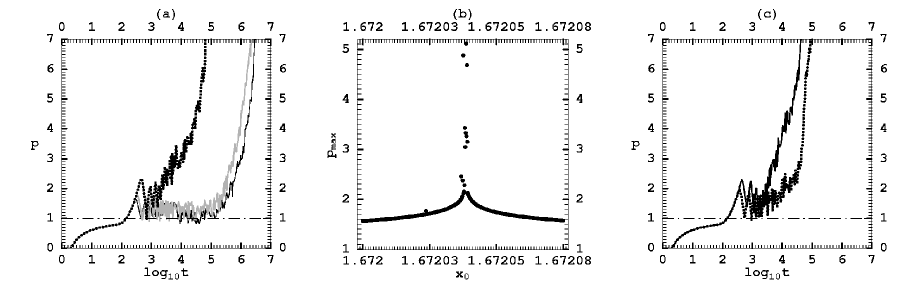
Figure 11: (a) The time evolution of the APLE for the three orbits with initial conditions as in figure 10b (thick dotted black curve for the point (1), gray curve for the point (2), and thin black for the point (3) point). (b) The value of $p_{max}$ after $T=10^{4}$ iterations as a function of the initial condition $x_{0}$ of a set of orbits in a segment crossing perpendicularly the resonance line of figure 10a. (c) Time evolution of $p$ for two orbits in the same line, with initial conditions as in figure 10b. The thick dotted line corresponds to the point (4) (orbit near the border of the resonance chaotic layer) and the thin continuous line to the point (5) (orbit near the center of the resonance chaotic layer).

Figure 12: As in 10a, but for the average value $<p>$ calculated over $10^{4}$ iterations per orbit.

In order to further substantiate this conclusion, figure 11b shows the value of $p_{max}$ for $T=10^{4}$ versus the value of the coordinate $x_{0}$ by a detailed scanning along a line passing through the chaotic border of figure 10b in the direction perpendicular to the direction of the resonance under study. We see that as the center of the chaotic border is approached the value of $p_{max}$ grows abruptly. This plot is similar to the plot of $p_{max}$ for the crossing of a thin separatrix chaotic layer in the 2D standard map (figure 6a), a fact expected since the dynamics near the chaotic border of a single resonance domain is qualitatively given by a separatrix-like map [28]. At any rate, figure 11b clearly shows that a relatively small value of the APLE (above unity), leading to a long lasting metastable behavior of the orbits, can be expected only near the edge of the chaotic border of the resonance. In fact, if we take two initial conditions along the scanning line of figure 11b (points (4) and (5) in figure 10b), the time interval of metastable behavior (figure 11c) is longer for the orbit (4), which is closer to the border of the chaotic layer than for the orbit (5) which is closer to the center of the layer. However, both orbits are relatively closer to the center than the orbits (1) and (2), and, consequently, they both have shorter metastable time intervals than the latter orbits (figure 11a).

Finally, figure 12 shows the average value $<p>$ over an interval $0\leq t\leq 10^{4}$ for all the orbits with initial conditions in the same interval as in figure 11b. These orbits have a value of $<p>$ always above unity, and the mean of all values in the interval is $\overline{<p>}=1.27$, yielding an entropic index $\bar{q}=0.21$.

4 Conclusions

We studied the connection between the production of Tsallis q-entropy and the behavior of the variational equations of motion for weakly chaotic orbits in conservative dynamical systems. Our main findings can be summarized as follows:

1) The solutions of the variational equations present long transient time intervals in which the length of the deviation vector increases almost as a power-law. This allows to define an almost constant average power-law exponent (APLE) during the whole transient interval.

2) This ‘metastable’ behavior can be justified theoretically by showing that it is caused by the growth of the deviation vectors inside separatrix-like thin chaotic layers, which is of the form $\xi(t)\approx at+e^{\lambda t}$, with $a>>1$ and $\lambda<<1$. The latter law appears almost as a power law $\xi(t)\approx t^{p}$ for time intervals up to $t_{2c}\approx\lambda^{-1}$.

3) The average value of the APLE in a thin chaotic layer can be used to determine an average value of the q-entropic index for which the Tsallis entropy exhibits a constant rate of increase.

4) The APLE can be used as an efficient numerical indicator distinguishing regular from weakly chaotic orbits. In that respect, it is equally powerful to other established indicators, as the FLI or the MEGNO. The advantage of the APLE is that it gives also the average value of the q-entropic index within a weak chaotic layer.

5) Numerical implementations of the APLE are given in low-dimensional symplectic mappings. The APLE is calculated in a thin chaotic layer and in the stickiness region of an island of stability in the 2D standard map. We then use it in order to visualize the Arnold web of resonances in a 4D map, and calculate the q-entropic index at the chaotic border of a single resonance domain of the same map.

Acknowledgements: G. Lukes-Gerakopoulos was supported in part by the Greek Foundation of State Scholarships (IKY) and by the Research Committee of the Academy of Athens. We thank Prof. G. Contopoulos for useful suggestions and a careful reading of the manuscript.

References

- [1] Tsallis C.: 1988, ‘Possible generalization of Boltzmann-Gibbs Statistics’ , J. of Stat. Phys., Vol. 52, pp. 479–487
- [2] Tsallis C., Rapisarda A., Latora V., Baldovin F. : 2002, ‘Nonextensivity: From Low-Dimensional Maps to Hamiltonian Systems’ , Lecture Notes in Physics , Vol. 602, pp. 140–164
- [3] Tsallis C., Plastino A. R., Zheng W.-M.: 1997, ‘Power-law sensitivity to initial conditions-new entopic representation’ , Chaos, Solitons and Fractals , Vol. 8, no. 6, pp. 885–891
- [4] Costa U. M. S., Lyra M. L., Tsallis C., Plastino A. : 1997, ‘Power-law sensitivity to initial conditions within logisticlike family of maps: Fractality and nonextensivity’ , Physical Review E , Vol. 56, no. 1, pp. 245–250
- [5] Lyra M. L., Tsallis C. : 1998, ‘Nonextensivity and multifractality in low-dimensional dissipative systems’ , Physical Review Letters , Vol. 80, no. 1, pp. 53–56
- [6] Baranger M., Latora V., Rapisarda A. : 2000 ‘Time evolution of thermodynamic entropy for conservative and dissipative chaotic maps’ , arXiv
- [7] Latora V., Baranger M., Rapisarda A., Tsallis C. : 2000, ‘The rate of entropy increase at the edge of chaos’ , Physics Letters A, Vol. 273, pp. 97–103
- [8] Grassberger P., Scheunert M.: 1981, ‘Some more universal scaling laws for critical mappings’ , Journal of Statistical Physics., Vol. 26 no. 4, pp. 697–717
- [9] Grassberger P.: 2005, ‘Temporal scaling at Feigenbaum points and nonextensive thermodynamics’ , Physical review letters., Vol. 95 no. 14, pp. 140601–1–140601–4
- [10] Robledo A.: 2006 ‘Incidence of nonextensive thermodynamics in temporal scaling at Feigenbaum points’ , Physica A, Vol. 370 no. 2, pp. 449–460
- [11] Baldovin F., Tsallis C., Schulze B.: 2003, ‘Nonstandard entropy production in the standard map’ , Physica A, Vol. 320, pp. 184–192
- [12] Baldovin F., Brigatti E., Tsallis C.: 2004, ‘Quasi-stationary states in low-dimensional Hamiltonian systems’ , Physics Letters A, Vol. 320, pp. 254–260
- [13] Añaños G. F. J. , Baldovin F., Tsallis C. : 2005 ‘Anomalous sensitivity to initial conditions and entropy production an standard maps: Nonextensive approach’ , European Physical Journal B, Vol. 46, pp. 409–417
- [14] Voglis N., Contopoulos G.: 1994, ‘Invariant spectra of orbits in dynamical systems ’ , Journal of Physics A: Mathematical and General , Vol. 27 no. 14, pp. 4899–4909
- [15] Froeschlé Cl., Gonczi R., Lega E.: 1997, ‘The fast Lyapunov indicator: a simple tool to detect weak chaos. Application to the structure of the main asteroidal belt.’ , Planet. Space Sci., Vol. 45 no. 7, pp. 881–886
- [16] Voglis N., Contopoulos G., Efthymiopoulos C.: 1998, ‘Method for distinguishing between ordered and chaotic orbits in four dimensional maps.’ , Physical Rev. E, Vol. 57 no. 1, pp. 372–377
- [17] Cincotta P.M., Simó C.: 2000 ‘Simple tools to study global dynamics in non-axisymmetric galactic potentials - I’ , Astronomy and Astrophysics Supplement , Vol. 147, pp. 205–228
- [18] Cincotta P.M., Giordano C.M., Simó C.: 2003 ‘Phase space structure of multidimensional systems by means of mean exponential growth factor of nearby orbits’ , Physica D, Vol. 182, pp. 151–178
- [19] Skokos, Ch.: 2001, ‘Alignment indices: a new, simple method for determining the ordered or chaotic nature of orbits.’, J. Phys. A: Math. Gen., Vol. 34, pp. 10029–10043
- [20] Froeschlé Cl., Guzzo M., Lega E.: 2005, ‘Local and global diffusion along resonant lines in discrete quasi-integrable dynamical systems’ , Planet. Space Sci., Vol. 45 no. 7, pp. 881–886
- [21] Schuster H. G. : 1995 , ‘Deterministic chaos’ , VCH , ed. 3
- [22] Pesin Ya. B.: 1977, ‘Characteristic Lyapunov exponents and smooth ergodic theory’ , Russian Math. Surveys, Vol. 52, no. 4, pp. 55–114
- [23] Benettin G., Galgani L., Giorgilli A., Strelcyn J.-M.: 1980, ‘Lyapunov characteristic exponents for smooth dynamical systems and for Hamiltonian systems - A method for computing all of them. I - Theory. II - Numerical application’ , Meccanica , Vol. 15, pp. 9–30
- [24] Kolmogorov A.N. : 1958, ‘A new metric invariant for transitive dynamical systems and automorphisms of Lebesgue Spaces’ , Dokl. Acad. Nauk SSSR , Vol. 119, pp. 861–864
- [25] Sinai Ya. G. : 1968, ‘Markov partitions and c-diffeomorphisms’ , Funct. Ana. Appl. , Vol. 2, no. 1, pp. 61–82
- [26] Latora V., Baranger M.: 1999, ‘Kolmogorov-Sinai Entropy Rate versus Physical Entropy’ , Physics Review Letters, Vol. 82, no. 3, pp. 520–523
- [27] Morbidelli A.: 2002 ‘Modern celestial mechanics. Aspects of solar system dynamics.’ , Taylor and Francis, London and New York
- [28] Chirikov B. V.: 1979, ‘Homogeneous model for resonant particle diffusion in an open magnetic confinement system’ , Sov. J. Plas. Phys., Vol. 5, pp. 492–497
- [29] Voglis N., Contopoulos G., Efthymiopoulos C.: 1999, ‘Detection of ordered and chaotic motion using the dynamical spectra.’ , Celest. Mech. and Dyn. Ast., Vol. 73 no. 1-4, pp. 372–377
- [30] Froeschlé Cl., Lega E.: 2000, ‘On the structure of symplectic mappings. The fast Lyapunov indicator: a very sensitive tool.’ , Celest. Mech. and Dyn. Ast., Vol. 78, pp. 167–195
- [31] Meiss J. D.: 1992, ‘Symplectic maps, variational principles, and transport.’ , Reviews of Modern Physics., Vol. 64 no. 3, pp. 795–848
- [32] Greene J. M.: 1979, ‘A method for determining a stochastic transition.’ , Journal of Mathematical Physics., Vol. 20 no. 6, pp. 1183–1201
- [33] Contopoulos G., Varvoglis H., Barbanis B.: 1987, ‘Large degree stochasticity in a galactic model.’ , Astronomy and Astrophysics., Vol. 172 no. 1-2, pp. 55–66
- [34] Contopoulos G., Harsoula M., Voglis N., Dvorak R.: 1999, ‘Destruction of islands of stability.’ , Journal of Physics A: Mathematical and General., Vol. 32 no. 128, pp. 5213–5232
- [35] Efthymiopoulos C., Contopoulos G., Voglis N., Dvorak R. : 1997, ‘Stickiness and cantori’ , J. Phys. A: Math. Gen., Vol. 30, pp. 8167–8186
- [36] Efthymiopoulos C., Contopoulos G., Voglis N.: 1999, ‘Cantori, Islands and Asymptotic Curves in the Stickiness Region’ , Celestial Mechanics and Dynamical Astronomy., Vol. 73 no. 1/4, pp. 221–230
- [37] Contopoulos G., Voglis N., Efthymiopoulos C., Froeschlé C., Gonczi R., Lega E., Dvorak R., Lohinger, E.: 1997, ‘Transition spectra of dynamical systems.’ , Celestial Mechanics and Dynamical Astronomy, Vol. 67 no. 4, pp. 293–317
- [38] Nekhoroshev N. N.: 1977, ‘An exponential estimate of the time of stability of nearly integrable Hamiltonian systems’ , Uspehi Mat. Nauk, Vol. 32, pp. 5–66
- [39] Guzzo M., Lega E.,Froeschlé Cl.: 2005, ‘First numerical evidence of global Arnold diffusion in discrete quasi-integrable systems’ , Discr. and Contin. Dynam. Systems, Vol. 5 no. 3, pp. 687–698
- [40] Arnold V. I.: 1964 ‘Instability of dynamical systems with several degrees of freedom.’ , Sov. Math. , Vol. 5, pp. 581–585
- [41] Cincotta P.M.: 2002 ‘Arnold diffusion: an overview through dynamical astronomy.’ , New Astronomy Reviews, Vol. 46 no. 1, pp. 13–39
- [42] Laskar J.: 1993, ‘Frequency analysis for multi-dimensional systems. Global dynamics and diffusion.’ , Physica D., Vol. 67 no 1-3, pp. 257–281
- [43] Kaneko K., Konishi T.: 1994 ‘Peeling the onion of order and chaos in a high-dimensional Hamiltonian system.’ , Physica D , Vol. 71, pp. 146–167
- [44] Giordano C. M., Cincotta P.M.: 2004 ‘Chaotic diffusion of orbits in systems with divided phase space.’ , Astronomy and Astrophysics, Vol. 423, pp. 745–753