The Fine Structure of Solar Prominences

Abstract

Solar prominences and filaments (prominences projected against the solar disk) exhibit a large variety of fine structures which are well observed down to the resolution limit of ground-based telescopes. We describe the morphological aspects of these fine structures which basically depend on the type of a prominence (quiescent or active-region). Then we review current theoretical scenarios which are aimed at explaining the nature of these structures. In particular we discuss in detail the relative roles of magnetic pressure and gas pressure (i.e., the value of the plasma-$\beta$), as well as the dynamical aspects of the fine structures. Special attention is paid to recent numerical simulations which include a complex magnetic topology, energy balance (heating and cooling processes), as well as the multidimensional radiative transfer. Finally, we also show how new ground-based and space observations can reveal various physical aspects of the fine structures including their prominence-corona transition regions in relation to the orientation of the magnetic field.

Astronomical Institute AS, Ondřejov, Czech Republic

1 Introduction

Solar prominences have been observed since the invention of the spectrohelioscope and as an example one can see well-known H$\alpha$ drawings by Secchi (1877) (one can be found in the textbook of Tandberg-Hanssen (1995)). Although these pioneering observations were rather simple, they already indicate that prominences consist of many complicated structures having seemingly chaotic behaviour. Prominence fine structures have then been frequently observed with better and better resolution, reaching today a hundred of km. However, although the fine structure was known, the prominences have been modeled for decades as a whole, using simplified one-dimensional (1D) slab models. Their magneto-hydrostatic (MHS) structure was first derived by Kippenhahn & Schlüter (1957) (hereafter referred to as KS-model) and their radiative properties were studied in a 1D-slab approximation by many authors. Such models reproduced rather well the spectral properties of prominences as observed with lower resolution. The aim of this review is to discuss various aspects of current investigations of prominence fine structures. This topic was thoroughly reviewed by Heinzel & Vial (1992), while Engvold (2004) summarized the latest observational results achieved with the highest resolution. Some aspects of prominence fine structures related to space research were briefly discussed by Vial (2006). For a more general description of the prominence physics the reader is referred to the monograph of Tandberg-Hanssen (1995).

2 Morphology of Prominence Fine Structures

Prominence fine-structure morphology manifests itself rather differently in case of the limb observations and in case of disk filaments. Moreover, one has to clearly distinguish between typical quiescent and active-region prominences or filaments. Generally speaking, a prominence seen on the limb has appeared before or will appear later as a filament on the disk. In case of quiescent prominences larger-scale structures remain fixed while the fine structure changes rather rapidly. However, it seems to be very difficult to identify the same structures as seen on the limb and on the disk – this makes a lot of confusion and we will discuss this later.

Our information about the fine structure morphology and dynamics comes from currently available high-resolution ground-based observations mostly made in the H$\alpha$ line. With the instruments like the new SST (Swedish 1-m Solar Telescope) or DOT (Dutch Open Telescope), one can see fine structures down to the resolution limit (0.15^′′ for SST or around 100 km). Homogeneous time series are now expected with a similar spatial resolution from the Solar Optical Telescope (SOT) onboard the Hinode satellite. A large variety of fine structures and their dynamics is also seen on TRACE movies, although the spatial resolution is lower, around 1^′′ (see e.g., TRACE filament movies on DVD provided by LMSAL). These images are usually taken with a 171 or 195 Å filter where the hot coronal structures appear simultaneously with cool ones – see Fig. 1. Cool prominences or filaments are dark against the bright background which is due to the absorption of the background coronal radiation emitted in these lines by the hydrogen and helium resonance continua (see cartoon in Rutten (1999)) and partially due to lack of emissivity of the TRACE lines within a volume occupied by cool prominence plasmas. At 171 or 195 Å, the He I and He II absorption dominates over the H I and it was shown theoretically that this opacity is quite comparable to that of the H$\alpha$ line (Anzer & Heinzel 2005).

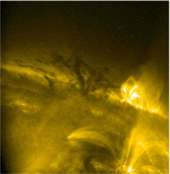
Figure 1.: TRACE image of a limb prominence taken in the 195 Å  line. Note the fine structures which appear very dynamic on the respective TRACE movies.

A large quiescent prominence observed at Big Bear Solar Observatory (see Fig. 2) exhibits many vertically oriented threads of the cool plasma which are a few hundred kilometers wide (from Low & Petrie (2005)). On a larger scale, one can identify a few vertical plasma sheets which, using a lower spatial resolution, would appear as more-or-less homogeneous slabs with the thickness typically smaller compared to the other two spatial dimensions. Such a kind of low-resolution images led modelers to use a vertical 1D slab approximation to a real prominence geometry which completely neglected the fine structure. In case of MHS models we already mentioned the classical KS solution. To handle the non-LTE radiative transfer, 1D slab models were extensively used starting from Poland & Anzer (1971), Yakovkin & Zel’dina (1975) and others. We will not detail these models here but rather discuss their recent generalizations to fine-structure modeling.

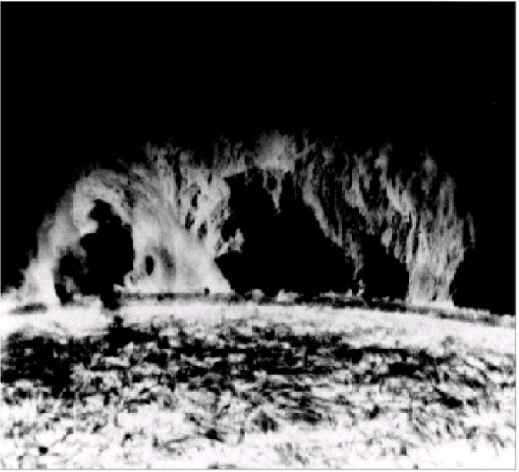
Figure 2.: Big Bear Solar Observatory (BBSO) image of a typical quiescent prominence. Quasi-vertical plasma threads are well visible (from Low & Petrie (2005)).

On the disk, the high-resolution H$\alpha$ images or movies show fine-structure fibrils of different lengths, the thinnest visible down to the resolution limit of SST or DOT. Very thin dark fibrils (we call them “fibrils” to distinguish them from vertical “threads” seen on the limb) visible along the spine of a quiescent filament are rather short and inclined to the filament axis due to the shear of the magnetic field lines (Fig. 3). On the other hand, much longer fibrils can be seen within the barbs or connecting various parts of the filament main body (Fig. 4). The fact that densely packed fibrils seen along the spine are rather short compared to a large-scale magnetic arcade in which the prominence/filament sits indicates that these fibrils are locations of cool plasma condensations in a presumably dipped magnetic field.

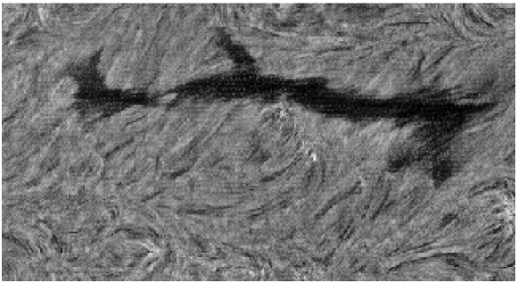
Figure 3.: Dutch Open Telescope (DOT) image of a disk filament. Many dark fibrils are seen along the filament spine and elsewhere (courtesy of R.J. Rutten).

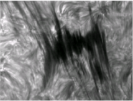
Figure 4.: Swedish 1-m Solar Telescope (SST) image of a disk filament. Here we can see long dark fibrils which resemble rather thin flux-tubes (courtesy of O. Engvold).

3 Dynamics of Prominence Fine Structures

While the large-scale quiescent prominence structure is rather stable, the fine structures described above exhibit a strongly dynamical behaviour. Their shape and brightness change on time scales of minutes which was already noticed by Engvold (1976) using the H$\alpha$ prominence observations made at the Dunn VTT at Sacramento Peak. Today one can study the fine-structure dynamics and prominence evolution on prominence/filament movies taken by TRACE in the 195 Å  line or on high-resolution H$\alpha$ images or movies. Within the disk filaments, individual fibrils move sideways with velocities up to 3 km  s^-1 which seems to be consistent with limb observations of Zirker & Koutchmy (1990, 1991). A qualitatively new observation was reported by Zirker et al. (1998) who identified a kind of streaming and counter-streaming in a filament in both spines and barbs, having flow velocities around $15\pm 10$ km s^-1. Dark H$\alpha$ knots were tracked for distances of 10⁴ to 10⁵ km at these speeds – see long arrows in Fig. 2 of Zirker et al. (1998).

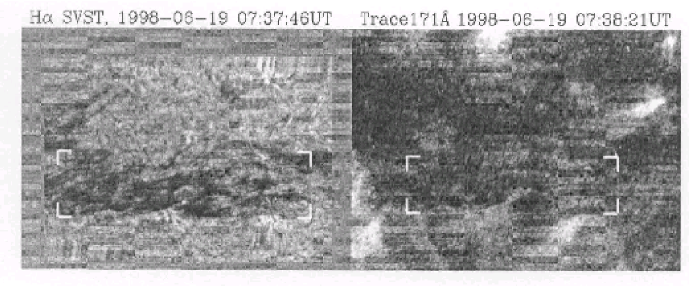
Figure 5.: H$\alpha$ and TRACE fine-structure fibrils. The spatial resolution of TRACE is lower, but same dark fibrils can be well identified on both images (from Schmieder et al. (2004)).

The same counter-streaming was further observed by Lin et al. (2003) using the high-resolution SST H$\alpha$ images and Dopplergrams. Both Zirker et al. (1998) and Lin et al. (2003) interpret these motions as plasma flows along the magnetic flux tubes which are not dipped. We have an evidence that these high-resolution H$\alpha$ images show fine structures which are well coaligned with dark features visible in the same filament on TRACE 195 Å  images – see Fig. 5 from Schmieder et al. (2004). These authors have studied the same filament as Lin et al. (2003).

4 Thermodynamic Properties from Spectral Diagnostics

Spectral diagnostics of prominence fine structures is a difficult task for several reasons. First, one has to distinguish between optically-thin and optically-thick fine structures. In the former case several fine-structure elements (FSE) are seen along the line of sight and their radiation output is thus integrated. On the other hand, in case of thick structures, we mostly see only one FSE, most probably located closer to the border of a prominence rather than in its central parts. The situation is actually more complex, because an optically-thick FSE is thick in the line core but becomes thin in the line wings, where we again see many FSE along the line of sight. This situation largely complicates the analysis of spectral data. Second reason is that, as already mentioned above, FSE are highly dynamical and thus any multi-wavelength observation has to be made simultaneously or at least quasi-simultaneously (this means within time shorter than the life-time of the FSE) in all wavelength bands of interest. Another complication arises from the lack of our detailed knowledge about the internal structure of FSE and their distributions within a prominence – even their elementary geometry is subject of a controversial debate (vertical threads, horizotal fibrils with flows, blobs etc.). For spectroscopic work, two basic models are usually considered: (i) Each FSE has its own prominence-corona transition region (PCTR), its 3D shape will then depend on the magnetic field threading the FSE because of principally different thermal conductivity along and across the field lines, (ii) FSE are more-or-less isothermal, but their temperature increases towards the prominence boundaries and this forms another kind of PCTR on a larger scale. A combination of (i) and (ii) is also possible. For further details and references see the review by Vial (1998) and his recent summary at the SOHO-17 workshop (Vial 2006). The scenario (i) was corroborated by various authors, while the second one (ii) was suggested e.g., by Poland & Tandberg-Hanssen (1983) who analyzed the spectral data from SMM/UVSP. Here it is worth mentioning that the scenario (ii) allows one to use a 1D slab model with a relevant PCTR on each side as a first approximation (see Anzer & Heinzel (1999)), while the effect of a fine-structure PCTR (case (i)) has to be modeled by considering a superposition of several FSE (each of them, however, can be again modeled by a simple 1D slab which describes, contrary to (ii), only one FSE) – see Vial et al. (1989), Heinzel (1989) or Fontenla et al. (1996). Finally, a principal difficulty in our understanding of the thermodynamical properties of prominence plasmas comes from the nature of radiation processes involved. The prominence spectral lines are mostly formed, namely in cooler parts, by the scattering of the incident radiation coming from the solar surface (photosphere, chromosphere, or even PCTR, depending on the spectral line under consideration). This leads to strong departures from LTE and thus the non-LTE theory of radiative transfer must be applied to prominences and filaments. This is known for a long time, here we can mention pioneering works by Poland & Anzer (1971), by an HAO group in the seventies (see Heasley & Milkey (1978) and references therein) or by Kiev groups (Yakovkin & Zel’dina (1975), Morozhenko (1984)). For a recent summary of modern non-LTE techniques see Heinzel & Anzer (2005). The use of these transfer methods for 1D slabs is almost routine today and several 1D non-LTE codes do exist: the IAS code (Gouttebroze & Labrosse 2000), the Ondřejov code (Heinzel 1995), PANDORA is now also being modified to prominence slabs (Heinzel & Avrett 2007). 2D slab models were considered first by Vial (1982) using the MAM code of Mihalas et al. (1978), then by Auer & Paletou (1994) and Paletou (1995) and finally by Heinzel & Anzer (2001). All these codes can be or have been used to model either the prominence or filament as a whole (note: for prominences one uses slabs standing vertically above the solar surface, while in case of filaments the slabs are horizontal, i.e., parallel to the solar surface) or individual FSE. However, in case of several FSE, the situation becomes much more complex because of their mutual radiative interaction. This was treated in simplified ways by Zharkova (1989) and by Heinzel (1989), but in most other cases the radiative interaction was neglected, all FSE were considered the be identical (as 1D slabs) and simply superimposed along the line of sight (Fontenla et al. (1996); Heinzel et al. (2001)). This interaction could, however, be tackled using todays high-performance parallel machines.

In the above summary we have tried to give the reader an idea how complex the spectral diagnostics of prominence fine structure is. However, we still completely neglected the dynamics or temporal variations of thermodynamic properties. The actual values of thermodynamic parameters like the kinetic temperature ($T$), gas pressure ($p$), plasma density ($\rho$), electron density ($n_{\rm e}$), but also the number of FSE along the line of sight or their geometrical dimensions, derived from prominence/filament spectra, have been summarized e.g., by Tandberg-Hanssen (1995), Vial (1998) or recently, using SOHO/SUMER data, by Patsourakos & Vial (2002). One approach is to study in detail the properties at a given prominence location, where we see – as discussed above – one or more FSE along the line of sight, or to perform a statistical analysis of the raster data to get the information about a global distribution of such parameters. Here we can mention the recent work by Wiehr et al. (2007) (see also López Ariste & Aulanier (2007) on p. 291 ff in this volume), where the line ratio technique (He D₃ over H$\beta$) was used. The results based on high-resolution filtrograms taken on VTT at Tenerife do indicate distinct situations: The case when for example the gas pressure would be almost constant over the prominence region (see also Stellmacher & Wiehr (2005)) is of a particular interest since it indicates an almost linear decrease of the magnetic field intensity with height and a statistical homogeneity of the spatial distribution of FSE.

4.1 Spectral diagnostics with SOHO

A few months before this Coimbra meeting solar physicists celebrated 10 years of successful observations with the Solar and Heliospheric Observatory (SOHO), which is a joint ESA/NASA mission (see proceedings from SOHO 17 Workshop held in Sicily, May 2006 – ESA SP-617). During this period, SOHO was frequently used to observe solar prominences and filaments in UV and EUV spectral bands. In particular SUMER and CDS spectrometers provided us with a wealth of unique data. The use of SUMER for prominence physics was reviewed by Patsourakos & Vial (2002), prominence spectroscopy with SUMER was also summarized by Heinzel et al. (2006). Concerning the prominence fine structure, Wiik et al. (1999) and Cirigliano et al. (2004) have studied the behaviour of lines formed in PCTR, while Heinzel et al. (2006) give a summary of their work on the hydrogen Lyman spectrum. The Lyman lines of hydrogen were also studied by Aznar Cuadrado et al. (2003). Finally, let us mention that Parenti et al. (2004) and Parenti et al. (2005) have produced an atlas of the prominence EUV spectrum observed by SOHO/SUMER.

5 Magnetic Field Determinations

Magnetic fields in solar prominences were measured since several decades, using first the Zeeman technique and later on the Hanle effect. This is summarized in the review by López Ariste & Aulanier (2007) on p. 291 ff in this volume. Older polarimetric observations made with the coronagraph led, in the case of quiescent prominences, to magnetic fields typically below 20 G. For latitudes larger than 35^∘ one obtains a mean value of $B$ equal to 8 G, while at lower latitudes the mean field is around 10 G (Bommier et al. 1994). Leroy et al. (1983) analyzed data for a large number of polar-crown filaments and found $B$ in the range 2 – 15 G, while Athay et al. (1983) arrived at values 6 – 27 G for a sample of 13 prominences (however, they didn’t distinguish between quiescent and eruptive prominences). Practically all these measurements have indicated the predominance of horizontal fields which naturally posses the question why the fine-structure threads appear quasi-vertical and not aligned along the field lines like the magnetic flux-tubes (Leroy 1989).

More recent measurements seem to indicate higher fields, reaching values of a few tens of Gauss (López Ariste & Aulanier (2007)). However, the respective observations concern only a rather restricted sample of prominences which may not always be of a quiescent type or are restricted to low parts of prominences (including their feets). Higher fields also follow from the analysis of the Stokes $V$ – signal which was not used in earlier studies. The actual intensity of the magnetic field is critical for our understanding of the prominence support and we will discuss this in the next Section.

6 Magnetic Models of Fine Structures

Since the fine-structure magnetic fields have not yet been detected (not because of lack of the spatial resolution, but due to still a low signal-to-noise ratio in polarimetric signals), most of our current knowledge or ideas come from data-driven modeling. Either one can use the detailed distribution of surface magnetic fields (like the SOHO/MDI maps) and perform coronal extrapolations of various degrees of sophistication (see review by López Ariste & Aulanier (2007) in this volume), or use indirect spectroscopic methods and modeling to infer the fine structure of the magnetic field (like that suggested in Heinzel et al. (2001) and recently used in Schmieder et al. (2007)). Here we are mainly interested in the topology of the field inside and in the surroundings of FSE (for a recent summary see also Anzer (2002)).

Two different magnetic configurations are considered in relation to prominence fine structures. The first one, also discussed by López Ariste & Aulanier (2007), is based on the assumption that the plasma-$\beta$ (ratio of gas to magnetic pressure) is always very low, of the order of 10^-2 or lower. In that case, the plasma itself has negligible effect on the topology of magnetic fields related to FSE. If, however, the plasma-$\beta$ is larger, of the order of 0.1 – 1.0 or even higher, the weight of the plasma will produce what we call “gravity-induced magnetic dips”. Let us discuss these two situations in more detail (see also Anzer (2002)).

6.1 Low-$\beta$ models

The topology of the prominence magnetic fields at low $\beta$ is discussed by López Ariste & Aulanier (2007) on p. 291 ff so that we give only a brief overview here. Today various authors try to model the prominence magnetic field by linear or non-linear force-free-field (“fff”) extrapolations of the measured photospheric field. Aulanier & Démoulin (1998) show that the prominence may consist of many rather shallow magnetic dips which can be filled by the cool material visible e.g., in the H$\alpha$ line. The presence of such dips was further demonstrated by Aulanier & Schmieder (2002) and by Aulanier & Démoulin (2003). In the latter paper the authors studied several prominences and found that the extrapolated field strength is rather low for typically quiescent prominence (less that 10 G), higher than 10 G for a plage filament and can reach 30-40 G for active-region prominences. This clearly shows how important the knowledge of the prominence type is: when we speak about the fine structure of quiescent prominences (as in this review), we cannot use measurements obtained for other types of structures. Some of the recent measurements which indicate rather strong fields seem to be related to more active structures. Moreover, these new measurements were not obtained using the coronagraphs and thus, because of scattered light higher above the limb, the measurements are more restricted to lower heights where the prominences appear brighter and where the polarization signal/noise ratio is sufficient (López Ariste – private communication). The usefulness of the filament modeling with linear fff was rather convincingly demonstrated by Aulanier et al. (2000) who performed a kind of “blind test”: magnetic dips obtained from numerical extrapolation were marked by black bars schematically indicating the location of the absorbing H$\alpha$ material – see Fig. 6. The shape of the filament and its various parts were then compared with the true shape as observed on the disk in H$\alpha$ and the agreement is quite reasonable. Non-linear fff models were considered e.g., by van Ballegooijen (2004).

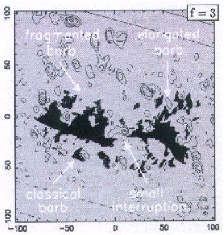
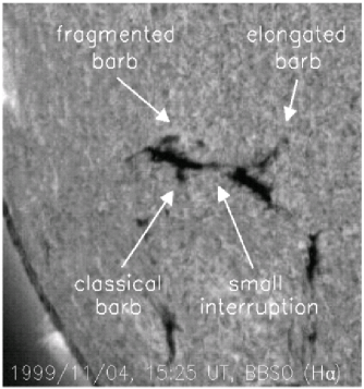
Figure 6.: Computed dark-fibril pattern from linear fff extrapolations (left) and the corresponding filament observed in the H$\alpha$ line (right). See the text where this “blind” test is described. From Aulanier et al. (2000).

For a given curvature of the magnetic dip, Aulanier & Schmieder (2002) assumed that the dip is filled by cool plasma up to one pressure scale-height $H=kT/g\mu$, where $\mu$ is the mean molecular mass (Fig. 7). For typical prominence conditions $H$ is of the order of 200 km. With the computed curvature of the fff dips one can draw the bars which indicate the presence of the absorbing material and have the length 2$l$ as indicated in Fig. 7. However, the real distribution of the opacity will depend on the actual dip configuration, mass loading in it and on various plasma parameters including the hydrogen excitation/ionization conditions. This was not so far considered in the context of fff models.

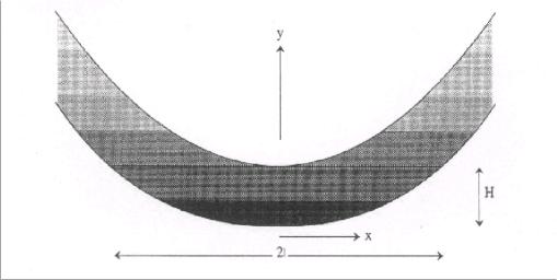
Figure 7.: A schematic model showing how the magnetic dip is filled by the plasma up to one pressure scale-height $H$. A corresponding horizontal extension of the mass loading is 2$l$. From Priest (1990).

6.2 Gravity-induced dip models

Spectroscopic determinations of the plasma density and its ionization degree, together with spectro-polarimetric determinations of the magnetic field lead in many cases to rather high values of the plasma-$\beta$. This is for example the case of a sample of 14 prominences studied by Bommier et al. (1994), where the plasma-$\beta$ reaches unity in several cases (see also the non-LTE analysis of these prominences by Heinzel & Anzer (1998)). Using a simple 1D MHS configuration for a vertical fine-structure slab (representing vertical threads as seen in Fig. 2), one can easily derive a relation between the plasma-$\beta$ and the angle $\psi$ of the magnetic-field inclination at the border of the dip (e.g., Heinzel & Anzer (1999)), $\beta\simeq\cot^{2}\psi$.

Construction of equilibrium configurations in which the weight of the plasma inside the magnetic dip is balanced against the solar gravity by the Lorentz force is a difficult task. An analytical solution to this problem, assuming that the whole prominence is represented by a 1D vertical plasma slab hanging in a dipped magnetic field, was proposed already in 1957 by Kippenhahn and Schlüter (so-called “normal” polarity model), while Kuperus & Raadu (1974) have suggested a similar model but with an “inverse” polarity. Based on the idea of Poland & Mariska (1988) that the fine-structure threads are in fact vertically-aligned magnetic dips loaded with mass, Anzer & Heinzel (1999) and Heinzel & Anzer (2001) started to model such gravity-induced dips using general 1D or 2D MHS equilibria, respectively. Such local solutions within the magnetic dip are sometimes called KS-type models (according to Kippenhahn and Schlüter) because they use the KS-type analytical solution of the pressure equilibrium (see Section 8). However, they have nothing to do with the global magnetic topology of the whole prominence so that the inverse-polarity prominences can be treated in the same way. A comprehensive description of the gravity-induced dip models is given in the lecture notes by Heinzel & Anzer (2005) to which the reader is referred for further details. Here we will only mention one important result, namely the dependence of the plasma-$\beta$ on the mass loading $M$ and the field strength $B$, which can be derived for 1D vertical slab in MHS equilibrium (Anzer & Heinzel (2007))

$$\beta=\left(\frac{2\pi gM}{B^{2}}\right)^{2}.$$ (1)

Using the results of Gouttebroze et al. (1993), one can relate this $M$ to optical parameters like the H$\alpha$ line-center optical thickness or H$\alpha$ integrated intensity.

Recently, Low & Petrie (2005) have also considered a series of 1D gravity-induced dips aligned along the prominence spine and being in MHS equilibrium of the KS-type (Fig. 8). However, these authors did not consider the radiative transfer in these structures and thus could not predict their optical properties like the H$\alpha$ contrast against the disk. They only draw the black bars as other authors do in case of low-$\beta$ dips.

6.3 Other scenarios

Finally, we should also mention that some authors considered waves propagating vertically within a flux-tube and aimed at supporting the cool plasma against the gravity. For example, Pécseli & Engvold (2000) have suggested MHD waves. They show an illustratory example (see their Fig. 1) of such “vertical flux-tubes” in a quiescent prominence with presumably vertical field in which the waves are propagating. However, this example rather resembles the situation discussed by Leroy (1989), i.e., quasi-vertical fine-structure threads which are threaded by horizontal field lines. There is also an ongoing debate whether the field in barbs is more inclined or quasi-vertical (Zirker et al. (1998)) or made of dips (Aulanier & Schmieder (2002), Chae et al. (2005)). In the former case, for flows which do not correspond to a free fall, one would need a special support.

Figure 8.: Gravity-induced magnetic dips as projected onto the disk. Each black bar corresponds to a vertical 1D dip model. From Low & Petrie (2005).

7 Fine-Structure Energetics

The energetics of quiescent prominences is still an unsolved problem. Although mutually connected, we can divide this problem in two aspects: the energetics of central cool cores of the FSE and the energetics of their PCTRs.

The basic question is whether the incident radiation which almost fully determines the radiation properties of cool cores can also determine the kinetic temperature in these regions. In other words, is the cool core of FSE in a radiative equilibrium or do we need some extra heating to achieve the observed values of temperatures which are typically between 6000 to 9000 K. The computation of the radiative equilibrium under the non-LTE conditions is a rather difficult task, moreover, the result will strongly depend on the incident radiation fields used as boundary conditions for the solution of the radiation transfer problem. Radiation-equilibrium models in 1D slabs, for a mixture of hydrogen and helium plasma, were first constructed by Heasly & Mihalas (1976) who arrived at relatively low temperatures, down to 4600 K. By adding some extra energy input via a heating function, higher temperatures were obtained in accordance with typical observations. Since the thermal conductivity is not efficient in these central cool parts, several other mechanisms were considered during the last few decades. Among them, we can mention mainly the wave dissipation or enthalpy transport. However, a surprisingly new result was recently obtained by Gouttebroze (2007), who computed a set of fine-structure models in radiation equilibrium. 1D axially-symmetric cylinders represent vertically standing threads illuminated by the disk radiation. With currently used incident radiation fields (Gouttebroze (2004)), Gouttebroze (2007) arrived at much higher radiation-equilibrium temperatures as compared to the results of Heasly & Mihalas (1976) – we show this in Fig. 9. Namely thinner cylinders which are of interest for the fine-structure modeling (plots in Fig. 9a) reveal temperatures between 7000 and 9500 K for gas pressures between 0.5 to 0.01 dyn cm^-2, respectively. This would then mean that no extra heating is required for cool central parts of fine-strucure threads. In these models only the radiative losses due to the hydrogen were considered, which nevertheless can be compared with results of Heasly & Mihalas (1976) because the helium does not contribute much. However, there is still an open question concerning the importance of other species like calcium, magnesium or other optically-thin losses (see e.g., discussion by Anzer & Heinzel (1999)).

Figure 9.: Temperature variation along the radius of vertical cylindrical threads in radiative equilibrium, for two diameters and various pressures. Pressures (in dyn cm^-2) are indicated as curve labels. Left: for cylinders with the width of 200 km; right: for a width of 5000 km. From Gouttebroze (2007).

Concerning the energetics of the PCTR, our knowledge is also rather incomplete. At lower temperatures, say up to 10⁵ K, the conduction along the magnetic field already plays a role (Fontenla & Rovira (1984)). Moreover, in analogy to CCTR (Fontenla et al. (1990)), the ambipolar diffusion was also considered for fine-structure prominence threads by Fontenla et al. (1996). Quite recently, Vial et al. (2007) tested various kinds of 1D models against the SOHO/SUMER observations of hydrogen Lyman line intensities and found that all models with the ambipolar diffusion predict unrealistically high integrated intensities of the Lyman $\beta$ line. This can be related to the relative orientation of the line of sight and the magnetic field as discussed in Heinzel et al. (2005). At still higher temperatures, most of the work was restricted to the analysis of the differential emission measure (DEM) – see e.g., Engvold (1998). However, this analysis is usually based on the so-called coronal approximation and thus the question arises whether the departures from this approximation, due to radiative excitations, can play any important role. For chromospheric conditions, this issue is discussed in this book by Avrett (2007). At temperatures higher than 30000 K, dynamical models of flux-tubes with prominence condensations were studied using extensive numerical simulations of the time-dependent loop energetics and plasma dynamics (see Karpen et al. (2006) and references therein).

8 RMHS Simulations

The equations of magneto-hydrostatic equilibrium originally derived by KS become considerably simpler if one uses instead of the Cartesian coordinate $x$ the column-mass coordinate $m$, defined by the relation

$${\rm d}m=-\rho\,{\rm d}x\,,$$ (2)

where $\rho$ is the the plasma density. $m$ = 0 at one surface of the prominence slab and $m=M$ at the opposite. Loading of such mass into an initially horizontal magnetic field leads to a formation of a gravity-induced dip as we will demonstrate in the next Section. The pressure-balance equation for such a 1D equilibrium dip configuration is governed by the equation

$$p(m)=4p_{\rm c}\frac{m}{M}\left(1-\frac{m}{M}\right)+p_{0}\,,$$ (3)

where $p$ is the gas and turbulent pressure and $p_{0}$ is the coronal pressure at the surfaces. This equation was first derived by Heasly & Mihalas (1976) and used to model prominences as a whole. At the slab surface one has the vertical component of the field vector $B_{z}\equiv B_{z1}$ which gives, together with the horizontal component $B_{x}=$const.

$$M=\frac{B_{x}B_{z1}}{2\pi g}\,.$$ (4)

Using this formula, we obtain for $p_{\rm c}$

$$p_{\rm c}=\frac{\pi g^{2}}{B_{x}^{2}}\frac{M^{2}}{2}=\frac{B_{z1}^{2}}{8\pi}\,.$$ (5)

The quantity $p_{\rm c}$ can be interpreted in the following way: at the slab center we have the pressure

$$p_{\rm cen}=p(M/2)=p_{\rm c}+p_{0}\,.$$ (6)

If $p_{0}$ would be zero, then $p_{\rm cen}=p_{\rm c}=B_{z1}^{2}/8\pi$, which is the magnetic pressure. Therefore, in this case the gas pressure at the slab centre will be equal to the magnetic pressure calculated with $B=B_{z1}$. This formulation with the column mass has a great advantage of a simple analytical integration which is valid for any (i.e., non-constant) temperature and ionization-degree distribution. To get the density $\rho(m)$ we use the state equation with the mean molecular mass

$$\mu=\frac{1+4\alpha}{1+\alpha+i}m_{\rm H}\,,$$ (7)

where $i$ is the ionization degree of hydrogen $i=n_{\rm p}/n_{\rm H}$ ($n_{\rm p}$ and $n_{\rm H}$ are the proton and hydrogen densities, respectively), $\alpha$ the helium abundance relative to hydrogen and $m_{\rm H}$ the hydrogen atom mass. $i$ varies between zero (neutral gas) and unity (fully-ionized plasma). Inside the prominence and its PCTR, one can consider some schematic variation of $i$ with depth but for a given prominence model the true ionization-degree structure results from rather complex non-LTE radiative-transfer calculations.

The 1D-slab MHS equilibrium of this type was first used by Heasly & Mihalas (1976), who combined it with the full set of non-LTE equations. Their models were aimed at describing the whole prominence. A similar study was repeated recently by Anzer & Heinzel (1999) who have considered a grid of models and studied their energetics. In the latter work, new incident radiation fields and the partial-redistribution in hydrogen Lyman lines were used. As a next step, Heinzel & Anzer (2001) have generalized these 1D models to two dimensions and developed fully 2D MHS models coupled to the radiation field. The latter were computed using the 2D radiative-transfer technique similar to that of Auer & Paletou (1994). In this way, all quantities including the ionization structure were consistently evaluated in the frame of such a 2D Radiation-MHS (RMHS) approach. However, contrary to previous work, these 2D models were aimed at representing the vertical fine-structure threads frequently observed in quiescent prominences. The only drawback of this kind of modeling is that Heinzel & Anzer (2001) didn’t consider the energy-balance problem and, instead, used some kind of empirical temperature structure. Their PCTR along the magnetic field lines is much more extended as compared to that across the lines, which corresponds to different thermal conductivities. Since these 2D models allow us to look at the fine-structure threads in various directions, we see that the respective synthetic spectra reflect very well the different structure of PCTR’s. Namely the hydrogen Lyman lines appear quite reversed when we look across the field lines and much less reversed or even unreversed when looking along the field lines. This quite interesting behaviour was discovered already in Heinzel et al. (2001) on basis of SOHO/SUMER spectra.

In subsequent papers, Heinzel et al. (2005) and Gunár et al. (2007) extended this 2D modeling of vertical threads to a 12-level plus continuum hydrogen model atom and studied in detail the formation of hydrogen Lyman lines and Lyman continuum. In Fig. 10 we show one of their results, and namely the 2D contribution functions which illustrate the formation of hydrogen Lyman lines along and across the field lines, in a 2D vertical thread with PCTR temperatures ranging up to 50 000 K in this numerical box. This pattern is quite complex but leads to synthetic line profiles which are in good agreement with SOHO/SUMER observations (see also the paper by Gunár et al. on p. 317 ff in this volume). The sensitivity of Lyman-line profiles to orientation of the magnetic field with respect to the line of sight has been also proven recently by Schmieder et al. (2007) who studied a kind of “round-shape filament” approaching the solar limb and consecutively showing its different parts above the limb having different orientations of the field lines.

Finally, let us note that these 2D threads which can be anisotropically irradiated represent the basic ingredient of a more realistic multi-thread modeling. Several such threads distributed in space will be illuminated by the solar radiation penetrating through this “forest” of threads and the mutual radiative interaction between all those threads can be consistently taken into account. Another important aspect of this 2D MHS modeling is that such threads or their clusters can represents prototypes of realistic models used to synthesize the Stokes profiles and thus study the influence of the fine structure on the polarization signals.

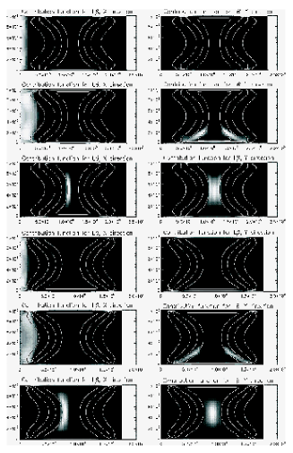
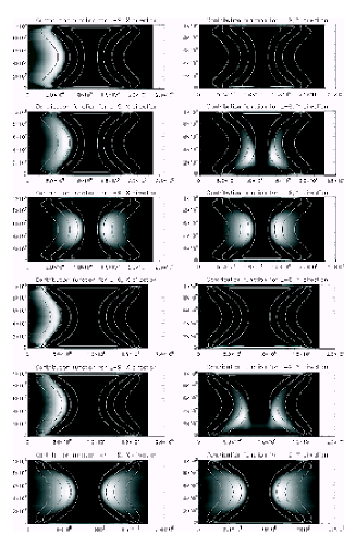
Figure 10.: Contribution functions along and across the field lines showing the formation depths of the hydrogen Lyman $\beta$ (left two columns) and Lyman 9 (right two columns). Two different models are displayed (twice three rows). In each part, the first row corresponds to the line center, the second one to the peak wavelength and the third one to the wing. Left columns refer to the direction along the field lines ($x$-direction), while right columns to the direction across the field ($y$-direction). The temperature contours are also drawn showing two quite different PCTR’s. The line core of Lyman $\beta$ is formed at the surface of the 2D thread (at the highest temperatures), the peaks deeper and in the line wing we can see the central parts of the structure. The Lyman 9 line is optically thinner and thus the thread more transparent in all wavelengths allowing the diagnostics of deeper layers. Note the different scales in both directions, in reality the “fibril” projected onto solar disk is much more stretched.

9 RMHD Simulations

Equation (3) gives the 1D MHS equilibrium of the KS-type. In order to see how the cool and dense plasma structure can evolve in the magnetic field under the action of Lorentz and gravity forces, Bárta et al. (2007) solved numerically the system of compressible one-fluid MHD equations in a 2D vertical plane, starting with the dense and cool blob (a thread in 3D) representing a thread of the filament fine structure surrounded by the gravitationally stratified, constant-temperature hot corona. The initial magnetic field has only a horizontal component. At the very beginning the plasma blob starts to fall down, the internal electric current is induced inside it which generates the restoring Lorenz force. Due to the inertial mass the blob overshoots the (global) equilibrium point and an upward-directed Lorentz force prevails over the gravity turning the movement of the blob up. The system starts to oscillate but due to the numerical viscous term the oscillations are damped. After several oscillations the system is practically relaxed and in the MHS equilibrium. The evolution of the system at four subsequent times is shown in Fig. 11. These first simulations will now be replaced by fully 3D modeling which will also include the 3D radiative transfer. The latter is necessary to determine the ionization state of the plasma and its radiation losses.

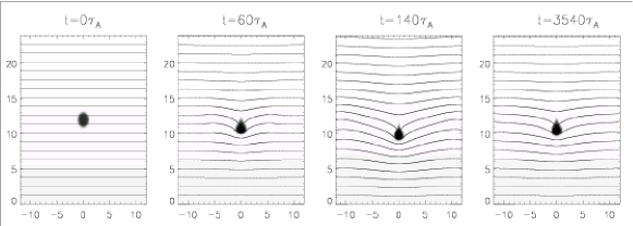
Figure 11.: A sequence of four snapshots of the prominence fine-structure evolution according to the MHD system of equations. The simulation is carried out in the dimensionless units; lengths are expressed in the initial thread half-width $L_{\rm t}$, times in the units of Alfvén transit time $\tau_{\rm A}=L_{\rm t}/v_{\rm A}$. Recalculated for reasonable coronal conditions (coronal temperature $T_{\rm c}=2\times 10^{6}$K, coronal gravitation length scale $L_{\rm g}=6\times 10^{9}$ cm) we get $L_{\rm t}\approx 1200$ km, $\tau_{\rm A}\approx 20$ s. Thus the thread characteristic dimension is $\approx 2500$ km and the final (relaxed) state in the last frame is reached after almost 20 hours.

10 Comments on Magnetic Dips

Any analysis of 2D images or movies can lead to misinterpretations just due to the lack of information on fully 3D structural and dynamical pattern. As an example we will mention here again the scenario of counter-streaming (Zirker et al. (1998) or Lin et al. (2003)). A close inspection of high-resolution H$\alpha$ movies (see them on CD enclosed to the Solar Physics Vol. 216) reveals that dark fine-strucure blobs (rather than long threads) move on relatively short paths, although sometimes in opposite directions. These motions don’t resemble at all flows along long magnetic fluxtubes, but rather a kind of oscillations. Quite interestingly, when watching the TRACE movies of similar prominences, one clearly sees sideway oscillations of small blobs which, projected on the disk, would probably resemble the kind of motions seen on SST movies (projected blobs seen in H$\alpha$ and TRACE 195 Å  are shown in Fig. 5). However, these blobs visible on TRACE movies form very frequently the quasi-vertical threads also shown in Fig. 1 and Fig. 2 and thus, according to our discussion above, they should represent plasma condensations hanging in a dipped magnetic field which seems to oscillate in the corona. This scenario is, however, quite different from that of Lin et al. (2003) (flows along long fluxtubes without any dips).

Another observational support for dips being located along the prominence spine is the fact that the H$\alpha$ absorbing fibrils are concentrated along the spine and we typically don’t see any significant absorption further away from the spine. This seems to indicate that there are no such flows which could be detected along the whole magnetic arcade which is of course much wider than the width of the spine. Even H$\alpha$ images or movies taken out of the line center don’t show such a pattern.

Actually there should be no principal controversy between low-$\beta$ dip models and gravity-induced dip models. Yet there are no time-dependent simulations of how the plasma is condensed in a dipped field and how this may evolve leading to an enhancement of the plasma density and thus its weight which, eventually, will modify the magnetic structure of the dip. Existing time-dependent simulations of prominence condensations assume an initial shape of the magnetic loop and this is not changed during simulations even when the mass loading at the loop top increases. Static models of dips which neglect the prominence weight (fff extrapolations) can reasonably well reproduce the large-scale distribution of dips and this has proven to be a quite novel approach. On the other hand, static models of gravity-induced dips have been developed to understand the local magnetic topology of a dip and its thermodynamic and radiative properties. These two approaches should not be in conflict, but rather complementary: provided that the plasma-$\beta$ is large enough, the weight effects should be added to initially fff-dips. This is a challenge for future prominence modeling. As discussed above, today the actual values of plasma beta are still very uncertain and thus various configurations are possible. An important diagnostics test would be the quantitative modeling of the H$\alpha$ contrast of fine-structure fibrils located along the filament spines. This contrast, which certainly increases with increasing spatial resolution of new telescopes, is due to the absorption of the background radiation in the H$\alpha$ line (the scattering contribution to the source function is typically small). It has to be modeled in 3D fibril geometry which requires realistic estimate of the mass loading. An example of how this can be handled was given recently by Heinzel & Anzer (2006), who used some kind of (2+1)D models to demonstrate the theoretical H$\alpha$ contrast of gravity-induced magnetic dips as projected against the solar disk. A few examples are shown in Fig. 12, where the fibril models do exhibit a significant stretching in the direction of the magnetic field and this resembles real dark fibrils as seen e.g., in Fig. 3.

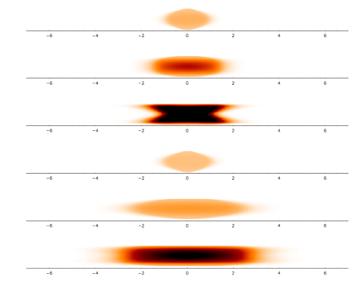
Figure 12.: (2+1)D models of H$\alpha$ fibrils. Six 2D thread models are shown with different mass loadings and magnetic-field strengths. From Heinzel & Anzer (2006).

11 Conclusions

To conclude this review, let us go again back to Secchi (1877). In his book Le Soleil one can read: “Les protubérances se présentent sous des aspects si bizarres et si capricieux qu’il est absolument impossible de les décrire avec quelque exactitude.” After 130 years, this still seems to be the case.

Acknowledgments.

I am very grateful to my colleagues and collaborators for many useful discussions which helped me to prepare this review and to others from SOC and LOC for a nice meeting. In particular, I am indebted to Uli Anzer and Rob Rutten for reading the manuscript and suggesting several improvements. This work was done in the frame of the ESA-PECS project No. 98030. I also acknowledge travel support from the ESMN.

References

- Anzer (2002) Anzer, U. 2002, in Proc. 10th Solar Physics Meeting, ESA SP-506, 389
- Anzer & Heinzel (1999) Anzer, U., & Heinzel, P. 1999, A&A, 349, 974
- Anzer & Heinzel (2005) Anzer, U., & Heinzel, P. 2005, ApJ, 622, 714
- Anzer & Heinzel (2007) Anzer, U., & Heinzel, P. 2007, A&A, in press
- Athay et al. (1983) Athay, R.G., Querfeld, C., Smartt, R., Landi Degl’Innocenti, E., & Bommier, V. 1983, Solar Phys., 89, 3
- Auer & Paletou (1994) Auer, L.H., & Paletou, F. 1994, A&A, 285,675
- Aulanier & Démoulin (1998) Aulanier, G., & Démoulin, P. 1998, A&A, 329, 1125
- Aulanier & Démoulin (2003) Aulanier, G., & Démoulin, P. 2003, A&A, 402, 769
- Aulanier & Schmieder (2002) Aulanier, G., & Schmieder, B. 2002, A&A, 386, 1106
- Aulanier et al. (2000) Aulanier, G., Srivastava, N., & Martin, S. 2000, ApJ, 543, 447
- Avrett (2007) Avrett, E.H., 2007, in P. Heinzel, I. Dorotovič, R. J. Rutten (eds.), The Physics of Chromospheric Plasmas, ASP Conf. Ser. 368, 81
- Aznar Cuadrado et al. (2003) Aznar Cuadrado, R., Andretta, V., Teriaca, L., & Kucera, T.A. 2003, Mem. S. A. It., 74, 611
- Bárta et al. (2007) Bárta, M., Anzer, U., Heinzel, P., & Karlický, M. 2007, in preparation
- Bommier et al. (1994) Bommier, V., Leroy, J.-L., Landi Degl’Innocenti, E., & Sahal-Bréchot, S. 1994, Solar Phys., 154, 231
- Chae et al. (2005) Chae, J., Moon, Y.J., & Park, Y.D. 2005, ApJ., 626, 574
- Cirigliano et al. (2004) Cirigliano, D., Vial, J.-C., & Rovira, M. 2004, Solar Phys., 223, 95
- Engvold (1976) Engvold, O. 1976, Solar Phys., 49, 283
- Engvold (1998) Engvold, O. 1976, in Proc. IAU Coll. 167, New Perspectives on Solar Prominences, ed. D. Webb, D. Rust & B. Schmieder, ASP Conf. Ser., 150, 23
- Engvold (2004) Engvold, O. 2004, in Proc. IAU Symp. No. 223, ed. A.V. Stepanov & E. Benevolenskaya, (Cambridge: Cambridge Univ. Press), 187
- Fontenla & Rovira (1984) Fontenla, J.M., & Rovira, M. 1985, Solar Phys. 96, 53
- Fontenla et al. (1990) Fontenla, J., Avrett, G., Loeser, R. 1990, ApJ, 355, 700
- Fontenla et al. (1996) Fontenla, J., Rovira, M., Vial, J.-C., & Gouttebroze, P. 1996, ApJ, 466, 496
- Gouttebroze (2004) Gouttebroze, P. 2004, A&A, 413, 733
- Gouttebroze (2007) Gouttebroze, P. 2007, A&A, in press
- Gouttebroze & Labrosse (2000) Gouttebroze, P., & Labrosse, N. 2000, Solar Phys., 196, 349
- Gouttebroze et al. (1993) Gouttebroze, P., Heinzel, P., & Vial, J.-C. 1993, A&AS, 99, 513
- Gunár et al. (2007) Gunár, S., Heinzel, P., & Anzer, U. 2007, A&A, 463, 737
- Heasly & Mihalas (1976) Heasley, J.N., & Mihalas, D. 1978, ApJ, 205, 273
- Heasley & Milkey (1978) Heasley, J.N. & Milkey, R.W. 1978, ApJ, 221, 677
- Heinzel (1989) Heinzel, P. 1989, in Proc. IAU Coll. 117, Hvar Obs. Bull. 13, 279
- Heinzel (1995) Heinzel, P. 1995, A&A, 299, 563
- Heinzel & Anzer (1998) Heinzel, P., & Anzer, U. 1998, Solar Phys., 179, 75
- Heinzel & Anzer (1999) Heinzel, P., & Anzer, U. 1999, Solar Phys., 184, 103
- Heinzel & Anzer (2001) Heinzel, P., & Anzer, U. 2001, A&A, 375, 1082
- Heinzel & Anzer (2005) Heinzel, P., & Anzer, U. 2005, in Solar Magnetic Phenomena, ed. A. Hanslmeier, A. Veronig & M. Messerotti, Astrophys. Space Sci. Lib., 320 (Springer: Dordrecht), 115
- Heinzel & Anzer (2006) Heinzel, P., & Anzer, U. 2006, ApJ, 643, L65
- Heinzel & Avrett (2007) Heinzel, P. & Avrett, G. 2007, in preparation
- Heinzel & Vial (1992) Heinzel, P., & Vial, J.-C. 1992, Proc. ESA Workshop on Solar Physics and Astrophysics at Interferometry Resolution, ESA SP-348, 57
- Heinzel et al. (2005) Heinzel, P., Anzer, U., & Gunár, S. 2005, A&A, 442, 331
- Heinzel et al. (2006) Heinzel, P., Schmieder, B., & Vial, J.-C. 2006, Proc. SOHO 17 – 10 years of SOHO and Beyond, ESA SP-617 (CD-ROM)
- Heinzel et al. (2001) Heinzel, P., Schmieder, B., Vial, J.-C., & Kotrč, P. 2001, A&A, 370, 281
- Karpen et al. (2006) Karpen, J.T., Antiochos, S.K., & Klimchuk, J.A. 2006, ApJ, 637, 531
- Kippenhahn & Schlüter (1957) Kippenhahn, R., & Schlüter, A. 1957, Z. Astrophys., 43, 36
- Kuperus & Raadu (1974) Kuperus, M., & Raadu, M.A. 1974, A&A, 31, 189
- Leroy (1989) Leroy, J.-L. 1989, in Dynamics and Structure of Quiescent Solar Prominences, ed. E.R. Priest, Astrophys. Space Sci. Lib., 150, 77
- Leroy et al. (1983) Leroy, J.-L., Sahal-Bréchot, S., & Bommier, V. 1983, Solar Phys., 83, 135
- Lin et al. (2003) Lin, Y., Engvold, O., & Wiik, J.E. 2003, Solar Phys. 216, 109
- López Ariste & Aulanier (2007) López Ariste, A., & Aulanier, G. 2007, in P. Heinzel, I. Dorotovič, R. J. Rutten (eds.), The Physics of Chromospheric Plasmas, ASP Conf. Ser. 368, 291
- Low & Petrie (2005) Low, B.C., & Petrie, G.J.D. 2005, ApJ, 626, 551
- Mihalas et al. (1978) Mihalas, D., Auer, L.H., & Mihalas, B.W. 1978, ApJ, 220, 1001
- Morozhenko (1984) Morozhenko, N. N. 1984, Spectrophotometric investigations of quiescent solar prominences (Naukova dumka: Kiev)
- Paletou (1995) Paletou, F. 1995, A&A, 302, 587
- Parenti et al. (2004) Parenti, S., Vial, J.-C., & Lemaire, P. 2004, Solar Phys., 220, 61
- Parenti et al. (2005) Parenti, S., Vial, J.-C., & Lemaire, P. 2005, A&A, 443, 685
- Patsourakos & Vial (2002) Patsourakos, S., & Vial, J.-C. 2002, Solar Phys., 208, 253
- Pécseli & Engvold (2000) Pécseli, H., & Engvold, O. 2000, Solar Phys., 194, 73
- Poland & Anzer (1971) Poland, A.I., & Anzer, U. 1971, Solar Phys., 19, 401
- Poland & Mariska (1988) Poland, A.I., & Mariska, J.T. 1988, in Dynamics and Structure of Solar Prominences, ed. J.L. Ballester & E.R. Priest (Université des Illes Baléares), 133
- Poland & Tandberg-Hanssen (1983) Poland, A.I., & Tandberg-Hanssen, E. 1983, Solar Phys., 84, 63
- Priest (1990) Priest, E.R. 1990, in Proc. IAU Coll. 117, ed. V. Ruždjak & E. Tandberg-Hanssen, Lecture Notes in Physics, 363 (Springer-Verlag: Berlin), 150
- Rutten (1999) Rutten, R.J. 1999, in Proc. 3rd Advances in Solar Physics Euroconference: Magnetic Fields and Oscillations, ed. B. Schmieder, A. Hofmann & J. Staude, ASP Conf. Ser., 184 (ASP: San Francisco), 181
- Secchi (1877) Secchi, A. 1877, Le Soleil (Gauthier-Villars: Paris)
- Schmieder et al. (2007) Schmieder, B., Gunár, S., Heinzel, P., & Anzer, U. 2007, Solar Phys., in press
- Schmieder et al. (2004) Schmieder, B., Lin, Y., Heinzel, P., & Schwartz, P. 2004, Solar Phys., 221, 297
- Stellmacher & Wiehr (2005) Stellmacher, G., & Wiehr, E. 2005, A&A, 431, 1059
- Tandberg-Hanssen (1995) Tandberg-Hanssen, E. 1995, The Nature of Solar Prominences (Kluwer: Dordrecht)
- van Ballegooijen (2004) van Ballegooijen, A.A. 2004, ApJ, 612, 519
- Vial (1982) Vial, J.-C. 1982, ApJ, 254, 780
- Vial (1998) Vial, J.-C. 1998, in Proc. IAU Coll. 167, New Perspectives on Solar Prominences, ed. D. Webb, D. Rust, & B. Schmieder, ASP Conf. Ser., 150, 175
- Vial (2006) Vial, J.-C. 2006, Proc. SOHO 17 – 10 years of SOHO and Beyond, ESA SP-617 (CD-ROM)
- Vial et al. (2007) Vial, J.-C., Ebadi, H., & Ajabshirizadeh, A. 2007, Solar Phys., in press
- Vial et al. (1989) Vial, J.-C., Rovira, M., Fontenla, J., & Gouttebroze, P. 1989, in Proc. IAU Coll. 117, Hvar Obs. Bull. 13, 347
- Wiehr et al. (2007) Wiehr, E., Stellmacher, G., & Hirzberger, J. 2007, Solar Phys., in press
- Wiik et al. (1999) Wiik, J.E., Dammasch, I.E., Schmieder, B., & Wilhelm, K. 1999, Solar Phys., 187, 405
- Yakovkin & Zel’dina (1975) Yakovkin, N.A., & Zel’dina, M. Yu. 1975, Solar Phys. 45, 319
- Zharkova (1989) Zharkova, V.V. 1989, in Proc. IAU Coll. 117, Hvar Obs. Bull., 13, 331
- Zirker & Koutchmy (1990) Zirker, J.B., & Koutchmy, S. 1990, Solar Phys., 127, 109
- Zirker & Koutchmy (1991) Zirker, J.B., & Koutchmy, S. 1991, Solar Phys., 131, 107
- Zirker et al. (1998) Zirker, J.B., Engvold, O., & Martin, S.F. 1998, Nature, 396, 440