Knots in the Skyrme-Faddeev model

Abstract

The Skyrme-Faddeev model is a modified sigma model in three-dimensional space, which has string-like topological solitons classified by the integer-valued Hopf charge. Numerical simulations are performed to compute soliton solutions for Hopf charges up to sixteen, with initial conditions provided by families of rational maps from the three-sphere into the complex projective line. A large number of new solutions are presented, including a variety of torus knots for a range of Hopf charges. Often these knots are only local energy minima, with the global minimum being a linked solution, but for some values of the Hopf charge they are good candidates for the global minimum energy solution. The computed energies are in agreement with Ward’s conjectured energy bound.

1 Introduction

Over thirty years ago Faddeev suggested [4] that in three-dimensional space the $O(3)$ sigma model, modified by the addition of a Skyrme term, should have interesting string-like topological solitons stabilized by the integer-valued Hopf charge. Ten years ago substantial interest was generated by the first attempts at a numerical construction of such solitons [5, 6] and the suggestion that minimal energy solitons might take the form of knots [5]. This conjecture has been confirmed by numerical results, which demonstrate that the minimal energy soliton with Hopf charge seven is a trefoil knot [1]. Substantial numerical investigations by several authors [5, 6, 1, 7, 8, 14] has produced a comprehensive analysis of solitons with Hopf charges from one to seven, and it appears that the global energy minima have now been identified for these charges, together with several other stable soliton solutions that correspond to local energy minima.

For Hopf charges five and six the minimal energy solitons form links, but so far the charge seven solution remains the only known knot, even including local energy minima. It is therefore currently unknown whether this charge seven trefoil knot is the only knotted solution or if there are many other knots, perhaps of various types, which arise for higher Hopf charges. It is this question which is addressed in the present paper. Solitons with Hopf charges up to sixteen are constructed numerically and it is found that a variety of torus knots exist at various Hopf charges. Often these knots are only local energy minima, with the global minimum being a link, but for some values of the Hopf charge it appears that a knot is a good candidate for the global minimum energy solution.

One of the difficulties in extending previous numerical studies to higher Hopf charges is that, even at low charges, there are a number of local energy minima with large capture basins. This makes it difficult to fully explore the landscape of local energy minima and hence determine the global minimum, with the severity of the problem generally increasing as the charge increases. To overcome this problem an analytic ansatz is employed which uses rational maps from the three-sphere into the complex projective line. Although this ansatz does not provide any exact solutions, it does allow the construction of reasonable initial conditions for any torus knot for a large range of charges, plus a wide selection of links and unknots. It is therefore possible to start at a variety of locations in field configuration space, in particular where one suspects that a local energy minimum might be close by, and explore the energy landscape around this point. Not only is this a fruitful approach for finding new solutions, but it can also be used to provide strong evidence that a solution of a particular type does not exist, by starting with an initial condition approximating this configuration and demonstrating that it changes dramatically under energy relaxation.

An analysis is made of the new knotted and linked solutions and some understanding is obtained regarding the charges at which particular knots are likely to exist.

2 The Skyrme-Faddeev model and low charge solitons

The Skyrme-Faddeev model involves a map $\mbox{\boldmath$\phi$}:\hbox{\mybb R}^{3}\mapsto S^{2},$ which is realized as a real three-component vector $\mbox{\boldmath$\phi$}=(\phi_{1},\phi_{2},\phi_{3}),$ of unit length, $\mbox{\boldmath$\phi$}\cdot\mbox{\boldmath$\phi$}=1.$ As this paper is concerned only with static solutions then the model can be defined by its energy

$$E=\frac{1}{32\pi^{2}\sqrt{2}}\int\partial_{i}\mbox{\boldmath$\phi$}\cdot\partial_{i}\mbox{\boldmath$\phi$}+\frac{1}{2}(\partial_{i}\mbox{\boldmath$\phi$}\times\partial_{j}\mbox{\boldmath$\phi$})\cdot(\partial_{i}\mbox{\boldmath$\phi$}\times\partial_{j}\mbox{\boldmath$\phi$})\ d^{3}x,$$ (2.1)

where the normalization is chosen for later convenience. The first term in the energy is that of the usual $O(3)$ sigma model and the second is a Skyrme term, required to provide a balance under scaling and hence allow solitons with a finite non-zero size.

Finite energy boundary conditions require that the field tends to a constant value at spatial infinity, which is chosen to be $\mbox{\boldmath$\phi$}(\infty)=(0,0,1)={\bf e}_{3}.$ This boundary condition compactifies space to $S^{3},$ so that the field becomes a map $\mbox{\boldmath$\phi$}:S^{3}\mapsto S^{2}.$ Such maps are classified by $\pi_{3}(S^{2})=\hbox{\mybb Z},$ so there is an integer-valued topological charge $Q,$ the Hopf charge, which gives the soliton number. Unlike most theories with topological solitons, the topological charge is not a winding number or degree of a mapping. Rather, it has a geometrical interpretation as a linking number of field lines, as follows. Generically, the preimage of a point on the target two-sphere is a closed loop (or a collection of closed loops) in the three-sphere domain obtained from the compactification of $\hbox{\mybb R}^{3}.$ Two loops obtained as the preimages of any two distinct points on the target two-sphere are linked exactly $Q$ times, where $Q$ is the Hopf charge.

The Hopf charge can be written as the integral over the three-sphere domain of a charge density, but this density is non-local in the field $\mbox{\boldmath$\phi$},$ as the following construction demonstrates. Let $\omega$ denote the area two-form on the target two-sphere and let $F=\mbox{\boldmath$\phi$}^{*}\omega$ be its pull-back under $\phi$ to the domain three-sphere. The triviality of the second cohomology group of the three-sphere implies that $F$ is an exact two-form, say $F=dA.$ The Hopf charge is then given by integrating the Chern-Simons three-form over the three-sphere as

$$Q=\frac{1}{4\pi^{2}}\int_{S^{3}}F\wedge A.$$ (2.2)

The energy bound

$$E\geq c\,Q^{3/4},\quad\mbox{where}\quad c=\left(\frac{3}{16}\right)^{3/8}\approx 0.534$$ (2.3)

has been proved [12, 9], and it is known that the fractional power is optimal [10], though it is expected that the above value of the constant $c$ is not. Motivated by a study of the Skyrme-Faddeev model on a three-sphere with a finite radius, together with an analogy with the Skyrme model, Ward has conjectured [13] that the above energy bound holds with the value $c=1$ (hence the choice of normalization factor for the energy in (2.1)), but this has not been proven. As discussed shortly, the current energy values known for low charge solitons are in good agreement with Ward’s conjectured energy bound, and later it will be demonstrated that the energies for higher charge solitons are too.

The simplest examples of Hopf solitons are axially symmetric and their qualitative features may be described as follows. First, consider the model (2.1) defined in two-dimensional space, so that the boundary conditions now result in a compactification of space from $\hbox{\mybb R}^{2}$ to $S^{2}.$ The field is then a map $\mbox{\boldmath$\phi$}:S^{2}\mapsto S^{2}$ and is classified by an integer $m\in\hbox{\mybb Z}=\pi_{2}(S^{2}),$ which is the usual winding number familiar from the $O(3)$ sigma model itself. Strictly speaking, in order to have two-dimensional solitons with a finite size in this model then a potential term must also be included, upon which the two-dimensional solitons are known as baby Skyrmions [11], but this aspect is not crucial for the discussion here. Returning to the three-dimensional model, then a toroidal field configuration can be formed by embedding the two-dimensional soliton in the normal slice to a circle in space. The two-dimensional soliton has an internal phase and this can be rotated through an angle $2\pi n,$ as it travels around the circle once, where $n\in\hbox{\mybb Z}$ counts the number of twists. A field configuration of this type has Hopf charge $Q=nm,$ and it will be denoted by ${\cal A}_{n,m},$ so the first subscript labels the number of twists and the second is the winding number of the two-dimensional soliton forming the loop.

The minimal energy $Q=1$ soliton is of the type ${\cal A}_{1,1}$ and has been studied numerically by a number of authors [6, 5, 1, 7, 14] using different algorithms. Taken together, these results suggest that the charge one soliton has an energy of around $E=1.21,$ and this is part of a general pattern where the minimal energy soliton exceeds Ward’s conjectured bound by around $20\%.$ The numerical computations reported in this paper produce a charge one energy of $E=1.204,$ and hence appear to underestimate the energy by an amount of the order of $1\%.$ For low charge solitons this accuracy could be improved by increasing the resolution of the numerical grid, but it is computationally too expensive to increase the resolution for all the large number of simulations reported here for large charges. Moreover, although the energy is a slight underestimate for a given soliton solution, the relative energies between two given solutions are much more accurate than this (changing grid resolutions and sizes suggests an accuracy of around $0.1\%$) and it is more important to preserve the relative energies than the absolute energy of any single solution.

The details of the numerical computations are similar to those of Ref.[1], and full details of the related numerical code used to study Skyrmions can be found in Ref.[2]. Briefly, a finite difference scheme is employed with a lattice spacing $\Delta x=0.1$ on a grid containing $(151)^{3}$ lattice points, with the field fixed to the vacuum value $\mbox{\boldmath$\phi$}={\bf e}_{3}$ on the boundary of the grid; this is preferable to other methods of dealing with the finite volume simulation domain, such as the one used in Ref.[1] which led to a more substantial underestimate of energies, though again relative energies had a high accuracy. The energy minimization algorithm proceeds by evolving second order in time dynamics and periodically removing kinetic energy from the system whenever the potential energy of the system begins to increase. It is based on the approach employed in Ref.[1], but is computationally more efficient since the second order dynamics is derived from the kinetic term of the sigma model only, rather than the full kinetic term determined from the Lorentz invariant Lagrangian associated with the energy (2.1). This subtle difference leads to a more efficient algorithm since the leading term in the evolution equations is now diagonal, so a costly matrix inversion can be avoided.

A sensible definition of the position of a soliton is to identify where the field is as far as possible from the vacuum field. A Hopf soliton is therefore string-like, since the soliton’s position is defined to be the closed loop (or collection of loops) corresponding to the preimage of the point $\mbox{\boldmath$\phi$}=-{\bf e}_{3}=(0,0,-1),$ which is antipodal to the vacuum value on the target two-sphere. To visualize a field configuration this position curve is plotted, though for clarity a tube around this position is displayed, given by an isosurface of the form $\phi_{3}=-1+\nu,$ where generally the value $\nu=0.2$ is chosen. If a pictorial representation of the Hopf charge is also required then a second preimage curve can also be plotted (again as a tube), and the linking number of these two curves inspected. There is no natural choice for this second preimage value (${\bf e}_{3}$ is not a very useful choice) and in this paper when a second preimage curve is displayed it corresponds to the point $\mbox{\boldmath$\phi$}=(\sqrt{2\mu-\mu^{2}},0,-1+\mu)$ where $\mu=0.1.$ In what follows this curve will be referred to as the linking curve, and since $\mu$ is relatively small then the linking curve remains reasonably close to the position curve, making it fairly easy to inspect the linking number.

In Figure 1 the position (light tube) and linking (dark tube) curves are displayed for the known lowest energy solitons with Hopf charges from one to seven. Given the large number of numerical simulations performed by different groups it seems reasonably certain that these are the minimal energy solitons for these charges. The energies of these solutions will be discussed later, and as mentioned above they are generally around $20\%$ above Ward’s conjectured bound, but for now it is the structure of the solutions that is of primary interest, and this is reviewed below.

The solutions with charges one and two are both axially symmetric, and are of the type ${\cal A}_{1,1}$ and ${\cal A}_{2,1}$ respectively [5, 6], with one and two twists of the linking curve around the position curve clearly visible. There is a solution of the form ${\cal A}_{1,2}$ [13, 14, 7] but it has an energy around $13\%$ above that of the minimal charge two soliton. This solution has the interpretation of two $Q=1$ solitons stacked one above the other, preserving the axial symmetry.

The charge three soliton is basically of the type ${\cal A}_{3,1}$ but the axial symmetry is broken as the position curve is bent [1], so it will be denoted by $\widetilde{\cal A}_{3,1}$ to emphasize that the structure is deformed. There is an axial solution of the type ${\cal A}_{n,1}$ for any integer $n,$ but for $n>2$ this solution is unstable to a coiling instability [1]; a well-known phenomenon in other settings such as twisted elastic rods. The $Q=4$ soliton is of the type ${\cal A}_{2,2},$ [8, 13], and may be thought of as two $Q=2$ solitons stacked one above the other. For both $Q=4$ and $Q=5$ there are also bent solutions [1], similar to the charge three soliton, and therefore denoted $\widetilde{\cal A}_{4,1}$ and $\widetilde{\cal A}_{5,1},$ but unlike the $Q=3$ case, both these solutions are only local energy minima, with energies around $2\%$ and $4\%$ above the global minimum, respectively.

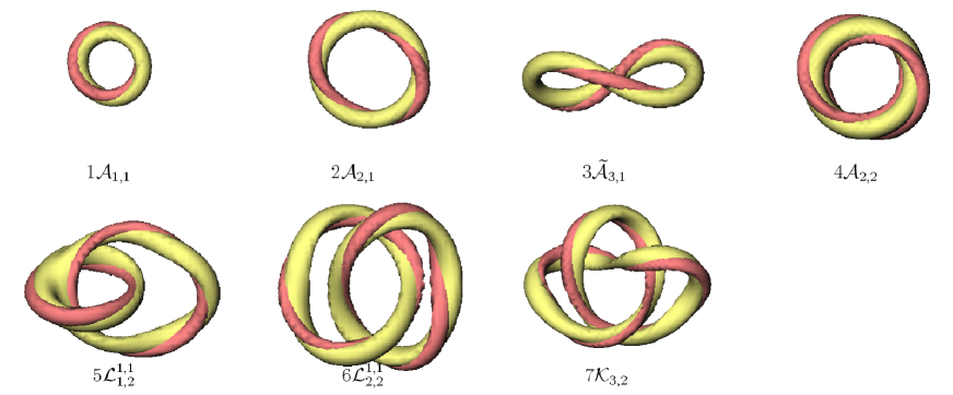
Figure 1: The position (light tube) and linking (dark tube) curves for the known lowest energy solitons with Hopf charges $1\leq Q\leq 7.$

The minimal energy charge five soliton provides the first example of a link, that is, a solution in which the position curve contains two or more disconnected components. It consists of a charge one soliton and a charge two soliton which are linked once [8], with the result that each of these solitons gains an additional unit of linking number to make a total of five. To denote a link of this type the notation ${\cal L}_{1,2}^{1,1}$ will be used, where the subscripts label the charges of the components of the links and the superscript above each subscript counts the extra linking number of that component, due to its linking with the others. Hence the total charge is the sum of the subscripts plus superscripts. The charge six soliton is similar to that of charge five, but now both components of the link have charge two [1], so using the above notation it is written as ${\cal L}_{2,2}^{1,1}.$

Finally, the charge seven soliton is the first (and so far only) example of a knot [1]. The position curve is a trefoil knot, which has a self-linking or crossing number of three (the crossing number of a knot is not an invariant and its use in this paper refers to the minimal crossing number over all presentations). An examination of the linking curve in Figure 1 confirms that it twists around the position curve four times as the knot is traversed, so the Hopf charge is indeed seven, being the sum of the crossing number plus the number of twists. Any field configuration of a trefoil knot will be denoted by ${\cal K}_{3,2},$ which refers to the fact that the trefoil knot is also the $(3,2)$-torus knot (see the following section for more information regarding torus knots). Note that this notation does not display the Hopf charge of the configuration, which is determined by the twist number as well as the crossing number, but this should not cause any confusion in what follows. Of course, for knots and links, as well as for unknot configurations, the precise conformation of the position curve is important in determining the energy, not just its topological type, but its knotted or linked structure is an important feature in classifying the solution. Thus, for example, the $Q=7$ trefoil knot displayed in Figure 1 is not as symmetric as its typical knot theory presentation, and it is significant that the energy is lowered by breaking the possible cyclic $C_{3}$ symmetry.

Having reviewed the known results for low charge solitons and introduced the notation used to label their structural type, it is time to turn to the main questions addressed in this paper. Given the variety of solutions which appear, even at low charges, it is difficult to make a confident prediction of the kind of behaviour that might arise at higher charges. In particular, an interesting open question is whether more knot solitons appear at higher charge, and if so what types of knots arise and are they local or global minima? It could have been the case that the charge seven trefoil knot was the only knot soliton, though in this paper it will be shown that this is far from true. Also, it would be useful to have at least a qualitative understanding of the fact that $Q=7$ is the lowest charge at which a knot first appears, and desirable to be able to estimate the charges at which other knots might exist.

In this section it has been mentioned briefly that at each charge there are often local minima in addition to the global minimum, and it is expected that the number of local minima generally increases with the charge. As noted in the introduction, these local minima can have large capture basins, making it difficult to fully explore the space of solutions. For any relaxation computation this makes the choice of initial conditions a crucial issue. In particular, it is not obvious how to construct a variety of reasonably low-energy initial field configurations for all Hopf charges. One family of configurations are the axial fields ${\cal A}_{n,1},$ which are all unstable for $n>2.$ However, even for charges as low as four, initial conditions which use small perturbations of these unstable solutions get trapped in local minima. One successful approach for low charges involves constructing links by hand [7, 8], using a numerical cut-and-paste technique where various numerical field configurations are sewn together in different parts of the simulation grid to create a linked field with a given Hopf charge. Although this approach was the first method to successfully yield the global minima at charges four and five, it becomes more cumbersome for larger charges and is not applicable for creating knot initial conditions; it is also not very elegant mathematically, but this is perhaps not a serious criticism. Another set of initial conditions that have been used [8] are based on the fields ${\cal A}_{n,m},$ with $m>1,$ though these fields tend to have relatively large energies and therefore require quite long simulation times (except for the low charge examples of ${\cal A}_{1,2}$ and ${\cal A}_{2,2}).$ In the following section an analytic ansatz is presented that yields reasonable field configurations for a variety of charges and describes all torus knots plus a wide range of links, in addition to fields of the type ${\cal A}_{n,m}.$ The key ingredient of the ansatz involves a rational map from the three-sphere into the complex projective line. The ansatz allows the construction of initial conditions corresponding to a variety of locations in field configuration space; in particular, configurations can be created which are reasonably close to suspected local energy minima. This approach substantially reduces the computational effort required to explore the energy landscape and makes it feasible to study knots and links for quite large charges.

3 Rational maps, torus knots and links

Torus knots are classified by a pair $(a,b)$ of coprime positive integers with $a>b.$ A knot is a torus knot if it lies on the surface of a torus, in which case the integers $a$ and $b$ count the number of times that the knot winds around the two cycles of the torus. The simplest example is the trefoil knot, which is the $(3,2)$-torus knot and has three crossings. In the standard knot catalogue notation it is $3_{1},$ where the number refers to the crossing number of the knot and the subscript labels its position in the knot catalogue. Other torus knots which will be of interest in this paper include the $(5,2)$-torus knot, also known as Solomon’s seal knot, which has five crossings (knot $5_{1}$ in the catalogue), and the $(4,3)$-torus knot which has crossing number eight (knot $8_{19}$ in the catalogue). In general the $(a,b)$-torus knot has crossing number $C=a(b-1).$

Denote by ${\cal K}_{a,b}$ any field configuration in which the position curve is an $(a,b)$-torus knot. Such a field configuration will have Hopf charge $Q=C+T,$ where $C=a(b-1)$ is the knot crossing number and the integer $T$ counts the number of times that the linking curve twists around the position curve (only situations where the orientation is such that $T$ is non-negative will be of relevance here). The main aim of this section is to construct fields of type ${\cal K}_{a,b}$ for a large range of charges $Q.$

The first step is to recall the standard description [3] of a torus knot as the intersection of a complex algebraic curve with the three-sphere. Consider $(Z_{1},Z_{0})\in\hbox{\mybb C}^{2}$ and the unit three-sphere $S^{3}\subset\hbox{\mybb C}^{2}$ given by $|Z_{1}|^{2}+|Z_{0}|^{2}=1.$ Then the intersection of this three-sphere with the complex algebraic curve $Z_{1}^{a}+Z_{0}^{b}=0$ is indeed the $(a,b)$-torus knot.

To use the above description to produce a field configuration, the spatial coordinates $(x_{1},x_{2},x_{3})\in\hbox{\mybb R}^{3}$ are mapped to the unit three-sphere via a degree one spherically equivariant map. Explicitly,

$$(Z_{1},Z_{0})=((x_{1}+ix_{2})\frac{\sin f}{r},\cos f+i\frac{\sin f}{r}x_{3}),$$ (3.1)

where $r^{2}=x_{1}^{2}+x_{2}^{2}+x_{3}^{2}$ and the profile function $f(r)$ is a monotonically decreasing function of the radius $r$, with boundary conditions $f(0)=\pi$ and $f(\infty)=0.$ The precise form of this function will be specified shortly.

A Riemann sphere coordinate $W,$ is used on the target two-sphere of the field $\mbox{\boldmath$\phi$},$ determined via stereographic projection as

$$W=\frac{\phi_{1}+i\phi_{2}}{1+\phi_{3}}.$$ (3.2)

With these definitions, then constructing a map $\mbox{\boldmath$\phi$}:\hbox{\mybb R}^{3}\mapsto S^{2}$ is equivalent to specifying $W(Z_{1},Z_{0}),$ that is, $W:S^{3}\mapsto\hbox{\mybb C}\hbox{\mybb P}^{1},$ a map from the three-sphere to the complex projective line. This map will be taken to be a rational map, which means that $W=p/q,$ where both $p$ and $q$ are polynomials in the variables $Z_{1}$ and $Z_{0}.$

For an $(a,b)$-torus knot the mapping is chosen to have the form

$$W=\frac{p}{q}=\frac{Z_{1}^{\alpha}Z_{0}^{\beta}}{Z_{1}^{a}+Z_{0}^{b}},$$ (3.3)

where $\alpha$ is a positive integer and $\beta$ is a non-negative integer. A map of this form has the correct boundary conditions at spatial infinity, since as $r\rightarrow\infty$ then $(Z_{1},Z_{0})\rightarrow(0,1)$ and, because $\alpha>0,$ this gives $W\rightarrow 0,$ which is the stereographic projection of the point $\mbox{\boldmath$\phi$}=(0,0,1)={\bf e}_{3}.$ Furthermore, the position curve is the preimage of the point $-{\bf e}_{3},$ which corresponds to $W=\infty,$ and hence is given by $q=0=Z_{1}^{a}+Z_{0}^{b}.$ As the coordinates $(Z_{1},Z_{0})$ automatically lie on the unit three-sphere then the position curve is the $(a,b)$-torus knot, for all values of $\alpha$ and $\beta.$

The Hopf charge of the map determined by (3.3) is given by the cross ratio

$$Q=\alpha b+\beta a.$$ (3.4)

To see this note that a rational map

$$W:S^{3}\mapsto\hbox{\mybb C}\hbox{\mybb P}^{1},\quad\mbox{given\ by}\quad W(Z_{1},Z_{0})=\frac{p(Z_{1},Z_{0})}{q(Z_{1},Z_{0})},$$ (3.5)

has a natural extension to a map

$$(p,q):\hbox{\mybb B}^{4}\subset\hbox{\mybb C}^{2}\mapsto\hbox{\mybb C}^{2},\quad\mbox{given\ by}\quad(p(Z_{1},Z_{0}),q(Z_{1},Z_{0})).$$ (3.6)

Here $\hbox{\mybb B}^{4}$ denotes the 4-ball with boundary $S^{3},$ and is obtained by replacing the constraint $|Z_{1}|^{2}+|Z_{0}|^{2}=1$ by the inequality $|Z_{1}|^{2}+|Z_{0}|^{2}\leq 1.$ The map $(p,q)$ is between manifolds of the same dimension and has a degree, defined by counting preimages of a generic point of the target space, weighted by the signs of the Jacobian. As all the other mappings involved in the ansatz have degree one, and the standard Hopf map $(p,q)\mapsto p/q$ is employed, then the Hopf charge $Q$ of the combined mapping is equal to the degree of the mapping $(p,q).$ Furthermore, as the mapping $(p,q)$ is holomorphic then the sign of the Jacobian of all generic preimage points is positive, so the degree is simply the number of preimages.

For the mapping $(p,q)$ given by (3.3) take the generic point in target space to be $(\epsilon,0),$ so the Hopf charge is the number of solutions of the equation $(Z_{1}^{\alpha}Z_{0}^{\beta},Z_{1}^{a}+Z_{0}^{b})=(\epsilon,0).$ Writing $Z_{0}$ in terms of $Z_{1}$ from the first component of this equation and substituting into the second component yields the polynomial equation $Z_{1}^{\alpha b+\beta a}=(-1)^{\beta}\epsilon^{b},$ which clearly has $Q=\alpha b+\beta a$ solutions, as stated.

For any $(a,b)$-torus knot the above ansatz can be used to construct a field configuration of the type ${\cal K}_{a,b}$ with Hopf charge $Q,$ providing there are integers $(\alpha,\beta),$ with $\alpha$ positive and $\beta$ non-negative, for which $Q=\alpha b+\beta a.$ For example, in the case of the trefoil knot then $(a,b)=(3,2)$ hence any $Q>3$ can be obtained. In fact a trefoil knot with $Q=3$ can also be obtained by interchanging the roles of $Z_{1}$ and $Z_{0},$ but a field of this type is not relevant, as will be made clear later. Note that for some values of $Q,$ and fixed $(a,b),$ there are multiple solutions for $(\alpha,\beta).$ These multiple solutions produce qualitatively similar fields, in that both describe the same $(a,b)$-torus knot position curve, and the linking curve twists the same number of times around the position curve; though the distribution of twist may vary. In examples where such multiple solutions were used as initial conditions, the energy relaxation algorithm produced identical final results for all choices.

Recall that a profile function $f(r)$ needs to be specified, satisfying the boundary conditions $f(0)=\pi$ and $f(\infty)=0.$ In fact, these are the correct boundary conditions in an infinite domain but in the finite domain used for numerical simulations the last boundary condition needs to be replaced by $f=0$ at the boundary of the numerical grid. As the ansatz is only used to provide initial conditions then most reasonable monotonic functions will suffice. The simulations discussed in this paper were performed on a cubic grid of side-length $2L,$ that is, $-L\leq x_{i}\leq L,$ where $2L=15.$ A simple linear profile function was used, given by $f(r)=\pi(L-r)/L,$ for $r\leq L$ and zero otherwise. For a given rational map one could aim to minimize the energy of the ansatz over all profile functions, but this has not been attempted for reasons discussed shortly.

As an illustration of the use of the ansatz, consider an approximation to the minimal energy $Q=7$ trefoil knot. To construct a field ${\cal K}_{3,2}$ with $Q=2\alpha+3\beta=7,$ requires $(\alpha,\beta)=(2,1),$ resulting in the map $W=Z_{1}^{2}Z_{0}/(Z_{1}^{3}+Z_{0}^{2}).$ The field generated from this rational map is displayed in Figure 2a, where both the position and linking curves are shown. It is clear from this figure that the field has similar qualitative features to the minimal energy soliton, in that it is a trefoil knot with four twists. The main qualitative difference is that the ansatz produces a more symmetric field, having a cyclic $C_{3}$ symmetry. This symmetry is obvious from the form of the rational map, as a rotation by $120^{\circ}$ around the $x_{3}$-axis corresponds to the transformation $Z_{1}\mapsto e^{2\pi i/3}Z_{1},$ upon which the rational map changes by only a phase; which is simply an action of the global $O(2)$ symmetry on target space.

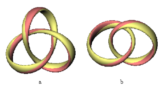
Figure 2: The position (light tube) and linking (dark tube) curves for initial conditions created using the rational map ansatz: (a) $Q=7$ trefoil knot; (b) $Q=6$ link ${\cal L}_{2,2}^{1,1}.$

Using the above field as the initial condition for an energy relaxation simulation yields the minimal energy soliton very quickly, and certainly requires far less computational resources than computing the solution from a perturbed axial configuration. Note that, in practice, the cyclic $C_{3}$ symmetry is slightly broken by the cubic numerical grid, and in particular its boundary, so an explicit symmetry breaking perturbation is not required. In examples discussed later, where initial conditions have a cyclic $C_{4}$ symmetry, then the configuration is created with a slight displacement from the centre of the grid to again slightly break any exact symmetry.

As mentioned above, the profile function could be optimized to find the minimal energy configuration, for a given rational map, but this has not been attempted. As with the above example, generally the ansatz is more symmetric than the relaxed solution, so it is not expected that a good estimate of the energy can be obtained in this way. It might be possible to improve the approximation to a quantitative level by minimizing over families of rational maps, which include symmetry breaking terms, rather than using the rational maps in this paper; chosen to be the simplest with the correct qualitative features. In this case it would be worthwhile to also minimize the profile function, but as the minimization problem couples the rational map and the profile function together then this is not a simple numerical task. In fact, this numerical problem appears to have about the same level of difficulty as performing energy relaxation via full field simulations. As the energy relaxation code produces a solution very quickly and efficiently from the simple ansatz, then there appears little need to try and improve upon it. The profile function could be adjusted to a minimal extent, for example, by including parameters to set the scale and thickness of the knot, but again this has not been necessary.

So far only knot initial conditions have been considered, but the ansatz can also be used to construct a variety of unknots and links by choosing suitable rational maps. For example, axial fields of the form ${\cal A}_{n,m}$ are generated by a rational map $W=Z_{1}^{n}/Z_{0}^{m}.$

Links correspond to rational maps in which the curve determined by the denominator is reducible. The torus knot maps with $(a,b)$ coprime degenerate to links if $(a,b)$ are not coprime. As an example, links of the type ${\cal L}_{n,n}^{1,1}$ (which have Hopf charge $Q=2n+2$) are derived from the rational map

$$W=\frac{Z_{1}^{n+1}}{Z_{1}^{2}-Z_{0}^{2}}=\frac{Z_{1}^{n}}{2(Z_{1}-Z_{0})}+\frac{Z_{1}^{n}}{2(Z_{1}+Z_{0})},$$ (3.7)

where the partial fraction decomposition reveals the charges of the constituent links by comparison with the axial maps. The $Q=6$ field constructed using the rational map $(\ref{links})$ with $n=2$ is displayed in Figure 2b. As can be seen from this figure, the field is qualitatively similar to the minimal energy $Q=6$ soliton, which is of the type ${\cal L}_{2,2}^{1,1}.$ More examples of rational maps associated to linked configurations will appear in the following section.

	initial
Q	$\downarrow$
	final
	${\cal K}_{3,2}$
5	$\downarrow$
	${\cal L}_{1,2}^{1,1}$
	${\cal K}_{3,2}$
6	$\downarrow$
	${\cal L}_{2,2}^{1,1}$
	${\cal K}_{3,2}$	${\cal L}_{2,3}^{1,1}$
7	$\downarrow$	$\downarrow$
	${\cal K}_{3,2}$	${\cal K}_{3,2}$
	${\cal L}_{3,3}^{1,1}$	${\cal L}_{2,2}^{2,2}$	${\cal L}_{4,2}^{1,1}$	${\cal K}_{5,2}$	${\cal K}_{3,2}$
8	$\downarrow$	$\downarrow$	$\downarrow$	$\downarrow$	$\downarrow$
	${\cal L}_{3,3}^{1,1}$	${\cal L}_{3,3}^{1,1}$	${\cal L}_{3,3}^{1,1}$	${\cal L}_{3,3}^{1,1}$	${\cal K}_{3,2}$
	${\cal L}_{1,1,1}^{2,2,2}$	${\cal K}_{4,3}$	${\cal K}_{3,2}$	${\cal K}_{5,2}$	${\cal L}_{2,3}^{2,2}$	${\cal L}_{3,4}^{1,1}$
9	$\downarrow$	$\downarrow$	$\downarrow$	$\downarrow$	$\downarrow$	$\downarrow$
	${\cal L}_{1,1,1}^{2,2,2}$	${\cal L}_{1,1,1}^{2,2,2}$	${\cal K}_{3,2}$	${\cal K}_{3,2}$	${\cal K}_{3,2}$	${\cal K}_{3,2}$
	${\cal L}_{1,1,2}^{2,2,2}$	${\cal K}_{4,3}$	${\cal L}_{3,3}^{2,2}$	${\cal L}_{5,3}^{1,1}$	${\cal K}_{5,2}$	${\cal K}_{3,2}$
10	$\downarrow$	$\downarrow$	$\downarrow$	$\downarrow$	$\downarrow$	$\downarrow$
	${\cal L}_{1,1,2}^{2,2,2}$	${\cal L}_{1,1,2}^{2,2,2}$	${\cal L}_{3,3}^{2,2}$	${\cal L}_{3,3}^{2,2}$	${\cal L}_{3,3}^{2,2}$	${\cal K}_{3,2}$
	${\cal K}_{4,3}$	${\cal K}_{5,2}$	${\cal K}_{7,2}$	${\cal K}_{3,2}$
11	$\downarrow$	$\downarrow$	$\downarrow$	$\downarrow$
	${\cal L}_{1,2,2}^{2,2,2}$	${\cal K}_{5,2}$	${\cal L}_{3,4}^{2,2}$	${\cal K}_{3,2}$
	${\cal K}_{5,3}$	${\cal K}_{3,2}$	${\cal K}_{5,2}$	${\cal K}_{7,2}$
12	$\downarrow$	$\downarrow$	$\downarrow$	$\downarrow$
	${\cal L}_{2,2,2}^{2,2,2}$	${\cal K}_{4,3}$	${\cal K}_{5,2}$	${\cal L}_{4,4}^{2,2}$
	${\cal K}_{3,2}$	${\cal K}_{5,3}$	${\cal K}_{5,2}$	${\cal K}_{7,2}$
13	$\downarrow$	$\downarrow$	$\downarrow$	$\downarrow$
	${\cal K}_{4,3}$	${\cal X}_{13}$	${\cal K}_{5,2}$	${\cal L}_{3,4}^{3,3}$
	${\cal K}_{4,3}$	${\cal K}_{5,3}$	${\cal K}_{3,2}$
14	$\downarrow$	$\downarrow$	$\downarrow$
	${\cal K}_{4,3}$	${\cal K}_{5,3}$	${\cal K}_{5,2}$
	${\cal K}_{5,3}$	${\cal K}_{4,3}$	${\cal K}_{3,2}$
15	$\downarrow$	$\downarrow$	$\downarrow$
	${\cal X}_{15}$	${\cal L}_{1,1,1}^{4,4,4}$	${\cal K}_{5,3}$
	${\cal K}_{4,3}$	${\cal L}_{1,1,1,1}^{3,3,3,3}$	${\cal K}_{3,2}$
16	$\downarrow$	$\downarrow$	$\downarrow$
	${\cal X}_{16}$	${\cal X}_{16}$	${\cal X}_{16}$

Table 1: Initial conditions and final solutions.

$Q$	type	$E$	$E/Q^{3/4}$
1	${\cal A}_{1,1}$	1.204	1.204
2	${\cal A}_{2,1}$	1.967	1.170
3	$\widetilde{\cal A}_{3,1}$	2.754	1.208
4	${\cal A}_{2,2}$	3.445	1.218
5	${\cal L}_{1,2}^{1,1}$	4.095	1.225
6	${\cal L}_{2,2}^{1,1}$	4.650	1.213
7	${\cal K}_{3,2}$	5.242	1.218
8	${\cal L}_{3,3}^{1,1}$	5.821	1.224
8	${\cal K}_{3,2}$	5.824	1.224
9	${\cal L}_{1,1,1}^{2,2,2}$	6.360	1.224
9	${\cal K}_{3,2}$	6.385	1.229
10	${\cal L}_{1,1,2}^{2,2,2}$	6.905	1.228
10	${\cal L}_{3,3}^{2,2}$	6.923	1.231
10	${\cal K}_{3,2}$	6.973	1.240
11	${\cal L}_{1,2,2}^{2,2,2}$	7.391	1.224
11	${\cal K}_{5,2}$	7.502	1.242
11	${\cal L}_{3,4}^{2,2}$	7.533	1.247
11	${\cal K}_{3,2}$	7.614	1.261
12	${\cal L}_{2,2,2}^{2,2,2}$	7.833	1.215
12	${\cal K}_{4,3}$	7.857	1.219
12	${\cal K}_{5,2}$	8.070	1.252
12	${\cal L}_{4,4}^{2,2}$	8.093	1.255
13	${\cal K}_{4,3}$	8.272	1.208
13	${\cal X}_{13}$	8.462	1.236
13	${\cal K}_{5,2}$	8.574	1.252
13	${\cal L}_{3,4}^{3,3}$	8.633	1.261
14	${\cal K}_{4,3}$	8.761	1.210
14	${\cal K}_{5,3}$	8.807	1.217
14	${\cal K}_{5,2}$	9.124	1.261
15	${\cal X}_{15}$	9.290	1.219
15	${\cal L}_{1,1,1}^{4,4,4}$	9.404	1.234
15	${\cal K}_{5,3}$	9.408	1.234
16	${\cal X}_{16}$	9.769	1.221

Table 2: Solution types and energies.

4 Higher charge solitons

In this section the results of a large number of energy minimization simulations are presented. Hopf charges up to sixteen are studied, with initial conditions consisting of a variety of links and knots, created using the rational map ansatz discussed above.

Table 1 summarizes the simulations performed, by listing the type of each initial condition together with the type of the resulting final solution, obtained from the energy minimization algorithm. In Table 2 the types and energies of the known lowest energy solutions, plus some local energy minima, are presented for $1\leq Q\leq 16,$ ordered by increasing energies. Also given in Table 2 are the energies divided by Ward’s conjectured bound, $E/Q^{3/4},$ from which it can be seen that the minimal energy solution is consistently around $20\%$ above the conjectured bound. The values of $E/Q^{3/4}$ are plotted in Figure 3 using a notation that identifies the different torus knots as follows. White circles denote configurations which do not contain knots, that is, either unknots or links. The symbols denoting knots are triangles for ${\cal K}_{3,2}$, diamonds for ${\cal K}_{5,2},$ squares for ${\cal K}_{4,3}$ and stars for ${\cal K}_{5,3}.$ Configurations denoted by black circles will be discussed shortly.

Figure 3: The ratio of the energy to the conjectured bound, that is, $E/Q^{3/4},$ as a function of Hopf charge $Q$ for a variety of solutions: unknots and links (white circles); ${\cal K}_{3,2}$ (triangles); ${\cal K}_{5,2}$ (diamonds); ${\cal K}_{4,3}$ (squares); ${\cal K}_{5,3}$ (stars); links which are not resolved (black circles).

The present study has produced 26 new solutions with $8\leq Q\leq 16.$ The position curves for each of these is displayed in Figure 4, but for clarity the linking curves are not shown, although they have been examined to confirm the correct linking number identifications. Each plot is labeled by its charge and type, with energies increasing first from left to right and then top to bottom.

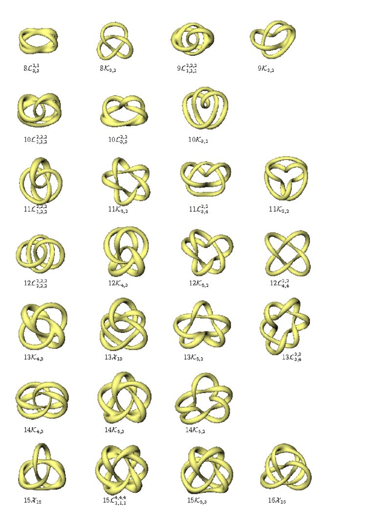
Figure 4: The position curves for a variety of solutions with Hopf charge $8\leq Q\leq 16.$ Each plot is labeled by its charge and type.

First of all, consider trefoil knots, that is, solutions which have the form ${\cal K}_{3,2}.$ As mentioned earlier, the $Q=7$ minimal energy soliton has this form and is obtained from the related rational map initial condition. This is encoded in Table 1 as the process ${\cal K}_{3,2}\rightarrow{\cal K}_{3,2}.$ The entry to the right of this one in Table 1 reveals that the same trefoil knot solution is also obtained from the linked initial condition ${\cal L}_{2,3}^{1,1}.$

There are no trefoil knots with $Q<7.$ Evidence supporting this is presented in Table 1 for $Q=5$ and $Q=6,$ where it is seen that in both cases initial conditions of the form ${\cal K}_{3,2}$ result in the linked minimal energy solutions, which are ${\cal L}_{1,2}^{1,1}$ and ${\cal L}_{2,2}^{1,1}$ respectively. A reasonable interpretation of these results is that for $Q<7$ the number of twists $T=Q-3$ is too low, given the preferred length of the soliton in a trefoil knot arrangement. In other words, the twist per unit length is too low to be an energetically efficient distribution of the Hopf charge between crossing and twisting. A more detailed discussion of this aspect will be given later, when general torus knots will be considered. Note that, in particular, there is no trefoil knot solution in which there is no twist, which corresponds to $Q=3,$ and was the original suggestion for a knot soliton [5].

Table 1 shows that there are also trefoil knot solutions for $Q=8,9,10,11$ and in each case they are obtained from rational map initial conditions of the type ${\cal K}_{3,2}.$ For $Q=9$ the trefoil solution is also obtained from a variety of other initial conditions, including links and the torus knot ${\cal K}_{5,2};$ this last process ${\cal K}_{5,2}\rightarrow{\cal K}_{3,2}$ provides an example of knot transmutation, where Solomon’s seal knot deforms into a trefoil knot. In Figure 4 a comparison of the plots $8{\cal K}_{3,2},9{\cal K}_{3,2},10{\cal K}_{3,2},11{\cal K}_{3,2}$, emphasizes that the conformation of the knot is important, with each of these trefoils having a very different structure to the others. In particular, as the number of twists increases the knot increasingly contorts and bends, in a manner similar to that seen in the axial solutions ${\cal A}_{n,1},$ where for $n=3$ the response to the twist is to lower the energy by bending to break the axial symmetry. As mentioned earlier, for $n=4,5$ there are similar bent solutions, which are local minima, where the deformation increases with $n.$ Trefoil knots therefore appear to follow a similar pattern, with a minimal number of twists, that is 4, required for existence and increasingly deformed solutions existing with slightly larger twists than the minimal value.

The triangles in Figure 3, and the associated energy values in Table 2, show that the ratio of the energy to the bound steadily increases for the trefoil solutions as the charge increases. It is therefore not surprising that for a large enough charge, which happens to be $Q=12,$ a trefoil solution fails to exist. Table 1 confirms that a $Q=12$ initial condition of the type ${\cal K}_{3,2}$ produces a solution which is not a trefoil knot, and will be discussed later. The triangles in Figure 3 also confirm that only for the minimal value $Q=7$ is the trefoil knot the global minimum energy solution, and in all other cases a trefoil is only a local energy minimum. However, for $Q=8$ the trefoil knot energy is extremely close to the lowest energy found, which is a linked solution ${\cal L}_{3,3}^{1,1}.$ In fact the energies differ by less than $0.1\%,$ which is probably smaller than the accuracy of the computations, so in this case it is difficult to make a definitive statement regarding which (if any) is the global minimum.

In Ref.[1] a linked solution of the type ${\cal L}_{2,2}^{2,2}$ was reported, but this appears to be an artefact of that study being at the limit of computational feasibility for computing resources available at that time. A configuration of this type does appear during a relaxation procedure, but after further relaxation it changes its type. Moreover, an initial condition of the type ${\cal L}_{2,2}^{2,2}$ can be constructed using the rational map

$$W=\frac{Z_{1}^{4}}{Z_{1}^{4}-Z_{0}^{2}}=\frac{Z_{1}^{2}}{2(Z_{1}^{2}-Z_{0})}+\frac{Z_{1}^{2}}{2(Z_{1}^{2}+Z_{0})},$$ (4.1)

and, as seen from Table 1, the relaxation yields a solution of a different type, namely the linked solution ${\cal L}_{3,3}^{1,1}.$ It therefore now seems unlikely that a charge eight stable solution exists of the type ${\cal L}_{2,2}^{2,2}.$ Note that the rational map $(\ref{map8})$ describes a link in which both components are linked twice with each other, and this is because the irreducible factors of the denominator are terms like $(Z_{1}^{2}-Z_{0}),$ rather than terms like $(Z_{1}-Z_{0}),$ where the latter corresponds to only single links between any two components. The partial fraction decomposition in $(\ref{map8})$ reveals that each component of the link has charge two, by once again reading off the power of the numerator.

For a given fixed charge there is nothing to prevent multiple trefoil knot solutions which differ in their conformations and energies, but no evidence for this phenomenon has been found. For example, Table 1 shows that the $Q=9$ trefoil knot is produced from (at least) four different types of initial condition, but in each case the resulting trefoil solution is the same one with an identical conformation. This is the case for all the solutions described in this paper, that is, when a particular solution is obtained from various initial conditions it is always in the same conformation, so its charge and type are sufficient to distinguish it from any other solution.

As the trefoil knot solutions for $Q=9,10,11$ are clearly only local energy minima then it remains to describe the candidates found for the global minima for these charges. In fact for all three of these charges, and also for $Q=12,$ the lowest energy solutions found have a similar form, which is a link with three components. The simplest case, $Q=9,$ is displayed in Figure 4 as plot $9{\cal L}_{1,1,1}^{2,2,2},$ and as this label suggests there are three components to the link, each of which has charge one and links once with each of the other two components. An initial condition of the type ${\cal L}_{1,1,1}^{2,2,2}$ with $Q=9$ is obtained from the rational map

$$W=\frac{Z_{1}^{3}}{Z_{1}^{3}-Z_{0}^{3}},$$ (4.2)

and quickly relaxes to the minimal energy solution with the same type. The initial condition has a more planar arrangement of the three components than the final solution, and the initial cyclic $C_{3}$ symmetry is also broken, as can be seen from plot $9{\cal L}_{1,1,1}^{2,2,2},$ in Figure 4. Note from Table 1 that this 3-component link is also obtained from a knotted initial condition of the type ${\cal K}_{4,3},$ but that out of the six $Q=9$ initial conditions used, four lead to the higher energy trefoil knot solution. This is evidence that supports the fact that minimal energy solutions may not be the easiest to find; hence the need to employ the variety of starting configurations used in this study.

The minimal energy solutions with $Q=10,11,12$ are similar to the minimal $Q=9$ solution and correspond to increasing one, two and finally all three, of the charge one components to charge two. In other words they have the forms ${\cal L}_{1,1,2}^{2,2,2},{\cal L}_{1,2,2}^{2,2,2}$ and ${\cal L}_{2,2,2}^{2,2,2}$ respectively. These solutions are displayed in Figure 4 and in each case there is an associated rational map of the same type. Table 1 shows that they can all be obtained from the relaxation of certain torus knot initial conditions.

So far the only knot solutions discussed have been trefoil knots. As the torus knot with the lowest crossing number after the trefoil is the $(5,2)$-torus knot, then this is the most likely candidate to appear next as a soliton solution. Table 1 reveals that an initial condition of the type ${\cal K}_{5,2}$ does not yield a solution of this type for $Q=8,9,10,$ but it does for $Q=11.$ The $Q=11$ solution is displayed in Figure 4 as plot $11{\cal K}_{5,2}.$ It is only a local energy minimum, despite the fact that it is lower in energy than the $Q=11$ trefoil knot. There are also solutions of the type ${\cal K}_{5,2}$ for $Q=12,13,14$ and the pattern mirrors that of the trefoil knots, in that the ratio of the energy to the bound steadily increases with the charge; see the diamonds in Figure 3.

At $Q=12$ a solution of the type ${\cal K}_{4,3}$ appears (see Figure 4 plot $12{\cal K}_{4,3}$) and its energy is just above that of the minimal energy ${\cal L}_{2,2,2}^{2,2,2}$ link, though substantially lower than that of the ${\cal K}_{5,2}$ solution. Solutions of the type ${\cal K}_{4,3}$ also exist for $Q=13$ and $Q=14,$ and for these two charges they are the lowest energy solutions found. The excess energy above the bound is also reasonably low, so these two solutions are good candidates for the global minima at $Q=13$ and $Q=14.$ The squares in Figure 3 denote the ratio of the energy to the bound for ${\cal K}_{4,3}$ solutions, from which it can be seen that (unlike the other torus knots) the lowest charge at which this knot appears is not the one that is closest to the conjectured bound.

At $Q=13$ a solution exists (see Figure 4 plot $13{\cal X}_{13}$) which is denoted by ${\cal X}_{13}$ because there is no unambiguous interpretation as a particular link or knot. This is due to the fact that a definition of a link or knot requires the position curve not to self-intersect, but there is nothing to prevent this in the field theory. For the ${\cal X}_{13}$ solution then either the position curve self-intersects exactly, or there are parts of the curve that are so close together that they can not be resolved with the numerical accuracy currently employed. Some of the lower charge solutions presented earlier may also appear to self-intersect, for example the $Q=5$ solution displayed in Figure 1, but in all these lower charge solutions the apparent self-intersection can be resolved by reducing the thickness of the tube plotted around the position curve, together with a careful consideration of continuity.

If there are no self-intersection points in the solution ${\cal X}_{13}$ then there are two possibilities for the configuration type, depending on how this self-intersection point is resolved. The first possibility is the link ${\cal L}_{1,2,2}^{2,3,3},$ and the second is a link with two components, where one of the components is a trefoil knot with five twists and the second component is approximately axial with a single twist. The latter resolution is essentially an intertwining of the charge eight trefoil knot solution with the charge one solution.

The lowest energy solitons found for $Q=15$ and $Q=16$ are denoted by ${\cal X}_{15}$ and ${\cal X}_{16}$ respectively, and also have points which can not be distinguished from self-intersection points, as seen from plots $15{\cal X}_{15}$ and $16{\cal X}_{16}$ in Figure 4. In each case there is a resolution into a link with two components where one of the components is a trefoil knot. The conformation of both the knot and unknot components in these cases strongly suggests that this is the correct resolution, if indeed one is required. The $Q=16$ solution is the easiest to identify and consists of the charge eight trefoil knot intertwined with the minimal energy charge two solution, where the conformation of both components is very similar to that of the components in isolation. A field with the correct qualitative behaviour to describe this resolution is given by the rational map

$$W=\frac{Z_{1}^{5}+Z_{1}^{2}Z_{0}^{2}+Z_{1}Z_{0}^{3}}{Z_{0}Z_{1}^{3}+Z_{0}^{3}}=\frac{Z_{1}Z_{0}^{2}}{Z_{1}^{3}+Z_{0}^{2}}+\frac{Z_{1}^{2}}{Z_{0}}.$$ (4.3)

Initial conditions generated using this rational map quickly leads to the solution ${\cal X}_{16}$ under energy relaxation.

The solution ${\cal X}_{15}$ is similar to the solution ${\cal X}_{16},$ except that the resolution involves the charge seven trefoil knot, rather than the charge eight trefoil knot. The energies of the solutions of type ${\cal X}_{n}$ are represented by black circles in Figure 3.

Note that $Q=16$ is the lowest charge in which a link with four components each linking all the others might exist. However, as seen in Table 1, an initial condition of the type ${\cal L}_{1,1,1,1}^{3,3,3,3}$ relaxes to the ${\cal X}_{16}$ solution.

The final torus knot solitons presented in this paper are of the type ${\cal K}_{5,3}$ and exist for $Q=14$ and $Q=15,$ but in both cases these solutions are only local energy minima. The energies of these solutions are represented by stars in Figure 3.

In summary, it has been shown that there are a variety of torus knot solitons at various Hopf charges. For example, at $Q=14$ three different torus knot solutions have been obtained. Most of the knot solitons found are only local energy minima, but in some cases they are good candidates for the global minimum.

Figure 5: String length (circles) as a function of charge $Q$ for several solitons, together with the expected growth behaviour $\gamma Q^{3/4}$ (curve).

For a string-like soliton it is expected that one of the contributions to the energy should have an interpretation in terms of the string length. As the soliton energy grows like $Q^{3/4}$ then this suggests that the string length should have a similar growth. In Figure 5 the string length is plotted (circles) for several solitons, including examples of both knots and links. Also shown is a curve with the expected power growth, $\gamma Q^{3/4},$ where $\gamma$ has been computed by a least squares fit to be $\gamma=7.86.$ This plot demonstrates a reasonable agreement with the expected $Q^{3/4}$ dependence of the string length. The greatest discrepancy from the expected string length occurs for the $Q=15$ link ${\cal L}_{1,1,1}^{4,4,4},$ which is much longer than expected. However, note that this solution has an abnormally large ratio of linking to twist number, with the contribution to the Hopf charge from linking being four times that from twisting. The solution with the next largest ratio of linking to twist is the $Q=9$ link ${\cal L}_{1,1,1}^{2,2,2},$ where linking contributes twice as much as twisting, and the length of this solution is also a bit above the expected value. It therefore appears that solutions which link much more than they twist require an increased string length to minimize energy.

Recall from the earlier discussion of knot solitons, that there appears to be a critical twist, below which knot solitons of a particular type do not exist. A twist below the critical value seems to be an energetically inefficient distribution of the Hopf charge between twisting and crossing. For twists just above the critical value a knot solution continues to exist but as the twist increases further then again the distribution between twisting and crossing becomes inefficient, but this time due to too much twisting.

A naive approximation is to assume that for all solutions there is a universal optimum twist per unit length. Taking this optimum value from that of the $Q=1$ soliton, and using the fact that the string length grows like $Q^{3/4},$ this suggests that an optimum value for the number of twists is approximately $T\approx Q^{3/4}.$ For a knot with crossing number $C$ this gives $C=Q-T\approx Q-Q^{3/4}.$ Using this assumption, a knot with crossing number $C$ is predicted to be energetically efficient at an integer charge near to the real value $Q_{*},$ which is defined as the solution of the equation $Q_{*}-Q_{*}^{3/4}=C.$ For example, for the trefoil knot $C=3$ and therefore $Q_{*}=7.56,$ which roughly agrees with the $Q=7$ and $Q=8$ trefoils being closest to the energy bound. For $C=5$ then $Q_{*}=11.07$ and this explains why the $Q=11$ knot ${\cal K}_{5,2}$ is closest to the bound. For $C=8$ then $Q_{*}=16,$ so the naive approximation overestimates the most efficient value, which is seen to be $Q=13$ for the ${\cal K}_{4,3}$ knot. There are clearly more subtle effects at work than the simple naive constant twist rate assumed in this calculation, but it does seem to produce numbers which are in the right ballpark, suggesting that it captures some qualitative aspects of knot energetics.

5 Conclusion

The results presented in this paper reveal that there are many low-energy knot solitons of various types, for a range of Hopf charges, together with increasingly complicated linked solitons. The qualitative features of these solutions can be replicated using an ansatz involving rational maps from the three-sphere to the complex projective line, and futhermore this provides a good supply of initial conditions for numerical relaxation simulations. The complicated nature of the problem means that it is difficult to be certain that the global minimal energy solitons have been found, but certainly some good candidates have been presented, whose energies agree well with the expected values based on an earlier conjectured bound.

The rational map ansatz allows the construction of any torus knot initial condition, but it is not clear how to extend this to non-torus knots. All the knot solutions found so far are torus knots, and it is unknown whether the lack of non-torus knot solitons is a result of not having suitable initial conditions, or whether there is some energetic reason to favour torus knots. For example, the figure eight knot has four crossings and hence a soliton with this form might be expected with a charge around $Q=9.$ As seen from Table 1, quite a few initial conditions have been employed for $Q=9$ and $Q=10,$ and no such solution has been found. It remains an open problem to understand the absence (or otherwise) of non-torus knots.

Finally, given that there are many knot and link solitons then it would be useful if there was an approximate string model that could, even qualitatively, reproduce the field theory results. It has been shown that the string length has the expected behaviour with Hopf charge, so it is plausible that there may be an approximate description based on a string energy that includes contributions from properties of the string such as its length, twist and writhe, together with relevant interaction terms.

References

- [1] R. A. Battye and P. M. Sutcliffe, Knots as stable soliton solutions in a three-dimensional classical field theory, Phys. Rev. Lett. 81, 4798 (1998); Solitons, links and knots, Proc. R. Soc. Lond. A455, 4305 (1999).
- [2] R. A. Battye and P. M. Sutcliffe, Skyrmions, fullerenes and rational maps, Rev. Math. Phys. 14, 29 (2002).
- [3] E. Brieskorn and H. Knörrer, Plane algebraic curves, Birkhäuser-Verlag (1986).
- [4] L. D. Faddeev, Quantization of solitons, Princeton preprint IAS-75-QS70 (1975).
- [5] L. Faddeev and A. J. Niemi, Stable knot-like structures in classical field theory, Nature 387, 58 (1997).
- [6] J. Gladikowski and M. Hellmund, Static solitons with nonzero Hopf number, Phys. Rev. D56, 5194 (1997).
- [7] J. Hietarinta and P. Salo, Faddeev-Hopf knots: dynamics of linked un-knots, Phys. Lett. B451, 60 (1999).
- [8] J. Hietarinta and P. Salo, Ground state in the Faddeev-Skyrme model, Phys. Rev. D62, 081701(R) (2000).
- [9] A. Kundu and Yu. P. Rybakov, Closed-vortex-type solitons with Hopf index, J. Phys. A15, 269 (1982).
- [10] F. Lin and Y. Yang, Existence of energy minimizers as stable knotted solitons in the Faddeev model, Commun. Math. Phys. 249, 273 (2004).
- [11] B. M. A. G. Piette, B. J. Schroers and W. J. Zakrzewski, Multisolitons in a two-dimensional Skyrme model, Z. Phys. C65, 165 (1995).
- [12] A. F. Vakulenko and L. V. Kapitanski, Stability of solitons in in the nonlinear -model, Dokl. Akad. Nauk USSR 246, 840 (1979).
- [13] R. S. Ward, Hopf solitons on and , Nonlinearity 12, 241 (1999).
- [14] R. S. Ward, The interaction of two Hopf solitons, Phys. Lett. B473, 291 (2000).