Effect of inelastic collisions on multiphonon Raman scattering in graphene

Abstract

We calculate the probabilities of two- and four-phonon Raman scattering in graphene and show how the relative intensities of the overtone peaks encode information about relative rates of different inelastic processes electrons are subject to. If the most important processes are electron-phonon and electron-electron scattering, the rate of the latter can be deduced from the Raman spectra.

Introduction.— Collisions of Dirac electrons are qualitatively different from those of electrons in conventional metals: energy and momentum conservation leave no phase space for relaxation of a quasiparticle excited above the Dirac vacuum. Electron collisions in graphene and related compounds continue to be a subject of theoretical studies Guinea96 ; Rubio ; DasSarma . Thus, any experimental information on collisions of Dirac electrons would be extremely valuable. However, to experimentally separate contributions from different mechanisms to electron lifetime is a hard task. The present work suggests a way to separate electron-phonon and electron-electron contributions to the electron lifetime by analyzing Raman spectra.

Raman spectrum of graphene consists of distinct peaks corresponding to different optical phonon branches as well as their overtones. Thus, Raman scattering measurements represent a powerful experimental tool for studying phonon modes, as well as their interaction with electrons (since electronic excitations are involved in Raman scattering as intermediate states). Indeed, electron-phonon interaction and Raman scattering in graphene has attracted a great deal of interest, both experimental Ferrari ; Gupta ; Graf ; Pisana ; Jun and theoretical Lazzeri ; Guinea . Here we show how even more information can be extracted from Raman spectra.

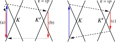
Figure 1: Schematic representation of the role of electron dispersion (Dirac cones, shown by solid lines) in Raman scattering: (a) one-phonon $G$ peak, (b) impurity-assisted one-phonon $D$ peak, (c) two-phonon $D^{*}$ peak. Vertical solid arrows represent interband electronic transitions accompanied by photon absorption or emission (photon wave vector is neglected), dashed arrows represent phonon emission, the horizontal dotted arrow represents impurity scattering.

Qualitative picture.— Photon wave vector is negligible, so momentum conservation requires that Raman scattering on one intervalley phonon must be impurity-assisted [process (b) in Fig. 1, giving rise to the so-called $D$ Raman peak]. $D$ peak is absent in the experimental Raman spectrum of graphene Ferrari , so impurity scattering is negligible in these samples, and is disregarded hereafter.

Looking at the intermediate electronic states (Fig. 1), we notice that for one-phonon scattering [processes (a), (b)] at least one intermediate state must be virtual, since energy and momentum conservation cannot be satisfied simultaneously. For the two-phonon scattering [process (c)] all electronic states can be real. We emphasize the qualitative difference between the fully resonant process (c) and the double-resonant ThomsenReich process (b), where one intermediate state is still virtual.

Obviously, our argument can be extended to all multi-phonon processes with odd and even number of phonons involved: in order to annihilate radiatively, the electron and the hole must have opposite momenta; if the total number of emitted phonons is odd, the electron and the hole must emit a different number of phonons, which is incompatible with energy conservation in all processes.

Real even-phonon processes can be viewed in the following way. The incident photon creates an electron and a hole – real quasiparticles which can participate in various scattering processes. If the electron emits a phonon with a momentum ${\rm\bf q}$, the hole emits a phonon with the momentum $-{\rm\bf q}$, and after that the electron and the hole recombine radiatively, the resulting photon will contribute to the two-phonon Raman peak. If they do not recombine at this stage, but each of them emits one more phonon, and they recombine afterwards, the resulting photon will contribute to the four-phonon peak, etc.

Besides phonon emission and radiative recombination, electron and hole are subject to other inelastic scattering processes, which can also be viewed as emission of some excitations of the system. The key point is that for real quasiparticles, the probability to undergo a scattering process $\alpha$ is determined by the ratio of corresponding scattering rate $2\gamma_{\alpha}$ to the total scattering rate $2\gamma\equiv\sum_{\alpha}{2}\gamma_{\alpha}$, not by history. This probability determines the relative frequency-integrated intensity of the corresponding feature in the Raman spectrum. Thus, the ratio of integrated intensity $I_{2n+2}$ of the Raman peak corresponding to $2n+2$ phonons to that for $2n$ phonons ($I_{2n}$) must be proportional to $(\gamma_{ph}/\gamma)^{2}$, where $2\gamma_{ph}$ is the rate of emission of each of the two phonons, and the square comes from the phonon emission by the electron and the hole.

In the Raman spectrum of graphene two two-phonon peaks are seen: the so-called $D^{*}$ peak near $2\omega_{A_{1}}=2650\>\mathrm{cm}^{-1}$, and the $G^{*}$ peak near $2\omega_{E_{2}}=3250\>\mathrm{cm}^{-1}$, corresponding to scalar $A_{1}$ phonons from the vicinity of the $K$ point of the first Brillouin zone, and to pseudovector $E_{2}$ phonons from the vicinity of the $\Gamma$ point, respectively. The $D^{*}$ peak is more intense, thus the most interesting for practical purposes is to compare the intensities of $D^{*}$ and its four-phonon overtone at 5300 cm^-1, which we will call $2D^{*}$:

$$I_{2D^{*}}/I_{D^{*}}=0.14\left(\gamma_{A_{1}}/\gamma\right)^{2}.$$ (1)

The coefficient 0.14 was obtained by direct calculation assuming $\omega_{in}\gg\omega_{A_{1}}\gg\gamma$, where $\omega_{in}$ is the incident photon frequency. $2\gamma_{A_{1}}$ is the rate of emission of the $A_{1}$ phonon. It depends on the electron energy, which can be taken to be $\omega_{in}/2$. Eq. (1) represents the main result of this paper. Let us now discuss its practical implication.

In graphene, the most obvious competitor of the phonon emission is the electron-electron scattering: the optically excited electron can kick out another one from the Fermi sea, i. e., to emit another electron-hole pair (for an electron above the Dirac vacuum the phase space for an intravalley collision is zero, so the collision has to be intervalley or impurity-assisted Guinea96 ). Thus, Raman spectrum should contain contribution from electron-hole pairs; however, their spectrum extends all the way to the energy of the photo-excited electron (optical energy) in a completely featureless way. Thus, it cannot be distinguished from the parasitic background which is always subtracted in the analysis of Raman spectra, and cannot be seen in the Raman spectrum directly. However, assuming $\gamma=\gamma_{A_{1}}+\gamma_{E_{2}}+\gamma_{ee}$, where $2\gamma_{E_{2}}$ is the rate of the $E_{2}$ phonon emission, and $2\gamma_{ee}$ is the electron-electron collision rate, one can extract the value of $\gamma_{ee}$ from the experimental data using Eq. (1), relative to phonon emission rates. More precisely, in this way one obtains the rate of all inelastic scattering processes where the electron loses energy far exceeding the phonon energy.

Note that arguments leading to $I_{2n+2}/I_{2n}\propto(\gamma_{ph}/\gamma)^{2}$ are not specific for graphene; in fact, this is nothing but Breit-Wigner formula, applied once for the electron and once for the hole. Multi-phonon Raman scattering has been studied in wide-gap semiconductors both experimentally Damen ; Porto (up to ten phonons were seen in the Raman spectra of CdS), and theoretically Varma ; Zeyher . In a wide-gap semiconductor an optically excited electron does not have a sufficient energy to excite another electron across the gap, so the electron-electron channel is absent. In addition, interaction with only one phonon mode is dominant, so the ratios of subsequent peaks are represented by a sequence of fixed numbers. The simple band structure allowed a calculation of the whole sequence. For graphene, we restrict ourselves to the calculation leading to Eq. (1).

$C_{6v}$	$E$	$C_{2}$	$2C_{3}$	$2C_{6}$	$\sigma_{a,b,c}$	$\sigma_{a,b,c}^{\prime}$
$A_{1}$	1	1	1	1	1	1
$A_{2}$	1	1	1	1	$-1$	$-1$
$B_{2}$	1	$-1$	1	$-1$	$1$	$-1$
$B_{1}$	1	$-1$	1	$-1$	$-1$	$1$
$E_{1}$	2	$-2$	$-1$	$1$	0	0
$E_{2}$	2	2	$-1$	$-1$	0	0

Table 1: Irreducible representations of the group $C_{6v}$ and their characters.

irrep	$A_{1}$	$B_{1}$	$A_{2}$	$B_{2}$	$E_{1}$	$E_{2}$
valley-diagonal matrices
matrix	$\openone$	$\Lambda_{z}$	$\Sigma_{z}$	$\Lambda_{z}\Sigma_{z}$	$\Sigma_{x},\,\Sigma_{y}$	$-\Lambda_{z}\Sigma_{y},\Lambda_{z}\Sigma_{x}$
valley-off-diagonal matrices
matrix	$\Lambda_{x}\Sigma_{z}$	$\Lambda_{y}\Sigma_{z}$	$\Lambda_{x}$	$\Lambda_{y}$	$\Lambda_{x}\Sigma_{y},-\Lambda_{x}\Sigma_{x}$	$\Lambda_{y}\Sigma_{x},\Lambda_{y}\Sigma_{y}$

Table 2: Classification of $4\times{4}$ hermitian matrices according to irreducible representations of the $C_{6v}$ group.

Model.— We measure the single-electron energies from the Fermi level of the undoped (half-filled) graphene. The Fermi surface of undoped graphene consists of two points, called $K$ and $K^{\prime}$. Graphene unit cell contains two atoms, each of them has one $\pi$-orbital, so there are two electronic states for each point of the first Brillouin zone (we disregard the electron spin). Thus, there are exactly four electronic states with zero energy. An arbitrary linear combination of them is represented by a 4-component column vector $\psi$. States with low energy are obtained by including a smooth position dependence $\psi({\rm\bf r})$, ${\rm\bf r}\equiv(x,y)$. The low-energy hamiltonian has the Dirac form:

$$\hat{H}_{el}=\int{d}^{2}{\rm\bf r}\,\hat{\psi}^{\dagger}({\rm\bf r})\,(-iv{\rm\bf\Sigma}\cdot{\rm\bf\nabla})\,\hat{\psi}({\rm\bf r}).$$ (2)

We prefer not to give the explicit form of the isospin matrices ${\rm\bf\Sigma}\equiv(\Sigma_{x},\Sigma_{y})$, which depends on the choice of the basis (specific arrangement of the components in the column $\psi$). We only note that all 16 generators of the $SU(4)$ group, forming the basis in the space of $4\times{4}$ hermitian matrices, can be classified according to the irreducible representations of $C_{6v}$, the point group of the graphene crystal (Tables 1 and 2). They can be represented as products of two mutually commuting algebras of Pauli matrices $\Sigma_{x},\Sigma_{y},\Sigma_{z}$ and $\Lambda_{x},\Lambda_{y},\Lambda_{z}$ Falko ; AleinerEfetov , which fixes their algebraic relations. By definition, $\Sigma_{x},\Sigma_{y}$ are the matrices, diagonal in the $K,K^{\prime}$ subspace, and transforming according to the $E_{1}$ representation of $C_{6v}$.

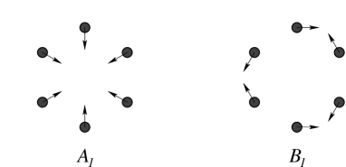
Figure 2: Phonon modes responsible for the $D^{*}$ Raman peak.

We restrict our attention to scalar phonons with wave vectors close to $K$ and $K^{\prime}$ points – those responsible for the $D^{*}$ Raman peak. The two real linear combinations of the modes at $K$ and $K^{\prime}$ points transform according to $A_{1}$ and $B_{1}$ representations of $C_{6v}$ and are shown in Fig. 2. We take the magnitude of the carbon atom displacement as the normal coordinate for each mode, denoted by $u_{a}$ and $u_{b}$, respectively. Upon quantization of the phonon field, $\hat{u}_{a},\hat{u}_{b}$ and the phonon hamiltonian $\hat{H}_{\mathrm{ph}}$ are expressed in terms of the creation and annihilation operators $\hat{b}^{\dagger}_{{\rm\bf q}\mu},\hat{b}_{{\rm\bf q}\mu}$, $\mu=a,b$, as

$$\hat{u}_{\mu}({\rm\bf r})=\sum_{{\rm\bf q}}\frac{\hat{b}_{{\rm\bf q}\mu}e^{i{\rm\bf q}{\rm\bf r}}+\mathrm{h.c.}}{\sqrt{2NM\omega_{A_{1}}}},\quad\hat{H}_{\mathrm{ph}}=\sum_{{\rm\bf q},\mu}\omega_{A_{1}}\hat{b}_{{\rm\bf q}\mu}^{\dagger}\hat{b}_{{\rm\bf q}\mu}.$$ (3)

The crystal is assumed to have the area $L_{x}L_{y}$, and to contain $N$ carbon atoms of mass $M$. The ${\rm\bf q}$ summation is performed as $\sum_{\rm\bf q}\to{L}_{x}L_{y}\int{d}^{2}{\rm\bf q}/(2\pi)^{2}$. “h.c.” stands for hermitian conjugate. By symmetry, in the electron-phonon interaction hamiltonian Heph the normal displacements $u_{\mu}$ couple to the corresponding valley-off-diagonal $4\times{4}$ matrices from Table 2:

$$\hat{H}_{int}=3F_{A_{1}}\int{d}^{2}{\rm\bf r}\,\hat{\psi}^{\dagger}({\rm\bf r})\left[\hat{u}_{a}({\rm\bf r})\Lambda_{x}\Sigma_{z}+\hat{u}_{b}({\rm\bf r})\Lambda_{y}\Sigma_{z}\right]\hat{\psi}({\rm\bf r}).$$ (4)

Interaction with light is obtained from the Dirac hamiltonian (2) by replacement ${\rm\bf\nabla}\to{\rm\bf\nabla}-i(e/c)\hat{{\rm\bf A}}$, where the vector potential $\hat{{\rm\bf A}}$ is expressed in terms of creation and annihilation operators $\hat{a}^{\dagger}_{{\rm\bf Q},\ell},\hat{a}_{{\rm\bf Q},\ell}$ of three-dimensional photons in the quantization volume $V=L_{x}L_{y}L_{z}$, labeled by the wave vector ${\rm\bf Q}$ and two transverse polarizations $\ell=1,2$ with unit vectors ${\rm\bf e}_{{\rm\bf Q},\ell}$:

$$\hat{{\rm\bf A}}({\rm\bf r})=\sum_{{\rm\bf Q},\ell}\sqrt{\frac{2\pi{c}}{VQ}}\left({\rm\bf e}_{{\rm\bf Q},\ell}\hat{a}_{{\rm\bf Q},\ell}e^{i{\rm\bf Q}{\rm\bf r}}+\mathrm{h.c.}\right).$$ (5)

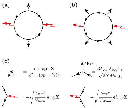
Figure 3: (a), (b) Fully resonant diagrams giving the matrix element $\mathcal{M}$ for the two- and four-phonon Raman scattering, respectively. Other possible diagrams (not shown) are not fully resonant, and are smaller by a factor $\sim\gamma/\omega_{A_{1}}$. (c) Analytical expressions, corresponding to lines and vertices of the diagrams. In the electron loop integration over the internal momentum and energy, as well as tracing over $4\times{4}$ matrix structure should be performed.

Calculation.— $\mathcal{M}({\rm\bf q}_{1},\mu_{1};\ldots;{\rm\bf q}_{n},\mu_{n})$, the matrix element of the transition from the state with one incoming photon (frequency $\omega_{in}$, polarization ${\rm\bf e}_{in}$) into the state with one outgoing photon (frequency $\omega_{out}$, polarization ${\rm\bf e}_{out}$) and $n$ phonons (modes $\mu_{1},\ldots,\mu_{n}$, wave vectors ${\rm\bf q}_{1},\ldots,{\rm\bf q}_{n}$), is calculated as shown in Fig. 3. We emphasize the necessity to include the inelastic broadening $\gamma$ in the electronic Green’s functions, as the dominant contribution to the integral comes from regions where the denominators are small ($\sim\gamma$, corresponding to real electrons and holes, as discussed above). Given the matrix element, we sum over final photon and phonon states, and express the absolute dimensionless probability of $n$-phonon Raman scattering as

$$I_{n} = \frac{V^{2}}{c^{2}}\,\frac{L_{x}L_{y}\omega_{out}^{2}}{2\pi^{2}{c}^{2}}\frac{1}{n!}\times$$ (6)

$$\times\sum_{{\rm\bf q}_{1}+\ldots+{\rm\bf q}_{n}=0}\sum_{\{\mu_{i}\}}\left|\sum_{\mathcal{P}}\mathcal{M}\!\left({\mathcal{P}\{{\rm\bf q}_{i},\mu_{i}\}}\right)\right|^{2},$$

where $\mathcal{P}$ denotes permutations of phonon arguments.

For the $D^{*}$ peak the diagram in Fig. 3a gives

$$\mathcal{M}({\rm\bf q})=\frac{\pi{e}^{2}/V}{\sqrt{\omega_{in}+\omega_{out}}}\,\frac{9F_{A_{1}}^{2}/4}{NM\omega_{A_{1}}}\,\frac{[{\rm\bf e}_{{\rm\bf q}}\times{\rm\bf e}_{in}]_{z}[{\rm\bf e}_{{\rm\bf q}}\times{\rm\bf e}_{out}^{*}]_{z}}{[v(q-q_{bs})-2i\gamma]^{3/2}},$$ (7)

where ${\rm\bf e}_{{\rm\bf q}}\equiv{\rm\bf q}/|{\rm\bf q}|$. The value $q_{bs}=(\omega_{in}+\omega_{out})/(2v)$, around which expression (7) is strongly peaked, corresponds to backscattering of the electron and the hole by the phonons. This sharply peaked dependence cannot be obtained from pure symmetry considerations, which just prescribe vanishing of the matrix element when the scattering angle $\varphi=0$ Maultzsch . Its origin is the quasiclassical nature of the electron and hole motion thickpaper , the dispersion of $\varphi$ being determined by quantum diffraction: $|\varphi-\pi|\sim\sqrt{\gamma/\omega_{in}}\ll{1}$. One consequence of this peaked dependence is that the width of the $D^{*}$ peak is determined by the electron and phonon lifetimes only, not by the phonon dispersion. Besides, it should lead to a significant polarization anisotropy of the $D^{*}$ peak thickpaper . Here we simply sum over the polarizations; substituting Eq. (7) into Eq. (6) and approximating $\omega_{out}\approx\omega_{in}$, we obtain:

$$I_{D^{*}}=\frac{(e^{2}/c)^{2}}{48\pi}\frac{v^{2}}{c^{2}}\frac{\omega_{in}^{2}}{\gamma^{2}}\left[\frac{9F_{A_{1}}^{2}}{M\omega_{A_{1}}v^{2}}\frac{\sqrt{27}a^{2}}{4}\right]^{2}.$$ (8)

We can allow for trigonal warping and electron-hole asymmetry terms in the dispersion of electrons and holes: $\pm{v}p\to\pm(vp+\alpha_{3}p^{2}\cos{3}\varphi_{{\rm\bf p}})+\alpha_{0}p^{2}$, where $\varphi_{{\rm\bf p}}$ is the polar angle of ${\rm\bf p}$, tight-binding model gives $\alpha_{3}=va/4$ ($v\approx{10}^{8}\>\mathrm{cm/s}$, $a\approx{1}.42\>\mbox{\AA}$), and $\alpha_{0}(1\>\mbox{eV})^{2}/v^{2}\sim{0}.1\>\mbox{eV}$ DresselhausBook . The relative corrections to expression (8) from these terms are $(9/8)(\alpha_{3}\omega_{A_{1}}/v^{2})^{2}\sim{10}^{-4}$ and $-[\alpha_{0}(\omega_{in}\omega_{A_{1}}/v^{2})/(2\gamma)]^{2}/2\sim{10}^{-4}(\omega_{in}/2\gamma)^{2}$.

Evaluation of the diagram in Fig. 3b gives the intensity of the four-phonon Raman peak:

$$I_{2D^{*}}=0.088\,\frac{(e^{2}/c)^{2}}{64\pi^{4}}\frac{v^{2}}{c^{2}}\frac{\omega_{in}^{4}}{\gamma^{4}}\left[\frac{9F_{A_{1}}^{2}}{M\omega_{A_{1}}v^{2}}\frac{\sqrt{27}a^{2}}{4}\right]^{4}.$$ (9)

Figure 4: The self-energy diagram describing the phonon emission. The dashed line represents the phonon Green’s function $D({\rm\bf q},\omega)=2\omega_{A_{1}}/[\omega^{2}-(\omega_{A_{1}}-io)^{2}]$.

Finally, we express the Raman scattering probabilities in terms of the phonon emission rate. The latter is given by the imaginary part of the self-energy (Fig. 4):

$$\gamma_{A_{1}}(\epsilon)=\frac{9F^{2}_{A_{1}}}{M\omega_{A_{1}}v^{2}}\frac{\sqrt{27}a^{2}}{4}\,\frac{|\epsilon|-\omega_{A_{1}}}{4}\,\theta(|\epsilon|-\omega_{A_{1}}),$$ (10)

where $\theta(\epsilon)$ is a step function. Eqs. (8), (9) and Eq. (10) with $\epsilon=\omega_{in}/2$ give Eq. (1).

Instead of conclusion, we quote an experimental value for the ratio $I_{D^{*}}/I_{2D^{*}}\approx{40}$ expdata , so Eq. (1) gives $\gamma_{A_{1}}/\gamma\approx{0}.42$. We assume $\gamma=\gamma_{A_{1}}+\gamma_{E_{2}}+\gamma_{ee}$ and note that the emission rate $2\gamma_{E_{2}}$ of $E_{2}$ phonons is described by Eq. (10), with the replacements $F_{A_{1}}\to{F}_{E_{2}}$ (the corresponding coupling constant), $\omega_{A_{1}}\to\omega_{E_{2}}$. In the tight-binding model $F_{A_{1}}=F_{E_{2}}$ (for the normalization of the phonon displacements chosen here), which agrees with a DFT calculation Piscanec up to 1%. The assumption $F_{A_{1}}=F_{E_{2}}$ gives $\gamma_{ee}\approx{0}.22\,\gamma$.

On the other hand, $F_{A_{1}}$ and $F_{E_{2}}$ are not related by any symmetry. For intensities of the two-phonon Raman peaks $D^{*}$ and $G^{*}$ our calculation gives $I_{D^{*}}/I_{G^{*}}=2(F_{A_{1}}/F_{E_{2}})^{4}(\omega_{E_{2}}/\omega_{A_{1}})^{2}$, the experimental value being $I_{D^{*}}/I_{G^{*}}\approx{20}$ Ferrari ; expdata . This suggests $F_{A_{1}}/F_{E_{2}}\approx{1}.6$, in significant disagreement with the tight-binding model prescription. Substituted in Eq. (1), it gives $\gamma_{ee}\approx{0}.44\,\gamma$, which agrees with the calculated $2\gamma_{ee}\approx{10}$ meV Rubio and the total $2\gamma$ measured by time-resolved photoemission spectroscopy (20 meV in Ref. Gao , $25$ meV in Ref. Moos , all values taken for $\epsilon=\omega_{in}/2=1$ eV). Even though a recent ARPES measurement gives a significantly larger value for $2\gamma\sim{100}\>\mbox{meV}$ Rotenberg , the issue of validity of the tight-binding model for electron-phonon coupling seems to deserve further investigation.

The author thanks I. L. Aleiner and J. Yan for stimulating discussions and critical reading of the manuscript, and Y. Wu for sharing unpublished experimental results.

References

- (1) J. González, F. Guinea, and M. A. H. Vozmediano, Phys. Rev. Lett. 77, 3589 (1996).
- (2) C. D. Spataru et al., Phys. Rev. Lett. 87, 246405 (2001).
- (3) E. H. Hwang, B. Y.-K. Hu, and S. Das Sarma, cond-mat/0612345.
- (4) A. C. Ferrari et al., Phys. Rev. Lett. 97, 187401 (2006).
- (5) A. Gupta et al., cond-mat/0606593.
- (6) D. Graf et al., Nano Lett. 7, 238 (2007).
- (7) S. Pisana et al., Nature Materials 6, 198 (2007).
- (8) J. Yan et al., Phys. Rev. Lett. 98 166802 (2007).
- (9) M. Lazzeri and F. Mauri, Phys. Rev. Lett. 97, 266407 (2006).
- (10) A. H. Castro Neto and F. Guinea, Phys. Rev. B 75, 045404 (2007).
- (11) C. Thomsen and S. Reich, Phys. Rev. Lett. 85, 5214 (2000).
- (12) R. C. C. Leite, J. F. Scott, and T. C. Damen, Phys. Rev. Lett. 22, 780 (1969).
- (13) M. V. Klein and S. P. S. Porto, Phys. Rev. Lett. 22, 782 (1969).
- (14) R. M. Martin and C. M. Varma, Phys. Rev. Lett. 26, 1241 (1971).
- (15) R. Zeyher, Solid State Commun. 16, 49 (1975).
- (16) E. McCann et al., Phys. Rev. Lett. 97, 146805 (2006).
- (17) I. L. Aleiner and K. B. Efetov, Phys. Rev. Lett. 97, 236801 (2006).
- (18) Hamiltonian (4) can be derived microscopically, e. g., in the tight-binding model. Then , where is the nearest-neighbor coupling matrix element, and is the bond length. Our calculation, however, does not rely on the tight-binding approximation.
- (19) J. Maultzsch, S. Reich, and C. Thomsen, Phys. Rev. B 70, 155403 (2004).
- (20) D. M. Basko and I. L. Aleiner, to be published.
- (21) R. Saito, G. Dresselhaus, and M. S. Dresselhaus, Physical Properties of Carbon Nanotubes (Imperial College Press, London, 1998).
- (22) Y. Wu (unpublished); in this measurement eV.
- (23) S. Piscanec et al., Phys. Rev. Lett. 93, 185503 (2004).
- (24) S. Xu et al., Phys. Rev. Lett. 76, 483 (1996).
- (25) G. Moos et al., Phys. Rev. Lett. 87, 267402 (2001).
- (26) A. Bostwick et al., Nature Physics 3, 36 (2007).