Lifetime of Stringy de Sitter Vacua

Abstract:

In this note we perform a synopsis of the life-times from vacuum decay of several de Sitter vacuum constructions in string/M-theory which have a single dS minimum arising from lifting a pre-existing AdS extremum and no other local minima existent after lifting. For these vacua the decay proceeds via a Coleman–De Luccia instanton towards the universal Minkowski minimum at infinite volume. This can be calculated using the thin–wall approximation, provided the cosmological constant of the local dS minimum is tuned sufficiently small. We compare the estimates for the different model classes and find them all stable in the sense of exponentially long life times as long as they have a very small cosmological constant and a scale of supersymmetry breaking $\lower 3.01385pt\hbox{$\;\stackrel{{\scriptstyle\textstyle>}}{{\sim}}\;$}{\rm TeV}$.

1 Introduction

The ongoing search for de Sitter (dS) vacua in string theory - motivated in part by the recent cosmological data pointing towards a tiny non-vanishing positive cosmological constant $\Lambda$ - has so far produced semi-explicit examples firstly [1] in the context of flux compactification of the type IIB superstring along the lines of [2] and, recently, also in the context of M-theory compactified on 7-dimensional manifolds of $G_{2}$-holonomy without fluxes [3, 4, 5] and strongly coupled heterotic M-theory with fluxes on $CY_{3}\times S^{1}/Z_{2}$ [6, 7].

The first three examples have in common that the type IIB axio-dilaton $S$ and the complex structure moduli $U$ of the 6d compact Calabi-Yau 3-fold are fixed by quantized p-form background fluxes. These fluxes induce a superpotential for the complex structure moduli and the dilaton of the Gukov-Wafa-Witten type [8].

The fourth example in M-theory does not use fluxes but instead uses a racetrack superpotential generated by non-perturbative effects like membrane instantons or gaugino condensation to stabilize all M-theory moduli in one step [9, 10].

The fifth example consists of strongly coupled heterotic M-theory with fluxes compactified on $CY_{3}\times S^{1}/Z_{2}$ [6, 7]. Here, again fluxes stabilize the non-universal moduli, while the Calabi-Yau volume, the orbifold length and the dilaton are stabilized by non-perturbative effects from gaugino condensation, $M2$- and $M5$-brane instantons.

The first class of models - initiated by KKLT [1] - stabilizes the complex structure moduli and the dilaton with background fluxes. Then they fix the remaining Kähler moduli with non-perturbative effects like gaugino condensation on $D7$-branes wrapping 4-cycles of the Calabi-Yau or 4-cycle wrapping Euclidean $D3$-brane instantons. This produces SUSY anti de Sitter (AdS) vacua for all the moduli. The uplifting to dS vacua then proceeds:

• by either introducing an explicitly SUSY breaking $\overline{D3}$-brane [1],

• by supersymmetric D-terms from magnetic world volume fluxes of 4-cycle wrapping $D7$-branes [11, 12, 13, 14, 15],

• by the backreaction of $D3$-branes which can provide for a supersymmetric uplifting of a form similar to that of the KKLT $\overline{D3}$-brane [16]

• by supersymmetric F-terms from the F-terms of hidden sector matter fields [17] (see also [18]) or uplifting in (F-term induced) metastable vacua [19, 20, 21, 22] along the lines of the ISS-model of SUSY breaking in meta-stable vacua [23]

• or without additional extended sources by taking into account the effect of the leading higher-order ${\cal O}(\alpha^{\prime 3})$-correction [24] into the process of stabilizing the Kähler moduli with non-perturbative effects [25, 26, 27].

This class of models is characterized by a fine tuning of the flux superpotential towards small negative values in order to realize vacua at volumes of ${\cal O}(100)$. The common feature of all the constructions in this class is that the non-perturbative terms in the superpotential determine a lower bound on the width of potential barrier which separates their dS minima from a Minkowski minimum at infinite volume. This is due to the fact that the non-perturbative effects fall off with increasing volume faster than any of the uplifts which have inverse power-law dependence on the volume.

In the second class of models by Balasubramanian, Berglund, Conlon and Quevedo - the ’large volume scenario’ (LVS) [28, 29] the stabilization of the Kähler moduli proceeds via the combined effects of the leading $\alpha^{\prime}$-correction [24] with the non-perturbative effects which produces non-SUSY AdS vacua at exponentially large volumes - thus the name. Uplifting then proceeds either via $\overline{D3}$-branes or D-terms. These models do not need to have $W_{\rm flux}$ to be tuned small.

The third class of models differs in that the stabilization of the Kähler moduli proceeds solely through the inclusion of perturbative contributions to the moduli potential. No non-perturbative effects are needed or included. This was done first by compactifying type IIB string theory on Riemann surfaces with closed string fluxes in the presence of $D7$-branes [30] (see also [31] for related earlier work in non-critical string theory). This gives, using the fluxes and branes, enough perturbative contributions to the moduli potential to stabilize the complex structure moduli, the dilaton and the Kähler moduli altogether in de Sitter vacua. Then, in type IIB flux compactifications along [2], where closed string fluxes fix the complex structures and the dilaton, the stabilization of the volume can proceed through the inclusion of perturbative corrections of higher order in $\alpha^{\prime}$ and the string coupling $g_{S}$ to the tree level Kähler potential: Besides the leading $\alpha^{\prime}$-correction [24] there exists a string 1-loop correction [33] to $K$ which together manage to stabilize the volume Kähler modulus upon a certain tuning of the flux superpotential at moderately large values in a non-SUSY AdS vacuum [34, 35]. Since SUSY is broken in these vacua and the perturbative nature of the stabilization respects certain shift symmetries of the underlying string theory, a gauging of these symmetries via magnetic world volume flux on a 4-cycle wrapping $D7$-brane then provides an explicit way to uplift these minima to become dS vacua [36]. Note, that for the above two examples in this class the resulting moduli potential for the Kähler moduli is qualitatively similar in that it consists of several terms of the form $g_{S}^{r}/{\cal V}^{s}$ ($s\geq 2$) with different signs which thus compete to stabilize the volume ${\cal V}$. Therefore, we will proceed later on to analyze the life-time calculation in the semi-explicit toroidal orientifold example of Kähler stabilized dS vacua of [34, 35, 36], with the notion in mind that the parametrical life-time estimate obtained there will carry over to the example in [30] of type IIB on Riemann surfaces for the above reason.

The fourth class differs significantly in that M-theory compactified on $G_{2}$-manifolds does not use any background flux. Non-perturbative effects generating a racetrack superpotential are used alone to stabilize all the M-theory moduli while the F-terms of hidden sector charged matter terms allow for a positive vacuum energy. The critical ingredient here is that in M-theory the non-perturbative superpotential generically depends on all moduli [9, 10]. This is different from both the situation of the weakly coupled heterotic string (where racetrack construction to stabilize the dilaton are well studied in the literature) as well as of type IIB string theory where the non-perturbative effects generically depend on the Kähler but not on the complex structure moduli.

Finally, the fifth class of models in strongly coupled heterotic M-theory on $CY_{3}\times S^{1}/Z_{2}$ [6, 7] is in part similar to the KKLT like constructions in that all the non-universal moduli get string scale masses as they are fixed by background flux. The remaining universal moduli, consisting of the dilaton, the $CY_{3}$-volume and the orbifold length, are then stabilized by a combination of non-perturbative effects alone [7] which resembles the situation in [9, 10]. The results we get explicitly for the $G_{2}$-model of [9, 10] will thus carry over to the construction of [7] because the decay there also proceeds in the decompactificying runaway directions of the universal moduli.

All constructions have in common that they produce a dS vacuum at tiny positive values $V_{0}$ of the vacuum energy which is separated by a high potential barrier $V_{1}\gg V_{0}$ from a Minkowski minimum at infinite volume which corresponds to spontaneous decompactification of the compact dimensions. These dS vacua therefore are just metastable under formation of the lower-energy Minkowski vacuum by quantum mechanical tunneling. This process is described by the Coleman-De-Luccia (CDL) instanton [37]. In this note we shall then review (for some examples) and calculate (for the other examples) the life–time of the dS vacuum and show that they are all exponentially long–lived.

2 Metastability of a dS vacuum

We shall start the discussion thus with summarizing the results of [37] which according to [1] go as follows. If the potential energy difference $\Delta V=V_{0}-V_{\infty}$ of two vacua participating in the tunneling event is small compared to height of barrier $V_{1}$ separating them, i.e.

$$V_{1}\gg|\Delta V|\;\;,$$ (1)

then the thin-wall approximation becomes applicable. Within this approximation we get the tunneling rate as

$$\Gamma\sim e^{-\frac{S_{\rm E}(\phi_{0})}{(1+4\Delta V/3T^{2})^{2}}}$$ (2)

where $T$ denotes the tension of wall of the nucleated bubbles of new vacuum

$$T=\int_{\phi_{0}}^{\phi_{\infty}}d\phi\,\sqrt{2\,V(\phi)}\;.$$ (3)

Here $S_{\rm E}$ denotes the Euclidean action of the scalar field $\phi$ evaluated at the initial vacuum $\phi_{0}$. Further, $\phi$ denotes the canonically normalized direction in scalar field space along which the tunneling proceeds - i.e. the one with lowest and thinnest potential barrier. If, as in our cases here, the initial vacuum is de Sitter with vacuum energy $V_{0}$ and the final vacuum is Minkowski, then the expression for the CDL instanton becomes

$$\Gamma\sim e^{-\frac{S_{\rm E}(\phi_{0})}{(1+4V_{0}/3T^{2})^{2}}}\;.$$ (4)

Approximating the bubble wall tension with

$$T\sim\sqrt{V_{1}}\,\Delta\phi$$ (5)

with $\Delta\phi$ denoting the potential barrier thickness, one arrives at a universal expression for the decay rate

$$\Gamma\sim e^{-S_{\rm E}(\phi_{0})}=e^{-\frac{24\pi^{2}}{V_{0}}}$$ (6)

as long as [1, 37]

$$V_{0}\ll T^{2}\;\Leftrightarrow(\Delta\phi)^{2}\gg\frac{V_{0}}{V_{1}}\;.$$ (7)

Since $V_{0}\ll V_{1}$ holds in all the three classes of dS constructions discussed above it remains to check that the barrier thickness is not too small (in the above sense): i.e. $\Delta\phi={\cal O}(0.1\ldots 1)$ would guarantee the longevity of the dS vacua in all constructions as long as $V_{1}\gg V_{0}$ and $V_{0}\sim 10^{-120}$. Since

$$V_{1}\sim-V_{\rm AdS\;min.}\sim\left.\frac{|W|^{2}}{(T+\bar{T})^{n}}\right|_{T=T_{\rm dS\;min.}}\;,\;3\leq n<5$$ (8)

in all three model classes $V_{1}\gg V_{0}$ will hold for not too small values of $W$ and the compact volume ${\cal V}=(T+\bar{T})^{3/2}$ for all of them.

Thus, it remains to check $\Delta\phi={\cal O}(10^{-3}\ldots 1)$ to establish the longevity of the dS vacua in all constructions. While this has been done for the KKLT-like constructions [1], which will be recapped in Section 4.1, to the knowledge of the author this has not been done for the LVS model [29] and the Kähler stabilization based dS construction [36]. The following will summarize how to determine the barrier thickness $\Delta\phi$ in these latter constructions. The upshot will be that after identifying the proper canonically normalized field $\phi$ in terms of the Kähler modulus $T$ in each type of construction we will find $\Delta\phi={\cal O}(10^{-3}\ldots 1)$ to be valid. This will then establish the longevity of their dS vacua.

Let us note here that the above estimates hold only for the case that the scalar potential contains just a single dS minimum that has as its final state after the decay only the decompactifying Minkowski vacuum at infinite volume. This can be different if the structure of the scalar potential prior to uplifting is more complicated. Consider as an example a dS vacuum arising from, say, a scalar potential which has two AdS minima of different depth prior to uplifting, where the more shallow AdS minimum shall be at smaller volume. Assume further that SUSY breaking would lift the more shallow AdS minimum to become the fine-tuned small-$\Lambda$ dS minimum as, e.g., in the Kallosh-Linde model [38]. Then the decay rate would be enhanced by tens of orders of magnitude compared to the estimate (6) as shown in [39].

Thus we shall constrain ourselves here to the study of the simple cases where the dS minimum arises from the uplifting of a scalar potential with a single AdS minimum. This yields afterwards just the dS vacuum and a barrier separating the local minimum from the Minkowski vacuum at infinite volume.

3 Estimating the barrier width $\Delta\phi$

Let us now outline the method of how to determine the barrier width $\Delta\phi$ parametrically. In all three classes of models the 4d ${\cal N}=1$ supergravity AdS scalar potential prior to uplifting depends on an inverse power of the volume which is larger than that of the positive semi-definite uplifting potentials

$$V_{\rm AdS}=e^{K}(K^{T_{j}\bar{T}_{k}}D_{T_{j}}W\overline{D_{T_{k}}W}-3|W|^{2})\sim\left\{\begin{array}[]{c}e^{-a_{j}\cdot T_{j}}/{\cal V}^{2}\;,\;\textrm{KKLT}\\ 1/{\cal V}^{n}\;,\;n\geq 3\;\;\textrm{else}\end{array}\right.$$ (9)

while

$$V_{\rm uplift}\sim\frac{1}{{\cal V}^{s}}\;,\;s\leq 2\;.$$ (10)

Thus, after uplifting the part of the potential barrier residing at values ${\rm Re}\,T>{\rm Re}\,T_{1}$ will be wider than the other part of the barrier situated between the dS minimum $V_{0}$ at $T_{0}$ and the barrier maximum $V_{1}$ at $T_{1}$.

For instance, in the KKLT construction (assuming just one Kähler modulus for simplicity) we have

$$K = -3\ln(T+\bar{T})\;\;,\;T=t+i\,b$$

$$W = W_{0}+A\,e^{-a\cdot T}\;,\;W_{0}=W_{\rm flux}$$

combined with an uplift from an $\overline{D3}$-brane which yields

$$V(T)=e^{K}(K^{T\bar{T}}D_{T}W\overline{D_{T}W}-3|W|^{2})+\frac{D}{({\rm Re}\,T)^{2}}\;\;.$$ (12)

Here $b$ denotes the 4d scalar axion partner of the 4-cycle volume measured by $t$.

Fig. 1 shows the situation which exemplifies the asymmetric distribution of the barrier width around the barrier maximum described above.

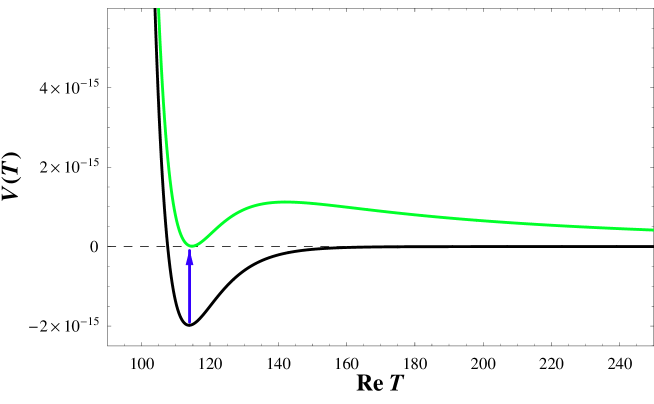
Figure 1: Black: The F-term scalar potential $V_{F}(T)$ leading to the stabilization of $T$. Green: The scalar potential eq. (12) after uplifting by switching on a single $\overline{D3}$-brane.

In view of this asymmetric barrier width, a conservative estimate of the width should be given by taking

$$\Delta{\rm Re}\,T\sim 2\cdot({\rm Re}\,T_{1}-{\rm Re}\,T_{0})$$ (13)

where as before $T_{0}$ denotes the position of the dS minimum and $T_{1}$ the one of the barrier maximum. Further, an estimate of ${\rm Re}\,T_{1}$ follows from the fact, that the barrier maximum arises at that point where the AdS scalar potential prior to uplifting has decreased its magnitude significantly compared to its value at the AdS minimum when going towards larger ${\rm Re}\,T$. We can thus take

$${\rm Re}\,T_{1}:\;|V_{\rm AdS}(T_{1})|=\epsilon\cdot|V_{\rm AdS}(T_{0})|\;{\rm with}\;\epsilon={\cal O}(0.1)\;{\rm and}\;{\rm Re}\,T_{1}>{\rm Re}\,T_{0}\;\;.$$ (14)

Using this in eq. (13) should then provide us with a conservative parametrical estimate of the barrier width in terms of the field $T$. Next, note that the field $T$ is not canonically normalized. However, a look at its Kähler potential $K=-3\ln(T+\bar{T})$ allows as to define the canonically normalized field we need for calculating the barrier width used in eq.s (4), (5) as [1]

$$\phi=\sqrt{\frac{3}{2}}\cdot\ln({\rm Re}\,T)\;.$$ (15)

From here we arrive finally at a parametrical expression for the barrier width $\Delta\phi$ given by

$$\Delta\phi\sim\sqrt{6}\cdot\ln\left(\frac{{\rm Re}\,T_{1}}{{\rm Re}\,T_{0}}\right)\;\;.$$ (16)

In the following Chapter we will apply this formalism to the three classes of models discussed above.

4 Comparing the existing constructions

4.1 KKLT-like dS constructions

The KKLT construction is described in 4d by the ${\cal N}=1$ chiral ungauged supergravity specified by the Kähler potential and superpotential of eq. (LABEL:KWkklt). According to the method outlined in the last Section we determine the barrier width of the positive semi-definite scalar potential after uplifting by extracting the position $T_{0}$ of the AdS vacuum prior to uplifting (which is close to the position of the later dS minimum) and the position $T_{1}$ of the barrier maximum. The former is given by the solution to

$$\left.D_{T}W\right|_{T_{0}}=-aA\,e^{-aT_{0}}-\frac{3\,(W_{0}+A\,e^{-aT_{0}})}{T_{0}+\bar{T}_{0}}=0\;.$$ (17)

Now from here we can infer the position $T_{1}$ of barrier maximum directly: At $T_{1}=T_{0}+1/a$ the exponential contribution in $W$ is down by a factor of $1/e$ which implies that

$$\left.D_{T}W\right|_{T_{1}=T_{0}+1/a}\approx-\frac{3\,W_{0}}{T_{1}+\bar{T}_{1}}\;.$$ (18)

However, this expression is the no-scale result which implies that at this value of $T_{1}$ we have $K^{T\bar{T}}D_{T}W\overline{D_{T}W}\approx 3|W|^{2}$ and thus $V_{\rm AdS}(T_{1})\approx 0$. Using eq. (16) this gives us the barrier width in terms of canonically normalized field $\phi$ as

$$\Delta\phi_{\rm KKLT}\sim\sqrt{6}\cdot\ln\left(\frac{t_{0}+1/a}{t_{0}}\right)=\frac{\sqrt{6}}{a\,t_{0}}+{\cal O}\left(\frac{1}{(a\,t_{0})^{2}}\right)\;.$$ (19)

Validity of the supergravity approximation requires $t_{0}\gg 1$ and $a\,t_{0}\gg 1$ - typical model constructions have $t_{0}={\cal O}(100)$ and $a\,t_{0}={\cal O}(10)$. Thus, in KKLT–like models we have typically

$$(\Delta\phi_{\rm KKLT})^{2}=0.01\ldots 0.1\gg\frac{V_{0}}{V_{1}}$$ (20)

in accordance with the requirement of eq. (7). This in turn implies that the lifetime of the dS vacuum is given from eq. (6) as [1]

$$\tau_{\rm KKLT}\sim\Gamma_{\rm KKLT}^{-1}\sim e^{\frac{24\pi^{2}}{V_{0}}}\,t_{P}\sim e^{10^{120}}\,t_{P}\;\;{\rm for}\;V_{0}\sim 10^{-120}$$ (21)

where $t_{P}\sim 10^{-43}\,s$ denotes the Planck time. Note that these estimates apply directly also to all the other KKLT-like de Sitter vacua constructions in this first class of models (see Section 1.1) along the lines of [11, 12, 13, 14, 16, 19, 20, 21, 22, 18, 25, 26, 27]. This derives from the fact that in all constructions their respective F–term or D–term uplifting produces a $\delta V_{\rm uplift}=C/(T+\bar{T})^{n}$ which imitates the effect of the $\overline{D3}$-brane of KKLT.

4.2 LVS type large-volume dS constructions

This class of models [28] is based on a compactification of the type IIB superstring on the orientifolded $\mathbb{P}_{[1,1,1,6,9]}^{4}$ del Pezzo surface. This manifold has $h^{1,1}=2$ Kähler moduli and $h^{2,1}=272$ complex structure moduli which latter ones can be stabilized by turning on the closed string background fluxes. The remaining two Kähler moduli, called $T_{4}$ and ₅ in what follows, are then fixed by introducing non-perturbative superpotential contributions coupling to each of them and the inclusion of leading $\alpha^{\prime}$-correction to the Kähler potential. The model is then described in 4d by a Kähler potential and a superpotential as follows

$$K = -2\ln{\cal V}-\frac{C_{\alpha^{\prime}}}{\cal V}+\ldots\;,\;{\cal V}=\frac{1}{9\sqrt{2}}\,(t_{5}^{3/2}-t_{4}^{3/2})$$

$$W = W_{0}+A_{4}\,e^{-a_{4}\cdot T_{4}}+A_{5}\,e^{-a_{5}\cdot T_{5}}$$

The constant $C_{\alpha^{\prime}}$ can be computed in this model and is given by [24, 28, 29]

$$C_{\alpha^{\prime}}=\underbrace{-\frac{1}{2}\,\zeta(3)\chi}_{\xi}\cdot({\rm Re}\,S)^{3/2}\;\;{\rm with:}\;\chi=2\,(h^{1,1}-h^{2,1})=-540\;.$$ (23)

The corresponding F-term scalar potential $V_{\rm AdS}$ from eq. (9) takes in the region where $t_{5}\gg t_{4}>1$ the approximate form

$$V_{\rm AdS}=\frac{|W_{0}|^{2}}{{\cal V}^{3}}\,(-\mu\ln{\cal V}+\lambda\sqrt{\ln{\cal V}}+\nu\,\xi)\;\;.$$ (24)

This potential fixes the Kähler moduli in a SUSY breaking AdS minimum at $(t_{5,0},t_{4,0})$ such that $t_{5,0}\gg t_{4,0}>1$ [28, 29]. Because of this regime we have ${\cal V}=t_{5}^{3/2}/9\sqrt{2}$ to a very good accuracy at this AdS minimum implying that tunneling to the decompactifying Minkowski minimum at infinity will occur practically completely in the $t_{5}$-direction in scalar field space. The potential approaches zero from below beyond the AdS minimum and thus can be approximated there as

$$V_{\rm AdS}\sim-\,|W_{0}|^{2}\cdot\frac{\mu\ln{\cal V}}{{\cal V}^{3}}\sim-\,\frac{\mu\,|W_{0}|^{2}}{972\sqrt{2}}\cdot\frac{\ln t_{5}}{t_{5}^{9/2}}\;\;{\rm for}\;t_{5}>t_{5,0}\;.$$ (25)

Now we can apply eq. (14) to extract $t_{5,1}$, i.e. the position where $|V_{\rm AdS}(T_{5,1})|\ll|V_{\rm AdS}(T_{5,0})|$, as

$$t_{5,1}=t_{5,0}\cdot\left[1+\frac{2}{9}\gamma+{\cal O}(\gamma^{2})\right]\;\;{\rm where}\;\gamma=1-\epsilon\;\;.$$ (26)

This allows us to compute the barrier width which the dS vacuum resulting from uplifting the above AdS minimum with, e.g., a D-term will have in terms of the canonically normalized ’tunneling’ field $\phi$ from eq. (16) to yield

$$\Delta\phi_{\rm LVS} \sim \sqrt{6}\cdot\ln\left(\frac{t_{5,1}}{t_{5,0}}\right)\sim\left(\frac{2}{3}\right)^{3/2}\cdot(1-\epsilon)=0.05\ldots 0.2\;\;{\rm for}\;\epsilon=0.1\ldots 0.2$$ (27)

$$\;\Rightarrow(\Delta\phi_{\rm LVS})^{2}\sim 10^{-3}\ldots 10^{-2}\gg\frac{V_{0}}{V_{1}}$$

This result is parametrically similar to the KKLT-like models and thus a similar estimate results for lifetime of the dS vacua in these large-volume vacua

$$\tau_{\rm LVS}\sim\Gamma_{\rm LVS}^{-1}\sim e^{\frac{24\pi^{2}}{V_{0}}}\,t_{P}\sim e^{10^{120}}\,t_{P}\;\;{\rm for}\;V_{0}\sim 10^{-120}\;\;.$$ (28)

We note finally, that these results are stable under the addition of further string loop corrections, as the whole LVS construction has recently been shown to be stable when taking into account these corrections [40].

4.3 D-term uplifted Kähler stabilization dS construction

This example of the third class of models arises from the observation that the combined effects of the leading perturbative $\alpha^{\prime}$-correction and 1-loop correction to the Kähler potential suffice in presence of the flux superpotential to stabilize the volume Kähler modulus [34]. No non-perturbative effects are needed here.

Notice, that that the ensuing discussion will carry over qualitatively to the other example in this class [30] (type IIB on Riemann surfaces). This is due to the fact that the resulting moduli potential for the Kähler moduli is qualitatively similar for both examples in that it consists of several terms of the form $g_{S}^{r}/{\cal V}^{s}$ ($s\geq 2$) with different signs which thus compete to stabilize the volume ${\cal V}$. Therefore, we choose to analyze the life-time calculation in the semi-explicit toroidal orientifold example of Kähler stabilized dS vacua of [34, 35, 36] summarized below for the sake of explicitness. For the above reason then the parametrical life-time estimate obtained there will carry over to the example in [30]of type IIB on Riemann surfaces.

The stringy 1-loop correction has been calculated in a few explicit orientifold cases [33] which thus leads to an explicit realization of this Kähler stabilization model [35]. The model is described in 4d by a Kähler and superpotential as follows

$$K = -3\ln(T+\bar{T})-\frac{C_{\alpha^{\prime}}}{(T+\bar{T})^{3/2}}-\frac{C_{\rm 1-loop}}{(T+\bar{T})^{2}}+\ldots$$

$$W = W_{0}$$

where $C_{\alpha^{\prime}}$ is given by eq. (23) and $C_{\rm 1-loop}\sim(U+\bar{U})^{2}$ with $U$ denoting collectively the complex structure moduli. The resulting scalar potential

$$V_{\rm AdS}=\frac{|W_{0}|^{2}}{(T+\bar{T})^{3}}\cdot\left(\frac{A}{(T+\bar{T})^{3/2}}+\frac{B}{(T+\bar{T})^{2}}+\ldots\right)\;\;{\rm with}\;A\sim C_{\alpha^{\prime}}\;,\;B\sim C_{\rm 1-loop}$$ (30)

generates an AdS minimum for the volume Kähler modulus at

$${\rm Re}\,T_{0}=t_{0}\sim\frac{1}{\xi^{2}}\cdot\frac{{\rm Re}\,U^{4}}{{\rm Re}\,S^{3}}\gg 1$$ (31)

if $A<0$, $B>0$ and $B\gg|A|$.

The model leaves - through the omission of simple non-perturbative effects - unbroken a certain shift symmetry $T\to T+i\alpha$ of the underlying string theory. The fact that this shift symmetry remains an unbroken isometry of the supergravity allows for gauging the shift symmetry into a full nonlinear $U(1)$ gauge symmetry by turning on magnetic world volume flux on a 4-cycle wrapping single $D7$-brane. The non-vanishing field dependent D-term generated this way satisfies all known symmetry requirements [41, 42, 43] and can thus provide a consistent D-term uplift in this model [36] (besides the obvious possibility of inserting an uplifting $\overline{D3}$-brane).

Again, the barrier width of the uplifted resulting dS vacuum can be determined by extracting the value $t_{1}>t_{0}$ satisfying eq. (14). Since $V_{\rm AdS}$ approaches zero from below for $t>t_{0}$ we can write

$$V_{\rm AdS}\sim\frac{|W_{0}|^{2}}{8\,t^{3}}\cdot\frac{A}{2\sqrt{2}\,t^{3/2}}\;\;{\rm for}\;t>t_{0}\;\;.$$ (32)

Using then eq. (14) we determine

$$t_{1}=t_{0}\cdot\left[1+\frac{2}{9}\gamma+{\cal O}(\gamma^{2})\right]\;\;{\rm where}\;\gamma=1-\epsilon\;\;.$$ (33)

This, in turn, implies via eq. (16) a barrier width in terms of the canonically normalized ’tunneling’ field $\phi$ given by

$$\Delta\phi_{\rm pert.} \sim \sqrt{6}\cdot\ln\left(\frac{t_{1}}{t_{0}}\right)\sim\left(\frac{2}{3}\right)^{3/2}\cdot(1-\epsilon)=0.05\ldots 0.2\;\;{\rm for}\;\epsilon=0.1\ldots 0.2$$ (34)

$$\;\Rightarrow(\Delta\phi_{\rm pert.})^{2}\sim 10^{-3}\ldots 10^{-2}\gg\frac{V_{0}}{V_{1}}$$

This result again is parametrically similar to the two other model classes and thus here, too, a similar estimate results for lifetime of the dS vacua in these large-volume vacua

$$\tau_{\rm pert.}\sim\Gamma_{\rm pert.}^{-1}\sim e^{\frac{24\pi^{2}}{V_{0}}}\,t_{P}\sim e^{10^{120}}\,t_{P}\;\;{\rm for}\;V_{0}\sim 10^{-120}\;\;.$$ (35)

4.4 dS vacua in M-theory on $G_{2}$-manifolds

The construction of M-theory on $G_{2}$-manifolds is described in 4d by the ${\cal N}=1$ chiral ungauged supergravity specified by the Kähler potential and superpotential of [9, 10]

$$K=-3\ln(4\,\pi^{1/3}V_{X})+\bar{\phi}\phi$$

$$W=A_{1}\phi^{-a}e^{-a_{1}f^{(1)}(T_{i})}+A_{2}e^{-a_{2}f^{(2)}(M_{i})}\;\;.$$ (36)

Here $f^{(1,2)}(T_{i})$ denote the gauge kinetic function of the two condensing gauge groups with beta function coefficients $a_{1}^{-1}\simeq a_{2}^{-1}$ which in M-theory depend generically on all the moduli fields $T_{i}=t_{i}+i\tau_{i}$ ($\tau_{i}$ denote the axions). $\phi=(Q\tilde{Q})^{(1/2)}$ denotes the meson field formed by a single flavor and anti-flavor of chiral quarks charged under the first gauge group. Its exponent $a$ in the superpotential is given by $a=2/(2\pi a_{1}^{-1}-1)$. The presence of the meson field allows for the existence of a tunable dS vacuum [10]. $V_{X}(T_{i})$ denotes the volume of the 7-dimensional $G_{2}$-manifold $X$. The resulting structure of the scalar potential around the dS minimum for an example case of 2 moduli $T_{1},T_{2}$ with input parameters as in eq. (137) of [10] is displayed in Fig. 2. Note, that the same scalar potential also stabilizes the meson field in a unique minimum implying that here there is no possibility for vacuum decay in the $\phi$–direction.

Figure 2: Black: The F-term scalar potential $V(t_{1},t_{2})$ in units of $m_{3/2}^{2}M_{P}^{2}$ in the full case including the stabilized meson field along the ’orthogonal’ direction in field space which runs orthogonal to the potential barrier separating the dS minimum from the Minkowski one at infinite volume.

In a slight modification of the method outlined in the Section 3 we determine the barrier width of the positive semi-definite scalar potential in Fig. 2 by extracting the position $t_{{\rm orth.},0}$ of the dS minimum (which is nearly identical with the position of the SUSY AdS saddle point that would be there without the quark flavor) and the position $t_{{\rm orth.},1}$ of the barrier maximum. The former is still given by the solution to

$$\left.D_{T_{i}}W\right|_{T_{i,0}}\simeq 0\;.$$ (37)

Now from here we can infer the position $t_{{\rm orth.},1}$ of barrier maximum directly: At $t_{{\rm orth.},1}=t_{{\rm orth.},0}+1/\bar{a}$ ($\bar{a}=(a_{1}+a_{2})/2$) the cancellation of the two exponentials in $D_{T_{i}}W$ is ruined by a relative factor of $\sim 1/e$ between the exponentials. Again in about twice the distance in $T_{i}$-field space the potential has decayed from the barrier down to nearly zero giving a barrier width similar to the KKLT case to $\Delta t_{\rm orth.}\sim 2/\bar{a}$.

Using eq. (16) this gives us the barrier width in terms of canonically normalized field $\phi$ as

$$\Delta\phi_{\rm M-theory}\sim\sqrt{6}\cdot\ln\left(\frac{t_{{\rm orth.},0}+2/\bar{a}}{t_{{\rm orth.},0}}\right)=\frac{2\sqrt{6}}{\bar{a}\,t_{{\rm orth.},0}}+{\cal O}\left(\frac{1}{(\bar{a}\,t_{{\rm orth.},0})^{2}}\right)\;.$$ (38)

The validity of the supergravity approximation requires $t_{{\rm orth.},0}\gg 1$ and $\bar{a}\,t_{{\rm orth.},0}\gg 1$ - typical model constructions like the one shown above have $t_{{\rm orth.},0}={\cal O}(100)$ and $\bar{a}\,t_{{\rm orth.},0}={\cal O}(10)$. Thus, in the M–theory model of [9, 10] we have typically

$$(\Delta\phi_{\rm M-theory})^{2}=0.01\ldots 0.1\gg\frac{V_{0}}{V_{1}}$$ (39)

in accordance with the requirement of eq. (7). This in turn implies that the lifetime of the dS vacuum is given from eq. (6) as

$$\tau_{\rm M-theory}\sim\Gamma_{\rm M-theory}^{-1}\sim e^{\frac{24\pi^{2}}{V_{0}}}\,t_{P}\sim e^{10^{120}}\,t_{P}\;\;{\rm for}\;V_{0}\sim 10^{-120}$$ (40)

where $t_{P}\sim 10^{-43}\,s$ denotes the Planck time.

Finally, as discussed in the Introduction, the life-time estimate we just got explicitly for the above $G_{2}$-model of [9, 10] will carry over to the construction of strongly coupled heterotic M-theory on $CY_{3}\times S^{1}/Z_{2}$ [7] as there the universal moduli are stabilized by non-perturbative effects alone, too, while all other moduli are fixed at string-scale masses by fluxes.

5 Conclusion

In summary, all five model classes lead to metastable dS vacua with similar barrier width of $\Delta\phi={\cal O}(0.1)$ which provides all of them with exponentially long vacuum lifetimes $\tau\sim\Gamma^{-1}\sim e^{24\pi^{2}/V_{0}}\,t_{P}\sim e^{10^{120}}\,t_{P}\;\;{\rm for}\;V_{0}\sim 10^{-120}$as long as the barrier potential $V_{1}$ remains sufficiently large compared with the dS vacuum energy $V_{0}$.

The physical reason for this is that the dS constructions of all three classes satisfy a condition on the area of the potential barrier which separates the dS minimum from the Minkowski vacuum at infinity. This condition states according to (7) that the barrier area $O$ must be much larger than the geometric mean $\sqrt{V_{0}V_{1}}$ of the potential values of the dS minimum $V_{0}$ and the barrier $V_{1}$, that is

$$O=\int_{\phi_{0}}^{\phi_{\infty}}d\phi\,\,V(\phi)\sim V_{1}\Delta\phi\gg\sqrt{V_{0}V_{1}}\;\;\;.$$

Since realistic SUSY breaking requires $V_{1}\lower 3.01385pt\hbox{$\;\stackrel{{\scriptstyle\textstyle>}}{{\sim}}\;$}(1{\rm TeV})^{4}\sim 10^{-60}M_{P}^{4}$ and realistic cosmology demands $V_{0}\sim 10^{-120}M_{P}^{4}$ we need

$$O\gg 10^{-90}\sqrt{\frac{V_{1}[{\rm TeV}^{4}]}{{\rm TeV}^{4}}}$$

in Planck units to satisfy the above area condition.

But then evaluating the area of the barrier to yield

$${\cal O}\sim 10^{-60}\cdot V_{1}[{\rm TeV}^{4}]\cdot\Delta\phi[M_{P}]$$

implies that $V_{1}\lower 3.01385pt\hbox{$\;\stackrel{{\scriptstyle\textstyle>}}{{\sim}}\;$}{\rm TeV}^{4}$ and $\Delta\phi={\cal O}(10^{-3}\ldots 1)$ constitute a barrier high and thick enough to guarantee the above area condition and thus the validity of the thin-wall approximation and the gravitational suppression of vacuum decay. This, in turn, guarantees the exponential longevity of a vacuum. The past Sections then showed that $\Delta\phi={\cal O}(10^{-3}\ldots 1)$ holds for all the constructions discussed which closes the argument.

Note again that this argument relies on the implicit assumption that the uplifted de Sitter vacua is the only meta–stable minimum besides the Minkowski runaway minimum at infinite volume. If there would have been, e.g., two AdS vacua of comparable but different depth prior to uplifting with the more shallow one at smaller volume, then after uplifting the more shallow one to Minkowski the deeper remains still an AdS minimum. In that situation the gravitational correction can enhance tunneling a lot [39] which is why we studied here the classes of stringy de Sitter vacua where such a structure does not appear.