Evolution of the Fermi surface in phase fluctuating d-wave superconductors

Abstract

One of the most puzzling aspects of the high $T_{c}$ superconductors is the appearance of Fermi arcs in the normal state of the underdoped cuprate materials. These are loci of low energy excitations covering part of the fermi surface, that suddenly appear above $T_{c}$ instead of the nodal quasiparticles. Based on a semiclassical theory, we argue that partial Fermi surfaces arise naturally in a d-wave superconductor that is destroyed by thermal phase fluctuations. Specifically, we show that the electron spectral function develops a square root singularity at low frequencies for wave-vectors positioned on the bare Fermi surface. We predict a temperature dependence of the arc length that can partially account for results of recent angle resolved photo emission (ARPES) experiments.

The transition from a superconductor to a normal state at $T_{c}$ can take place in two qualitatively different ways. Conventional metallic superconductors take the BCS-Eliashberg route by which the amplitude of the complex order parameter $|{\Delta}|e^{i{\varphi}}$ vanishes at $T_{c}$ together with the quasi-particle gap. Thus the transition is accompanied by formation of a normal Fermi surface. Phase fluctuations play a negligible role in this transition and $T_{c}$ is determined by the zero temperature gap ${\Delta}_{0}$. On the other hand, in superconductors with small superfluid density $n_{s}$, the phase-stiffness defines a temperature scale $T_{\theta}\sim n_{s}/m^{\star}$ that may be much lower than ${\Delta}$. The transition then occurs at $T_{c}\sim T_{\theta}$ due to disordering of the phase by thermal fluctuations. This is thought to be the case in the underdoped cuprate superconductorsUemura89 ; EmeryKivelson95 , where $T_{c}$ is seen to increase with doping concomitantly with the superfluid densityUemura89 and is anti correlated with the quasi-particle gap. Is such a transition, driven by phase fluctuations, accompanied by formation of a Fermi surface as is the BCS case?

Naively, the answer is negative. At temperatures not too high above $T_{c}$ ($T<T_{MF}\sim{\Delta}_{0}$) pairing survives in the normal state. One might expect that in this regime the single particle spectral function remains peaked at finite frequency of order $\Delta_{0}$, the energy needed to dissociate a pair. This reasoning is certainly correct for an s-wave superconductor with clear separation of scales between the phase stiffness and the larger quasi-particle gap. Does it still hold in a d-wave superconductor, where such a clear separation of scales cannot exist because of the vanishing gap at the nodal points?

In this paper we investigate the evolution of the Fermi surface in the normal state of a $d$-wave superconductor by studying the coupling between nodal quasi-particles and strong phase fluctuations. Our main result is that for any value of the anti-nodal gap a sharp Fermi surface forms in the normal state immediately above $T_{c}$. Nevertheless this is not a normal Fermi liquid. Because of coupling to thermal phase fluctuations, the quasi-particle peak on the Fermi surface is replaced by a square root singularity in the spectral function $A(\mathbf{k}=\mathbf{k}_{f},{\omega})=a(\mathbf{k})/\sqrt{{\omega}}$. This singularity is present everywhere on the Fermi surface, but at wave-vectors far from the gap nodes, that is ${\delta}\mathbf{k}>\sqrt{{\langle\nabla{\varphi}^{2}\rangle}}\equiv q_{0}(T)$, it is exponentially suppressed by the pre-factor $a(\mathbf{k})$. Therefore a peak at zero frequency is observable in practice only along arcs of length $\sim q_{0}$ on the Fermi surface, centered at the nodal points. The dominant spectral feature further from the node, is a broad peak at frequency ${\omega}={\Delta}_{\bf k}$.

Broadening of the quasi-particle peak at ${\omega}={\Delta}_{\bf k}$ by thermal phase fluctuations in the normal state was noted in previous analyses FranzMillis ; Dorsey . However the appearance of a singularity at zero frequency signaling the formation of a Fermi surface, was overlooked. We argue that this physics underlies the formation of the Fermi arcs seen in angle resolved photoemission spectroscopy (ARPES) of underdoped cupratesNorman98 ; Kanigel06 .

Before proceeding we note that a number of recent works proposed alternative mechanisms for the formation of Fermi arcs and their evolution with temperature. Varma and Zhu Varma have argued that current fluctuations in a state with broken time reversal symmetry can explain the observed phenomena. Paramekanti and Zhao ParamekantiZhao postulated that the normal state of the underdoped cuprates is dominated by a quantum critical point with deconfined spinons at the critical doping level for onset of superconductivity. In their theory, the broadening of the spectral peaks accompanying the deconfinement leads to formation of the arcs. Kim et alEunAh have discussed the formation of Fermi arcs due to critical fluctuations of an underlying nematic order parameter in the presence of quenched disorder.

For concreteness and to make contact with experiments in the cuprates, we consider a layered structure relevant to these materials. The main ingredient in our analysis, leading to emergence of a Fermi surface, is the coupling of the dirac quasi-particles to the local currents $\mathbf{j}_{s}=n_{s}\nabla{\varphi}$ induced by the phase fluctuations. These currents are conveniently split into two contributions with markedly different effect on the quasiparticles: A transverse part originating from vortex configurations and an irrotational, or longitudinal part. We find that the interesting effects on the single particle spectral function result from the transverse fluctuations. To simplify the subsequent analysis we treat the vortices as purely thermal fluctuations and neglect their dynamics altogether. This is a reasonable assumption in the normal state where vortex motion is expected to be diffusive and slow on electronic time scales. The longitudinal fluctuations, by contrast, can be shown to be highly quantum Randeria . However, we will show that their coupling to the quasi-particles is irrelevant, even if the small gap in their dispersion, due to the c-axis Josephson plasmon, is neglected.

Under these assumptions, the electron Green’s function relevant to ARPES is given by:

$$G^{<}(\mathbf{r},t)=\int\mathcal{D}\mathbf{j}_{\perp}(\mathbf{r})P\left[\mathbf{j}_{\perp}(\mathbf{r})\right]{\langle{\psi^{\dagger}(0,0)}\psi(\mathbf{r},t)\rangle}_{\{\mathbf{j}_{\perp}(\mathbf{r})\}}.$$ (1)

The external integral implements a thermal average over the transverse currents (or vortex configurations). The thermal weight of a current configuration, $P[\mathbf{j}_{\perp}(\mathbf{r})]$, is determined by a classical $x-y$ modelscalapino . The internal average is the Green’s function in a given static current configuration. This includes integration over the dynamical longitudinal phase fluctuations.

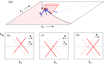
Figure 1: In the presence of static current, the dirac cone, seen in panel (a) on the bare Fermi surface, is shifted in energy and boosted by the wave-vector ${\bf q}$ associated with the super-current. If the current is parallel to ${\bf v}_{f}$ as in (b,c) the net effect is that the cone slides up or down leaving one point of zero energy excitations invariant. If ${\bf q}\perp{\bf v}_{f}$ as in (d) the nodal point is transported along the bare Fermi surface. As shown in panel (a) there is a continuous range of currents ${\bf q}$ that lead to a zero energy peak on each point of the bare Fermi surface. This pile up of spectral weight results in a singular peak at zero energy on the Fermi surface.

In the spirit of refs. [FranzMillis, ; Volovik, ] we will approximate (1) by an average over a distribution of uniform currents. This amounts to a semiclassical approximation valid if spatial variations of the current over a Fermi wavelength are small (i.e. $k_{f}\xi\gg 1$). Interference effects due to coherent scattering of quasi-particles by vortices are neglected in this scheme, which is justified at the temperatures of interest in the normal state.

With these approximations, the spectral function on the two dimensional plane is given by:

$$A(\mathbf{k},{\omega})=\int d^{2}qP(\mathbf{q})A_{\mathbf{q}}(\mathbf{k},{\omega}).$$ (2)

Here $A_{\mathbf{q}}(\mathbf{k},{\omega})$ is the spectral function in the presence of a uniform supercurrent parameterized by a wave-vector $\mathbf{q}$. Such current corresponds to a pairing field that depends on the center of mass coordinate of the pair as ${\Delta}_{\bf k}e^{i2\mathbf{q}\cdot\mathbf{R}}$.

We may now use the standard BCS formalism in order to calculate $A_{\mathbf{q}}(\mathbf{k},{\omega})$ for a given supercurrent $\mathbf{q}$. This is easily seen to be

$$A_{\mathbf{q}}(\mathbf{k},{\omega})=|u_{\mathbf{k}-\mathbf{q}}|^{2}{\delta}({\omega}-E_{\mathbf{k}-\mathbf{q}}(\mathbf{q}))+|v_{\mathbf{k}-\mathbf{q}}|^{2}{\delta}({\omega}+E_{\mathbf{q}-\mathbf{k}}(\mathbf{q}))$$ (3)

and the quasi-particle dispersion to leading order in $\mathbf{q}$ is given by

$$E_{\bf k}(\mathbf{q})\approx\mathbf{v}_{f}(\mathbf{k})\cdot\mathbf{q}+\sqrt{\xi_{\bf k}^{2}+{\Delta}_{\bf k}^{2}}.$$ (4)

for $\mathbf{k}$ near the bare Fermi surface, defined by $\xi_{\mathbf{k}_{f}}={\epsilon}_{\mathbf{k}_{f}}-\mu=0$. To this order in $\mathbf{q}$, the coherence factors $u_{\bf k}$ and $v_{\bf k}$ are unchanged by the current, that is $|u_{\bf k}|^{2}=(1+\xi_{\bf k}/\sqrt{\xi_{\bf k}^{2}+{\Delta}_{\bf k}^{2}})/2$, and $|v_{\bf k}|^{2}=1-|u_{\bf k}|^{2}$.

The essential physics leading to emergence of a Fermi surface in the normal state can be understood qualitatively from Eqs. (3) and (4). Fig. 1 shows the dispersion of the quasi-particle peaks in $A_{\bf q}(\mathbf{k},{\omega})$ for different directions of the supercurrent. The momentum of the peak is shifted by $\mathbf{q}$ because of the boost associated with the supercurrent, but its frequency is also ”Doppler shifted” by $\mathbf{v}_{f}\cdot\mathbf{q}$. For a current parallel (or anti-parralel) to $\mathbf{v}_{f}$, this amounts to the dirac cone sliding up (or down) on the slope of the original dispersion as seen in Fig. 1(b,c). The important thing to note is that in both cases there is a zero frequency peak, or ”Fermi point”, whose position is independent of the current. On the other hand, for current perpendicular to $\mathbf{v}_{f}$ there is no doppler shift, and the node is simply transported a distance $\mathbf{q}$ along the Fermi surface (Fig. 1d). In general an arbitrary current $\mathbf{q}$ will always lead to a zero frequency peak located precisely on the bare Fermi surface. The parallel component of $\mathbf{q}$ leaves the zero frequency peak in place on the nodal point, while the perpendicular component transports it on the fermi surface. In fact, as shown in Fig. 1a, for every point on the Fermi surface, there is a continuous range of wave-vectors $\mathbf{q}$ that lead to a zero frequency peak at that point. This pile up is the origin of the zero frequency singularity that develops on the Fermi surface. However, the probability for a current fluctuation with wavevector larger than a typical $q_{0}$ is strongly suppressed in the distribution $P(\mathbf{q})$. Therefore on points of the fermi surface at a distance larger than $q_{0}$ from the node the singularity is multiplied by a very small pre-factor making it essentially unobservable.

We now turn to a systematic derivation of the spectral function using Eqs. (2),(3) and (4). We concentrate on wavevectors $\mathbf{k}$ sufficiently close to the nodes so that we may approximate the dispersion by a Dirac cone. Namely: ${\Delta}_{\bf k}=\mathbf{v}_{\Delta}\cdot(\mathbf{k}-\mathbf{k}_{n})$ and $\xi_{\bf k}=\mathbf{v}_{f}\cdot(\mathbf{k}-\mathbf{k}_{n})$. Let us also change variables from $\mathbf{q}$ to ${\eta}=\mathbf{v}_{f}\cdot\mathbf{q}$ and $\zeta=\mathbf{v}_{\Delta}\cdot\mathbf{q}$. Plugging these definitions to (2) we have

$$A({\bf k},{\omega})={1\over 2}\int d{\eta}d{\zeta}P({\eta},{\zeta}) \sum_{s=\pm 1}\left(1+s{\xi-{\eta}\over\sqrt{(\xi-{\eta})^{2}+({\Delta}-{\zeta})^{2}}}\right){\delta}({\omega}-{\eta}-s\sqrt{(\xi-{\eta})^{2}+({\Delta}-{\zeta})^{2}})$$ (5)

where for notational simplicity we omitted the subscript $\mathbf{k}$ from ${\Delta}_{\bf k}$ and $\xi_{\bf k}$. The distribution $P({\eta},{\zeta})$ is obtained by a simple change of variables from $P(\mathbf{q})$, which is taken to be a gaussian of the form $P(\mathbf{q})=\mathcal{N}\exp(-\frac{\mathbf{q}^{2}}{q_{0}^{2}(T)})$[FranzMillis, ]. We will later discuss the temperature dependence of $q_{0}$.

In Ref. [FranzMillis, ], the integral (15) was approximated by expanding to leading order in ${\eta}/{\Delta}_{\bf k}$ and ${\zeta}/{\Delta}_{\bf k}$. For $\mathbf{k}$ on the Fermi surface far from a gap node this approximation does give the the dominant spectral feature, which in this region is simply a broadened peak at frequency ${\omega}\sim{\Delta}_{\bf k}$. However, the expansion cannot be generally valid for a superconductor with gap nodes, on which these ratios diverge. In particular, it cannot capture the pile up of low energy spectral weight on the Fermi surface due to movement of the Dirac cone in energy and momentum, as illustrated in Fig. 1.

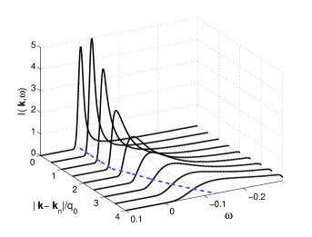
Figure 2: Calculated ARPES energy distribution curves (EDC) for different wave-vectors ${\bf k}$ on the Fermi surface at increasing distance from the node. The curves are obtained by numerical integration of Eq. (20), multiplied by the Fermi function and convolved with a narrow gaussian function to mimic the finite experimental resolution. The dashed line follows the dispersion of the peak, demonstrating the formation of a Fermi arc. Evidently the peak departs from ${\omega}=0$ only at ${\bf k}-{\bf k}_{n}\approx 1.5q_{0}$.

We proceed to evaluate (15) without resorting to an expansion in ${\eta}/{\Delta}_{\bf k}$ and ${\zeta}/{\Delta}_{\bf k}$. In what follows we outline the main steps in the derivation and relegate the details to the online supplementary information. First we transform to the polar coordinates $(r,{\theta})$ defined by $r=\sqrt{(\xi-{\eta})^{2}+({\Delta}-{\zeta})^{2}}$ and $\cos{\theta}=(\xi-{\eta})/r$. This allows to resolve the delta functions in (15) by integrating over $r$. Next to facilitate the angular integration we make another change of variables via ${\alpha}=s\cos{\theta}$. Now, for wavevectors $\mathbf{k}$ on the Fermi surface (i.e. $\xi=0$) the integral reduces to a rather simple form:

$$A(\mathbf{k},{\omega})={\frac{|{\omega}|}{2}}\int_{-1}^{1}d{\alpha}{\frac{(1-{\alpha})^{1/2}}{(1+{\alpha})^{5/2}}}F(|{\omega}|,{\alpha})$$ (6)

where

$$F(|{\omega}|,{\alpha})={\mathcal{N}}\exp\left[{\frac{-|{\omega}|^{2}{\alpha}^{2}}{v_{f}^{2}q_{0}^{2}(1+{\alpha})^{2}}}-{\frac{\left(|{\omega}|\sqrt{\frac{1-{\alpha}}{1+{\alpha}}}+{\Delta}\right)^{2}}{v_{\Delta}^{2}q_{0}^{2}}}\right]$$ (7)

and ${\mathcal{N}}\equiv 1/(\pi v_{f}v_{\Delta}q_{0}^{2})$. For $|{\omega}|\neq 0$, the divergence at ${\alpha}=-1$ in the integrand of (20) is cut off by the first term in the exponent in (7), which effectively introduces a new lower bound to the integral. The singular contribution to the spectral function is now easily evaluated as:

$$A_{sing}(\mathbf{k},{\omega})=A_{0}(v_{\Delta}q_{0})^{-1}e^{-{\Delta}_{\bf k}^{2}/v_{\Delta}^{2}q_{0}^{2}}\sqrt{\frac{v_{f}q_{0}}{|{\omega}|}}$$ (8)

which is the advertised zero frequency singularity. $A_{0}$ is a constant of order unity. Note that the singular contribution comes from ${\alpha}=-1$, which in the original variables corresponds to the range of currents $\mathbf{q}$ defined by the condition $\mathbf{q}\cdot\mathbf{v}_{\Delta}={\Delta}_{\bf k}$. This is precisely the condition for wave-vectors $\mathbf{q}$ illustrated in Fig. 1a that pile up low frequency spectral weight on the point $\mathbf{k}$ on the Fermi surface. If $\mathbf{k}$ is far from the node compared to a typical current fluctuation $q_{0}$, then ${\Delta}/v_{\Delta}q_{0}$ is large and the singularity is strongly suppressed by the exponential pre-factor in (21). Then the dominant spectral feature is a broad peak at frequency ${\omega}\sim{\Delta}$ obtained from taking the saddle point of (20).

The ARPES spectrum is related to the spectral function via $I(\mathbf{k},{\omega})=n_{F}({\omega})A(\mathbf{k},{\omega})$. In Fig. 2 we plot this function for $\mathbf{k}$ points on the Fermi surface at varying distance from the node. The curves are obtained by numerical integration of (20) and the convolution with a narrow gaussian function which mimics the experimental resolution. The overall picture is appealingly similar to what is seen in ARPES experiments in the normal state of under doped cupratesNorman98 ; Kanigel06 . It is seen that the sharp peaks are pinned to zero frequency along a line on the Fermi surface up to a critical distance from the node, which is of the order of $q_{0}$. At larger distance from the node the peak departs from zero frequency, quickly approaches ${\omega}={\Delta}_{\bf k}$ and broadens considerably.

A similar analysis as outlined above can be carried out for points $\mathbf{k}$ on the line of nodes ${\Delta}_{\bf k}=0$ away from the Fermi surface. In this case the singular contribution to the spectral function is given by

$$A_{sing}(\mathbf{k},{\omega})=A_{0}(v_{\Delta}q_{0})^{-1}\sqrt{\frac{v_{f}q_{0}}{|\xi-{\omega}|}},$$ (9)

which appears as a sharp peak dispersing as $\xi_{\bf k}$. This too is in qualitative agreement with ARPES.

We turn to discuss the nature of the phase field in the normal state and the contribution of different types of fluctuations to the electron spectral function. The phase field of a fluctuating 2d superconductor can be decomposed into a longitudinal (non singular) part and a transverse, or vortex contribution. These components are governed by independent actions in the long wavelength limit.

Longitudinal phase fluctuations – These fluctuations may be treated at the gaussian level. Physically they correspond to Josephson plasmons in the d-wave superconductor, which were studied in detail by Paramekanti et al [Randeria, ]. The structure of their spectrum in a layered system is as follows. At low momenta there is a wide regime of linear dispersion, with a small plasmon gap ${\omega}_{pc}$ due to the c-axis Josephson coupling. Experimentally, $\omega_{pc}\approx 8-10$K in Bi2212caxis1 ; caxis2 ; caxis3 , which is lower than typical temperatures of interest in the normal state of lightly underdoped cuprates. we shall therefore neglect this gap. At the high momentum side, the linear plasmon dispersion terminates at a characteristic energy scale $\omega_{p}$ at $q\sim\pi/\xi$. In the cuprates ${\omega}_{p}$ is a high energy scale of order a few eV. Therefore, quantum dynamics of the plasmons must be taken into account fully at the temperatures of interest.

How do these fluctuations affect the fermion spectral function? The most relevant coupling between the Dirac Fermions and the longitudinal phase fluctuations is the current-current couplingDorsey of the form $\mathbf{v}_{f}\cdot\nabla{\varphi}\bar{\psi}_{\sigma}\psi_{\sigma}$. The scaling dimension of this coupling is easily seen to be $-1/2$ making it irrelevant at low energies. Further scaling arguments, and direct calculation, show that the life-time of quasi-particles due to this coupling diverges at low energies as $1/{\tau}\sim({\epsilon}-{\epsilon}_{F})^{2}$. At finite temperature, this will be cut off at $T^{2}$, which gives thermal broadening of the quasi-particles. However a Fermi arc does not form due to coupling to the longitudinal phase fluctuations.

Transverse phase fluctuations– The fluctuations considered in the calculation of the electronic Green’s function (1) are the transverse (vortex) contribution. Vortices are macroscopic objects whose motion is expected to be overdamped. This picture is supported by the fact that the measured Nernst signal and diamagnetism in underdoped cupratesOng are consistent with the predictions from a classical $x-y$ model with overdamped dynamicsPodolsky . In writing (1) as a static average, we assumed this dynamics to be sufficiently slow on quasi-particle timescales.

The arc length at $T>T_{c}$ is of order $q_{0}(T)={\langle\nabla{\varphi}_{\perp}^{2}\rangle}^{1/2}$. That is, the width of the of the transverse current distribution, which we shall calculate within the classical two dimensional $x-y$ model. We note that in the equivalent coulomb gas model, $q_{0}$ is related to the vortex density correlation: $q_{0}^{2}=(4\pi^{2}/\Omega)\sum_{\bf q}{\langle n(\mathbf{q})n(-\mathbf{q})\rangle}/\mathbf{q}^{2}$.

This quantity was previously estimatedDorsey ; FranzMillis in the high temperature limit using the Debye-Hückel approximationHalperinNelson . Here we present a different calculation of $q_{0}\left(T\right)$, using a variational approach. Our result coincides with the Debye-Hückel approximation at high temperature, but can also be used at lower temperatures, closer to $T_{BKT}$. First we carry out the usual mapping of the coulomb gas onto the Sine-Gordon model:

$$S_{SG}=\int d^{2}x\left[\frac{1}{2}\frac{1}{4\pi^{2}K}\left(\nabla\theta\right)^{2}-\frac{2y}{\xi_{c}^{2}}\cos\left[\theta\left(\mathbf{x}\right)+\mu_{v}\left(\mathbf{x}\right)\right]\right]$$ (10)

Here $K=J/T$ is the bare phase stiffness of the original $x-y$ model, $y=\exp(-E_{c}/T)$ where $E_{c}$ is the vortex core energy, and $\xi_{c}$ the core size. $\mu_{v}\left(\mathbf{x}\right)$ is a local chemical potential that couples to the vortices, and allows the calculation of vortex density correlations. We shall now apply the self consistent harmonic approximation (SCHA), which is known to give good results for the correlations in the normal (i.e. gapped) phase Giamarchi . In this approach, the cosine term in (10) is replaced by a quadratic mass term $\frac{1}{2}m^{2}{\theta}^{2}$. The mass is determined by minimizing the variational free energy $F_{0}+T{\langle S-S_{0}\rangle}_{0}$, where $F_{0}$ is the free energy of the quadratic variational action $S_{0}$ and ${\langle\rangle}_{0}$ denotes a thermal average with respect to $S_{0}$. Given the solution $m\left(T\right)=\frac{\pi}{\xi_{c}}\left(8yK\right)^{\frac{1}{2\left(1-\frac{\pi K}{2}\right)}}$, it is now straight forward to compute $q_{0}$ within the variational action.

$$q_{0}^{2}\left(T\right) = \frac{(4\pi y)^{2}}{\xi_{c}^{2}}\left(m\xi_{c}\right)^{2\pi K}$$

$$\times\int_{1}^{\infty}drr\ln r\sinh\left[2\pi Kf\left(m\xi_{c}r\right)\right]$$

$$f\left(m\left|\mathbf{x}\right|\right) = \int_{\left|\mathbf{q}\right|<\frac{\pi}{\xi_{c}}}\frac{d^{2}q}{2\pi}\frac{e^{i\mathbf{q}\cdot\mathbf{x}}}{\mathbf{q}^{2}+m^{2}},$$ (11)

Eq. (36) can be shown to be of the Debye-Hückel form in the high temperature limit.

The parameters $J$, $E_{c}$, and $\xi_{c}$ that control the temperature dependence of $q_{0}$, are not easily connected to observable properties of the cuprates. The parameter $J$ is the bare superfluid stiffness of the $x-y$ model. Nevertheless, in a d-wave superconductor it is expected to be temperature dependant $J(T)=J(0)-AT$ due to physics that lies out side of the pure $x-y$ model, namely depletion of the condensate by quiasiparticles at the gap nodesLeeWen . In the normal phase, the temperature dependence may well be more complicated because of the emergent finite density of states at zero energy. However, to leading order in the current fluctuations we may assume that the linear decrease of $J$ persists in the normal state. We take the parameter $A$ from experiments, that measure the leading temperature dependence of the superfluid densityBoyce . Note the distinction between $J(T)$ which is the bare stiffness of the $x-y$ model and the macroscopic stiffness, which vanishes in the normal state due to proliferation of vortices.

The results of the calculation of the arc length (36) are plotted in Fig. 3 for a range of values of $E_{c}/T_{BKT}$. We assumed that $\xi_{c}=5a$. Near $T_{BKT}$, $q_{0}\left(T\right)$ is exponentially suppressed. At higher temperatures, there is a region where $q_{0}$ increases rapidly due to the proliferation of free vortices, followed by a roughly linear increase region. Since we have assumed that $J(T)=J(0)-AT$, the bare stiffness vanishes at some temperature (which is about $3T_{BKT}$ for our chosen value of $A=0.3$). At this temperature $q_{0}(T)$ diverges logarithmically, and the continuum description of the $x-y$ model breaks down. The temperature dependence of the bare stiffness $J$ above $T_{c}$ in the cuprates is not clear, even though there is some evidence that it continues to decay linearly over a considerable rangeCorson .

In our treatment, we have neglected the inter-plane Josephson coupling. This coupling becomes relevant at some $T_{c}>T_{BKT}$, where a phase transition to a three dimensional ordered state occurs. At this temperature, our treatment of a two dimensional $x-y$ model is no longer valid, vortex formation is strongly suppressed, and we expect $q_{0}\left(T\right)$ to drop abruptly to zero. Indeed, the observed arc length seems to drop to zero at $T_{c}$ [Kanigel06, ].

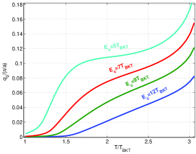
Figure 3: The Fermi arc length is related to the width $q_{0}$ of the current distribution. This is plotted as a function of temperature using eq. (36), for several values of $E_{c}/T_{BKT}$ (see text for details).

Discussion and conclusions – Before concluding let us remark that, we have so far not payed special attention to effects of proximity to the Mott insulating state at half filling. The simplest (though not necessarily the correct) way to include the effect of the strong local repulsion, is via the slave boson mean field theory. Within this approach, the current carried by a quasiparticle is renormalized by a factor ${\alpha}$, which is proportional to the hole doping $x$ [LeeWen, ]. Hence the doppler shift of the quasiparticle dispersion (4) is renormalized by a similar factor, so that ${\bf v}_{f}\cdot{\bf q}\to{\alpha}{\bf v}_{f}\cdot{\bf q}$. This would have a dramatic effect on our earlier considerations. In particular, application of a static current with ${\bf q}$ parallel to ${\bf v}_{f}$ would no longer leave invariant the point of zero energy excitations. Accordingly, the average over the current distribution (3), would not result in a singular peak on the Fermi surface. Specifically, we find the leading edge of the EDC on the Fermi surface behaves as $|{\omega}|$ in this case. It is interesting to note that the same renormalization factor ${\alpha}$, which leads to the present discrepancy of slave boson theory with experiment, is also responsible for its famous failureLeeWen to explain the doping independent slope of the superfluid density with temperatureBoyce .

To summarize, we have shown that destruction of a $d$-wave superconductor by proliferation of thermal vortices must be accompanied by formation of at least a partial fermi surface. We argued that this phenomenon is fundamental to the appearance of Fermi arcs in the normal state of underdoped cupratesNorman98 , and may partially explain their evolution with temperatureKanigel06 . The main results rely on two central assumptions. The first is that vortices are purely thermal and their quantum dynamics may be neglected. The second is the calculation the fermion spectral function in the presence of static vortices within a semiclassical approximation along the lines of [Volovik, ]. The semiclassical approximation was tested in numerical simulationsMarinelli , which verified that it is controlled by the small parameter $v_{\Delta}/v_{f}$. It therefore seems safe to apply the semiclassical approach to the high $T_{c}$ cuprate superconductors, except in the very underdoped regime.

In extremely underdoped materials quantum dynamics of the vortices is also expected to be increasingly important, in violation of our first assumption. Indeed, the onset of superconductivity possibly corresponds to a quantum phase transition, driven by fluctuating quantum vorticesTesanovich ; Sachdev . An important open question is how the normal state we describe, that arises in a thermal vortex liquid, evolves to the highly quantum regime near the critical doping for the onset of superconductivity.

Acknowledgements We are grateful to E. Demler, A. Kanigel, S. Kivelson, A. Paramekanti, and D. Podolsky for illuminating discussions. This research was supported in part by the NSF under Grant No. PHY05-51164 and the U.S.-Israel binational science foundation.

Supplementary information

I Derivation of the Angle resolved Photoemission (ARPES) weight

I.1 Static current

A static current is parameterized by a wave-vector ${\bf q}$ that can be ascribed to a twist in the order parameter, or to the hopping matrix elements of the Hamiltonian as an external vector potential. The two descriptions are related by a simple gauge transformation. The ARPES spectrum in absence of perpendicular magnetic field is given by the gauge invariant Green’s function

$$I({\bf k},{\omega})=i\int d{\bf r}dtG^{<}_{{\sigma}{\sigma}}({\bf r},t)\exp\left(+i{\bf k}\cdot{\bf r}+i{\omega}t-i\int_{0}^{{\bf r}}{\bf A}\cdot{\bf dl}\right)$$ (12)

where $G^{<}_{{\sigma}{\sigma}}({\bf r},t)={\langle c^{\dagger}_{{\sigma},0}(0)c{{}^{\vphantom{\dagger}}}_{{\sigma},{\bf r}}(t)\rangle}$. We induce a current using the gauge ${\bf A}={\bf q}$, for which

$$I_{\bf q}({\bf k},{\omega})=\int dte^{i{\omega}t}{\langle c^{\dagger}_{{\sigma},{\bf k}-{\bf q}}(0)c{{}^{\vphantom{\dagger}}}_{{\sigma},{\bf k}-{\bf q}}(t)\rangle}$$ (13)

Note that this is simply the equilibrium expression for $G^{<}$, boosted by momentum ${\bf q}$. We express (13) in terms of the Bogoliubov operators ${\alpha}_{\bf k}$ that diagonalize the Hamiltonian:

$$I_{\bf q}({\bf k},{\omega}) = |u_{{\bf k}-{\bf q}}|^{2}{\langle{\alpha}^{\dagger}_{{\bf k}-{\bf q},{\uparrow}}{\alpha}{{}^{\vphantom{\dagger}}}_{{\bf k}-{\bf q},{\uparrow}}\rangle}{\delta}({\omega}-E_{{\bf k}-{\bf q}}({\bf q}))+|v_{{\bf k}-{\bf q}}|^{2}{\langle{\alpha}{{}^{\vphantom{\dagger}}}_{-{\bf k}+{\bf q},{\downarrow}}{\alpha}^{\dagger}_{-{\bf k}+{\bf q},{\downarrow}}\rangle}{\delta}({\omega}+E_{{\bf q}-{\bf k}}({\bf q}))$$ (14)

$$= n_{F}({\omega})\Big{(}|u_{{\bf k}-{\bf q}}|^{2}{\delta}({\omega}-E_{{\bf k}-{\bf q}}({\bf q}))+|v_{{\bf k}-{\bf q}}|^{2}{\delta}({\omega}+E_{{\bf q}-{\bf k}}({\bf q}))\Big{)}$$

$$= n_{F}({\omega})A_{{\bf q}}({\bf k},-{\omega}).$$

Here $E_{\bf k}({\bf q})={\bf v}_{f}({\bf k})\cdot{\bf q}+\sqrt{\xi_{\bf k}^{2}+{\Delta}_{\bf k}^{2}}$ is the quasi-particle spectrum to leading order in the current. Note that the coherence factors $u_{\bf k}$ and $v_{\bf k}$ are unchanged by the current to this order in ${\bf q}$. That is, $|u_{\bf k}|^{2}=(1+\xi_{\bf k}/E_{\bf k}(0))/2$ and $|v_{\bf k}|^{2}=(1-\xi_{\bf k}/E_{\bf k}(0))/2$.

I.2 Fluctuating current

As we discuss in the paper, the spectral function in the presence of the phase fluctuations is obtained by averaging (14) over a distribution of static currents. This leads to the following integral:

$$A({\bf k},{\omega})={1\over 2}\int d{\eta}d{\zeta}P({\eta},{\zeta})\sum_{s=\pm 1}\left(1+{s(\xi-{\eta})\over\sqrt{(\xi-{\eta})^{2}+({\Delta}-{\zeta})^{2}}}\right){\delta}({\omega}-{\eta}-s\sqrt{(\xi-{\eta})^{2}+({\Delta}-{\zeta})^{2}}),$$ (15)

where we have denoted: ${\Delta}\equiv\mathbf{v}_{\Delta}\cdot(\mathbf{k}-\mathbf{k}_{n})$, $\xi\equiv\mathbf{v}_{f}\cdot(\mathbf{k}-\mathbf{k}_{n})$, ${\eta}=\mathbf{v}_{f}\cdot\mathbf{q}$, and $\zeta=\mathbf{v}_{\Delta}\cdot\mathbf{q}$. The current distribution is assumed to be gaussian, such that

$$P({\eta},{\zeta})={1\over\pi v_{f}v_{\Delta}q_{0}^{2}}\exp\left(-{{\eta}^{2}\over v_{f}^{2}q_{0}^{2}}-{{\zeta}^{2}\over v_{\Delta}^{2}q_{0}^{2}}\right)$$ (16)

To compute (15) we change to the polar coordinates $r\cos{\theta}=\xi-{\eta}$, $r\sin{\theta}={\Delta}-{\zeta}$. Then (15) takes the form

$$A({\bf k},{\omega})={1\over 2}\int d{\theta}drr{\tilde{P}}_{\xi,{\Delta}}(r,{\theta})\sum_{s=\pm 1}(1-s\cos{\theta}){\delta}\left({\omega}-\xi+sr(1+s\cos{\theta})\right)$$ (17)

where ${\tilde{P}}_{\xi,{\Delta}}(r,{\theta})\equiv P(\xi-r\cos{\theta},{\Delta}-r\sin{\theta})$. Integrating over $r$ to resolve the delta functions and changing variables to ${\alpha}=s\cos{\theta}$ we have

$$A({\bf k},{\omega})={1\over 2}\int_{-1}^{1}d{\alpha}{(1-{\alpha})^{1/2}\over(1+{\alpha})^{5/2}}\left\{({\omega}-\xi)\Theta({\omega}-\xi)F_{\xi,-{\Delta}}({\omega}-\xi,{\alpha})+(\xi-{\omega})\Theta(\xi-{\omega})F_{\xi,{\Delta}}({\omega}-\xi,{\alpha})\right\},$$ (18)

where

$$F_{\xi,{\Delta}}({\omega}-\xi,{\alpha})={1\over\pi v_{f}v_{\Delta}q_{0}^{2}}\exp\left\{-{\left(({\omega}-\xi){{\alpha}\over 1+{\alpha}}+\xi\right)^{2}\over v_{f}^{2}q_{0}^{2}}-{\left(({\omega}-\xi)\sqrt{1-{\alpha}\over 1+{\alpha}}+{\Delta}\right)^{2}\over v_{\Delta}^{2}q_{0}^{2}}\right\}.$$ (19)

For wave-vectors ${\bf k}$ on the Fermi surface we plug $\xi=0$ into (18) and (19). In this case $F_{0,-{\Delta}}({\omega},{\alpha})=F_{0,{\Delta}}(-{\omega},{\alpha})$ and therefore (18) is reduced to

$$A({\bf k},{\omega})={|{\omega}|\over 2}\int_{-1}^{1}d{\alpha}{(1-{\alpha})^{1/2}\over(1+{\alpha})^{5/2}}F_{0,{\Delta}}(|{\omega}|,{\alpha})$$ (20)

The divergence at ${\alpha}=-1$ is cutoff by the first term in the exponent of the distribution $F_{0,{\Delta}}(|{\omega}|,{\alpha})$ which leads to the singular contribution at zero frequency:

$$A_{sing}({\bf k},{\omega})=(v_{\Delta}q_{0})^{-1}e^{-{\Delta}_{\bf k}^{2}/v_{\Delta}^{2}q_{0}^{2}}\sqrt{v_{f}q_{0}\over|{\omega}|}$$ (21)

on the other hand, on the nodal line (${\Delta}_{\bf k}=0$) (18) simplifies to

$$A({\bf k},{\omega})={1\over 2}|{\omega}-\xi|\int_{-1}^{1}d{\alpha}{(1-{\alpha})^{1/2}\over(1+{\alpha})^{5/2}}F_{\xi,0}({\omega}-\xi,{\alpha})$$ (22)

Again the divergence of the integral is cut off by the distribution function. Now the peak is at non vanishing frequency and it disperses a ${\omega}=\xi_{\bf k}$

$$A_{sing}({\bf k},{\omega})\approx{1\over v_{\Delta}q_{0}}\sqrt{v_{f}q_{0}\over|\xi-{\omega}|}$$ (23)

II Role of longitudinal quantum phase fluctuations

In order to estimate the effect of longitudinal quantum phase fluctuations on the low energy fermion properties, we consider the following model of two dimensional nodal Dirac fermions coupled to gaussian phase fluctuations:

$$S=S_{F}+S_{\theta}+\lambda S_{I}$$ (24)

$$S_{F}=\sum_{j}\int d\tau\int d^{2}x\left[\bar{\Psi}_{j}\left(\partial_{\tau}-\sigma^{z}\mathbf{v}_{F}\cdot\frac{1}{i}\mathbf{\nabla}-\sigma^{x}\mathbf{v}_{\Delta}\cdot\frac{1}{i}\mathbf{\nabla}\right)\Psi_{j}\right]$$ (25)

$$S_{\theta}=\int d\tau\int d^{2}x\left[\frac{1}{V_{0}}\left(\partial_{\tau}\theta\right)^{2}+\Lambda_{0}\left(\nabla\theta\right)^{2}\right]$$ (26)

$$S_{I}=\int d\tau\int d^{2}x\sum_{j}\left[-\frac{\mathbf{v}_{F,j}}{2}\cdot\mathbf{\nabla}\theta\bar{\Psi}_{j}\Psi_{j}\right]$$ (27)

Here $\Psi_{j}=\left(\psi_{j,+,\uparrow},\bar{\psi}_{j,-,\downarrow}\right)$ is the Nambu spinor related to the $j$th pair of nodes at $\pm{\bf k}_{j}$ (hence the index $\pm$ of $\psi$). $\lambda$ is a small parameter. The phase action $S_{\theta}$ is taken to be strictly in 2d, rather than a layered system. This simplification does not change the results below, since the essential property of $S_{\theta}$ is the linear 2d-like dispersion near the origin. As we discussed in the paper, the full layered dispersion is nearly linear near the origin (except for a small gap at $\mathbf{k}=0$ due to the c-axis Josephson coupling, which is negligible at the temperatures of interest here).

$S_{I}$ is the minimal coupling action of the fermions to the phase field, of which we keep only the most relevant term consisting of a current-current coupling.

We will treat $\lambda S_{I}$ perturbatively. The ”engineering” scaling dimensions of the fields can be read off from the fixed point action with $\lambda=0$: $\left[\Psi_{j}\right]=-1$, $\left[\theta\right]=-\frac{1}{2}$. Therefore the scaling dimension of $S_{I}$ is found to be $\left[S_{I}\right]=-\frac{1}{2}+O\left(\lambda\right)$, i.e. it is irrelevant in the weak coupling limit. Physically, this means that the coupling to longitudinal phase fluctuations does not change the low energy spectrum of the fermions. In particular, we can estimate the quasiparticle lifetime due to $S_{I}$. To leading order, $1/\tau\left(E\right)\sim\lambda^{2}$. In order to determine the energy dependence, we can perform an RG transformation that takes $E$ to some fixed energy scale $E_{0}>E$. Under this transformation,

$$\lambda\rightarrow\lambda^{\prime}=\left(\frac{E_{0}}{E}\right)^{-\frac{1}{2}+O\left(\lambda\right)}\lambda$$ (28)

therefore

$$\frac{1}{\tau\left(E_{0}\right)}\sim(\lambda^{\prime})^{2}=\left(\frac{E_{0}}{E}\right)^{-1+O\left(\lambda\right)}\lambda^{2}.$$ (29)

Now, since $1/\tau$ has units of energy, we can scale back to get

$$\frac{1}{\tau\left(E\right)}=\frac{E}{E_{0}}\frac{1}{\tau\left(E_{0}\right)}\sim\left(\frac{E}{E_{0}}\right)^{2-O\left(\lambda\right)}\lambda^{2}$$ (30)

We conclude that for weak coupling $1/\tau\left(E\right)\sim E^{2}$, and the low energy quasiparticles are well defined. A direct evaluation of the leading diagram for $1/{\tau\left(E\right)}$ confirms this result.

III Calculation of the typical current fluctuation

The action for the transverse (vortex) part of the phase field in the 2d $x-y$ model is the form of a Coulomb gas model, which can be mapped onto the Sine-Gordon model

$$S_{SG}=\int d^{2}x\left[\frac{1}{2}\frac{1}{4\pi^{2}K}\left(\nabla\theta\right)^{2}-\frac{2y}{\xi_{c}^{2}}\cos\left[\theta\left(\mathbf{x}\right)+\mu_{v}\left(\mathbf{x}\right)\right]\right]$$ (31)

Here $\mu_{v}$ is a vortex chemical potential term, that enables a calculation of vortex density correlations. In particular, the typical current fluctuation is given by

$$q_{0}^{2}=\left\langle\mathbf{\nabla}\varphi_{\perp}^{2}\left(0\right)\right\rangle=\frac{4\pi^{2}}{\Omega}\sum_{\mathbf{q}}\frac{\left\langle n\left(\mathbf{q}\right)n\left(-\mathbf{q}\right)\right\rangle}{\mathbf{q}^{2}}$$ (32)

where $n\left(\mathbf{q}\right)$ is the Fourier transformed vortex density. The vortex density correlation function in real space can be expressed as:

$$\left\langle n\left(\mathbf{q}\right)n\left(-\mathbf{q}\right)\right\rangle = \frac{1}{\xi_{c}^{2}}\int\frac{d^{2}x}{\xi_{c}^{2}}e^{-\mathbf{q}\cdot\mathbf{x}}\left\langle n\left(\mathbf{x}\right)n\left(0\right)\right\rangle$$

$$\left\langle n\left(\mathbf{x}\right)n\left(0\right)\right\rangle = -\left(2y\right)^{2}\left\langle\sin\left[\theta\left(\mathbf{x}\right)\right]\sin\left[\theta\left(0\right)\right]\right\rangle+2y\xi_{c}^{2}\delta\left(\mathbf{x}\right)\left\langle\cos\left[\theta\left(0\right)\right]\right\rangle$$ (33)

The last line is obtained by taking $\mu_{v}$ derivatives of the Sine-Gordon partition function. Charge neutrality of the Coulomb gas model fixes $\int d^{2}x\left\langle n\left(\mathbf{x}\right)n\left(0\right)\right\rangle=0$. Indeed, we see that otherwise $q_{0}^{2}$ (which is proportional to the total electostatic energy) diverges.

In order to calculate (33) in the gapped (disordered) phase, we use the self consistent harmonic approximation. The action (31) is replaced by the quadratic action

$$S_{SCHA}=\frac{1}{4\pi^{2}K}\int d^{2}x\left[\frac{1}{2}\left(\nabla\theta\right)^{2}+\frac{m^{2}}{2}\theta^{2}\right]$$ (34)

$m$ is a variational parameter determined by minimizing the free energy of the system. The optimal value is $m=\frac{\pi}{\xi_{c}}\left(8yK\right)^{\frac{1}{2\left(1-\frac{\pi K}{2}\right)}}$. The calculation of (33) with the action (34) is strait forward, and yields

$$\left\langle n\left(\mathbf{x}\right)n\left(0\right)\right\rangle_{0} = -\left(2y\right)^{2}\left(\xi_{c}m\right)^{2\pi K}\sinh\left[2\pi Kf\left(m\left|\mathbf{x}\right|\right)\right]+A\xi_{c}^{2}\delta\left(\mathbf{x}\right)$$

$$f\left(m\left|\mathbf{x}\right|\right) = \int_{\left|\mathbf{q}\right|<\frac{\pi}{\xi_{c}}}\frac{d^{2}q}{2\pi}\frac{e^{i\mathbf{q}\cdot\mathbf{x}}}{\mathbf{q}^{2}+m^{2}}$$ (35)

Here $A=2y\left\langle\cos\left[\theta\left(\mathbf{x}_{1}\right)\right]\right\rangle$. Instead of calculating $A$ directly, we will adjust it so that (35) satisfies the exact charge neutrality sum rule $\int d^{2}x\left\langle n\left(\mathbf{x}\right)n\left(0\right)\right\rangle=0$. In the high temperature ($K\rightarrow 0$) limit, (35) reduces to the Debye-Hückel form.

Plugging (35) into (32) and using $\int\frac{d^{2}q}{2\pi}\frac{e^{i\mathbf{q\cdot x}}}{\mathbf{q}^{2}}=\ln\frac{L}{\left|\mathbf{x}\right|}$ (where $L$ is the system size, which is taken to infinity at the end of the calculation), we finally get

$$q_{0}^{2}\left(T\right)=\frac{\left(4\pi y\right)^{2}}{\xi_{c}^{2}}\left(\xi_{c}m\right)^{2\pi K}\int_{1}^{\infty}drr\ln r\sinh\left[2\pi Kf\left(m\xi_{c}r\right)\right]$$ (36)

References

- (1) Y. J. Uemura et al, Phys. Rev. Lett. 62, 2317 (1989).
- (2) V. J. Emery and S. A. Kivelson, Nature 374, 434 (2002).
- (3) M. Franz and A. J. Millis, Phys. Rev. B 58, 14572 (1998).
- (4) H-J. Kwon and A. T. Dorsey, Phys. Rev. B 59, 6438 (1999)
- (5) M. R. Norman et al, Nature 392, 157–160 (1998).
- (6) A. Kanigel et al, Nature Phys. 2, 447 (2006)
- (7) G. E. Volovik, JETP Lett. 58, 469 (1993).
- (8) C. M. Varma and L. Zhu, cond-mat/0607777.
- (9) A. Paramekanti and E. Zhao, Phys. Rev. B 75, 140507 (2007)
- (10) E.-A. Kim, M. Lawler, P. Oreto, E. Fradkin, and S. Kivelson, unpublished.
- (11) A. Paramekanti, M. Randeria, T. V. Ramakrishnan and S. S. Mandal, Phys. Rev. B 62, 6786 (2000).
- (12) T. Eckl, D. J. Scalapino, E. Arrigoni, and W. Hanke, Phys. Rev. B 66, 140510 (2002)
- (13) K.C. Tsui, N.P. Ong, and J.B. Peterson, Phys. Rev. Lett. 76, 819 (1996).
- (14) Mallozzi, J. Corson, J. Orenstein, J.N. Eckstein, and I. Bozovic, J. Phys. Chem. Solids 59, 2095 (1998).
- (15) K. Kadowaki, I. Kakeya, and K. Kindo, Europhys. Lett. 42, 203 (1998).
- (16) B. I. Halperin and D. R. Nelson, J. Low Temp. Phys. 36, 599 (1979).
- (17) Y. Wang, L. Li, and N.P. Ong, Phys. Rev. B 73, 024510 (2006)
- (18) D. Podolsky, S. Raghu and A. Vishwanath, cond-mat/0612096 (Preprint).
- (19) For an application of the SCHA to the Sine-Gordon model, see T. Giamarchi, Quantum Physics in One Dimension, Oxford university press (2004).
- (20) P. A. Lee and X-G. Wen, Phys. Rev. Lett. 78, 4111 (1997).
- (21) J. Corson, R. Mallozzi, J. Orenstein, J. Eckstein, and I. Bozovic, 1999, Nature 398, 221.
- (22) B. R. Boyce, J. Skinta, and T. Lemberger, Physica C 341-348, 561 (2000).
- (23) L. Marinelli, B. I. Halperin, and S. H. Simon, Phys. Rev. B 62, 3488 (2000).
- (24) Z. Tesanovic, Phys. Rev. Lett. 9, 217004 (2004).
- (25) L. Balents et al, Phys. Rev. B 71, 144508 (2005).