Application of Girsanov Theorem to Particle Filtering of Discretely Observed Continuous-Time Non-Linear Systems

Abstract

This article considers the application of particle filtering to continuous-discrete optimal filtering problems, where the system model is a stochastic differential equation, and noisy measurements of the system are obtained at discrete instances of time. It is shown how the Girsanov theorem can be used for evaluating the likelihood ratios needed in importance sampling. It is also shown how the methodology can be applied to a class of models, where the driving noise process is lower in the dimensionality than the state and thus the laws of state and noise are not absolutely continuous. Rao-Blackwellization of conditionally Gaussian models and unknown static parameter models is also considered.

1 Introduction

This article considers the application of sequential importance sampling based particle filtering (see, e.g. Kitagawa, 1996; Doucet et al., 2001) to continuous-discrete filtering problems (Jazwinski, 1970), where the dynamic model is a stochastic differential equation of the form

$$\mathrm{d}\mathbf{x}(t)=\mathbf{f}(\mathbf{x}(t),t)\,\mathrm{d}t+\mathit{L}(t)\,\mathrm{d}\mathrm{\boldsymbol{\beta}}(t),$$ (1)

where $\mathbf{x}(t)\in\mathbb{R}^{n}$ is the state, $\mathbf{f}:\mathbb{R}^{n}\times\mathbb{R}_{+}\mapsto\mathbb{R}^{n}$ is the drift term, $\mathit{L}(t):\mathbb{R}^{n}\times\mathbb{R}_{+}\mapsto\mathbb{R}^{n\times s}$ is the dispersion matrix, and $\mathrm{\boldsymbol{\beta}}(t)\in\mathbb{R}^{s}$ is an $s$-dimensional Brownian motion with diffusion matrix $\mathit{Q}(t)$. It is assumed that the required conditions (Karatzas and Shreve, 1991; Øksendal, 2003) for existence of a strong solution to the equation are satisfied. In this article, we first consider the case where the dimensionality of the state is the same as the dimensionality of the Brownian motion, that is, where $s=n$. We also extend the results to the singular case where the dimensionality of the Brownian motion is less than the dimensionality of the state, that is, where $s<n$.

The likelihood of a measurement $\mathbf{y}_{k}$ is modeled by a probability density, which is a function of the state at time $t_{k}$:

$$\mathbf{y}_{k}\sim p(\mathbf{y}_{k}\,|\,\mathbf{x}(t_{k})).$$ (2)

The purpose of the Bayesian optimal continuous-discrete filter is to compute the posterior distribution (or at least the posterior mean) of the current state $\mathbf{x}(t_{k})$ given the measurements up to the current time, that is (Jazwinski, 1966, 1970)

$$p(\mathbf{x}(t_{k})\,|\,\mathbf{y}_{1},\ldots,\mathbf{y}_{k}).$$ (3)

This kind of continuous-discrete filtering models are common in engineering applications, especially in the fields of navigation, communication and control (Bar-Shalom et al., 2001; Grewal et al., 2001; Stengel, 1994; Van Trees, 1968, 1971). In these applications, the dynamic system or a physical phenomenon can be modeled as a stochastic differential equation, which is observed at discrete instances of time with certain physical sensors. The purpose of the filtering or recursive estimation is to infer the state of the system from the observed noisy measurements.

In this article, novel measure transformation based methods for continuous-discrete sequential importance resampling (see, e.g. Gordon et al., 1993; Kitagawa, 1996; Pitt and Shephard, 1999; Doucet et al., 2001; Ristic et al., 2004) are presented. Some of the methods have already been presented in (Särkkä, 2006b, a), but here the methods are significantly extended. The methods are based on transformations of probability measures by the Girsanov theorem (Kallianpur, 1980; Karatzas and Shreve, 1991; Øksendal, 2003), which is a theorem from mathematical probability theory. The theorem can be used for computing likelihood ratios of stochastic processes. It states that the likelihood ratio of a stochastic process and Brownian motion, that is, the Radon-Nikodym derivative of the measure of the stochastic process with respect to the measure of Brownian motion, can be represented as an exponential martingale which is the solution to a certain stochastic differential equation.

Measure transformation based approaches are particularly successful in continuous time filtering (Kallianpur, 1980), but are less common in continuous-discrete filtering. The general idea of using the Girsanov theorem in importance sampling of SDEs has been presented, for example, in Kloeden and Platen (1999). Similar ideas have also been presented by several authors (Ionides, 2004; Crisan and Lyons, 1999; Crisan et al., 1998; Crisan, 2003; Moral and Miclo, 2000).

Beskos et al. (2006) considers exact Monte Carlo simulation of a restricted class of diffusion models, which are observed at discrete instances of time without any observation error. As shown in the discussion of the article, the observation errors can be included in the model. Fearnhead et al. (2007) introduces particles filters for a class of multidimensional diffusion processes, and the used Monte Carlo sampling methodology is based on the exact simulation framework of Beskos et al. (2006). The difference to the present methodology is that the methods of Fearnhead et al. (2007) are not based on time-discretization.

Durham and Gallant (2002) considers simulated maximum likelihood estimation of parameters of discretely observed stochastic stochastic differential equations, where all or some of the components are perfectly observed. The methods are based on approximating the transition densities of the processes and modeling the unobserved sample paths as latent data. Golightly and Wilkinson (2006) applies similar methodology to sequential estimation of state and parameters of stochastic differential equation models. Chib et al. (2004) considers MCMC based simulation of diffusion driven state space models. In the article, it is also shown how the methodology can be applied to particle filtering of such models.

The advantages of the method proposed here over the previously proposed methods are:

• Unlike many measure transformation based approaches the methodology presented here is not restricted to one-dimensional or to SDE models with non-singular dispersion or diffusion matrices. The state dimensionality can be higher than the dimensionality of the driving Brownian motion, which is equivalent to the case that the dispersion/diffusion matrix is singular.

• The SDE formulation of the likelihood ratio computation allows efficient numerical solving of the problem. In particular, simulation based approaches (Kloeden and Platen, 1999) can be applied. Of course, any other numerical methods for SDEs could be applied as well.

• Dispersion (and diffusion) matrices may depend on time, that is, the driving process can be time inhomogeneous.

• The observation errors can be easily modeled and the model flexibility is the same as with discrete-time particle filtering.

• Efficient importance distributions and Rao-Blackwellization can be easily used for improving the efficiency of the sampling.

2 Continuous-Discrete Sequential Importance Resampling

2.1 Filtering Models

We shall concentrate into the following four forms of dynamic models:

1. Non-singular models, where the dispersion matrices are invertible and thus the dimensionality of the process is the same as of the driving Brownian motion. The advantage of this kind of processes is that their likelihood ratios can be easily evaluated using the Girsanov theorem, but the problem is that they are too restricted models for many applications.

2. Singular models, where there is non-singular type of model, which is embedded inside a deterministic differential equation model and thus the joint model is singular because the dimensionality of the process is higher than of the driving Brownian motion. This kind of models are typical in navigation and stochastic control applications, where the deterministic part is typically plain integral operator. Because the outer operator is deterministic, the likelihood ratios of processes are determined by the inner stochastic processes alone and thus importance sampling of this kind of process is very similar to the processes of non-singular type above.

3. Conditionally Gaussian models, where a linear stochastic differential equation is driven by a model of the non-singular or singular type above. This kind of models can be handled such that we only sample the inner process and integrate the linear part using the Kalman filter. This way we can form a Rao-Blackwellized estimate, where the probability density is approximated by a mixture of Gaussian distributions.

4. Conjugate static parameter models, where the model contains a static parameter in such conjugate form that certain marginalizations can be analytically evaluated. This result in particle filter, where only the dynamic state is sampled and the sufficient statistics of the static parameter are evaluated at each update stage.

2.2 Non-Singular and Singular Models

Assume that the filtering model is of the form

$$\begin{split}\mathrm{d}\mathbf{x}&=\mathbf{f}(\mathbf{x},t)\,\mathrm{d}t+\mathit{L}(t)\,\mathrm{d}\mathrm{\boldsymbol{\beta}}\\ \mathbf{y}_{k}&\sim p(\mathbf{y}_{k}\,|\,\mathbf{x}(t_{k})),\end{split}$$ (4)

where $\mathrm{\boldsymbol{\beta}}(t)$ is a Brownian motion with positive definite diffusion matrix $\mathit{Q}(t)$, $\mathit{L}(t)$ is an invertible matrix for all $t\geq 0$ and the initial conditions are $\mathbf{x}(0)\sim p(\mathbf{x}(0))$. Further assume that we have constructed an importance process $\mathbf{s}(t)$, which is defined by the SDE

$$\mathrm{d}\mathbf{s}=\mathbf{g}(\mathbf{s},t)\,\mathrm{d}t+\mathit{B}(t)\,\mathrm{d}\mathrm{\boldsymbol{\beta}},$$ (5)

and which has a probability law that is a rough approximation to the filtering (or smoothing) distribution of the model (4), at least at the measurement times. The matrix $\mathit{B}(t)$ is also assumed to be invertible for all $t\geq 0$. Note that at this point we do not want to restrict the matrix $\mathit{B}(t)$ to be the same as $\mathit{L}(t)$, because this allows usage of greater class of importance processes as shall be seen later in this article.

Now it is possible to generate a set of importance samples from the conditioned (i.e., filtered) process $\mathbf{x}(t)$, which is conditional to the measurements $\mathbf{y}_{1:k}$ using $\mathbf{s}(t)$ as the importance process. The motivation of this is that because the process $\mathbf{s}(t)$ already is an approximation to the optimal result, using it as the importance process is likely to produce a less degenerate particle set and thus more accurate presentation of the filtering distribution.

Because the matrices $\mathit{L}(t)$ and $\mathit{B}(t)$ are invertible, the probability measures of $\mathbf{x}$ and $\mathbf{s}$ are absolutely continuous with respect to the probability measure of the driving Brownian motion $\mathrm{\boldsymbol{\beta}}(t)$ and it is possible to compute likelihood ratio between the target and importance processes by applying the Girsanov theorem. The explicit expression and derivation of this likelihood ratio is given in Theorem A.3 of Appendix A.

The SIR algorithm recursion starts by drawing samples $\{\mathbf{x}^{(i)}_{0}\}$ from the initial distribution and setting $w^{(i)}_{0}=1/N$, where $N$ is the number of Monte Carlo samples. The continuous-discrete SIR filter algorithm then proceeds as follows:

Algorithm 2.1 (CD-SIR I)

Given the importance process $\mathbf{s}(t)$, a weighted set of samples $\{\mathbf{x}^{(i)}_{k-1},w^{(i)}_{k-1}\}$ and the new measurement $\mathbf{y}_{k}$, a single step of continuous-discrete sequential importance resampling can be performed as follows:

1. Simulate $N$ realizations of the importance processes

   $$\mathrm{d}\mathbf{s}^{(i)} =\mathbf{g}(\mathbf{s}^{(i)},t)\,\mathrm{d}t+\mathit{B}(t)\,\mathrm{d}\mathrm{\boldsymbol{\beta}}^{(i)}(t),\quad \mathbf{s}^{(i)}(t_{k-1})=\mathbf{x}^{(i)}_{k-1}$$

   $$\mathrm{d}\mathbf{s}^{*(i)}(t) =\mathit{L}(t)\,\mathit{B}^{-1}(t)\,\mathrm{d}\mathbf{s}^{(i)}(t),\quad \mathbf{s}^{*(i)}(t_{k-1})=\mathbf{x}^{(i)}_{k-1},$$

   from $t=t_{k-1}$ to $t=t_{k}$, where $\mathrm{\boldsymbol{\beta}}^{(i)}(t)$ are independent Brownian motions, and $i=1,\ldots,N$.

2. At the same time, simulate the log-likelihood ratios

   $$\begin{split}\mathrm{d}\Lambda^{(i)}&=\big{\{}\mathbf{f}(\mathbf{s}^{*(i)}(t),t)-\mathit{L}(t)\,\mathit{B}^{-1}(t)\,\mathbf{g}(\mathbf{s}^{(i)}(t),t)\big{\}}^{T}\\ &\quad\times\mathit{L}^{-T}(t)\,\mathit{Q}^{-1}(t)\,\mathrm{d}\mathrm{\boldsymbol{\beta}}^{(i)}(t)\\ &-\frac{1}{2}\big{\{}\mathbf{f}(\mathbf{s}^{*(i)}(t),t)-\mathit{L}(t)\,\mathit{B}^{-1}(t)\,\mathbf{g}(\mathbf{s}^{(i)}(t),t)\big{\}}^{T}\\ &\quad\times\big{\{}\mathit{L}(t)\,\mathit{Q}(t)\,\mathit{L}^{T}(t)\big{\}}^{-1}\\ &\quad\times\big{\{}\mathbf{f}(\mathbf{s}^{*(i)}(t),t)-\mathit{L}(t)\,\mathit{B}^{-1}(t)\,\mathbf{g}(\mathbf{s}^{(i)}(t),t)\big{\}}\,\mathrm{d}t,\\ \Lambda^{(i)}(t_{k-1})&=0,\end{split}$$

   from $t=t_{k-1}$ to $t=t_{k}$ and set

   $$\begin{split}\mathbf{x}^{(i)}_{k}&=\mathbf{s}^{*(i)}(t_{k})\\ Z^{(i)}_{k}&=\exp\left\{\Lambda^{(i)}(t_{k})\right\}.\end{split}$$

   Note that the realizations of Brownian motions must be the same as in simulation of the importance processes.

3. For each $i$ compute

   $$\begin{split}w^{(i)}_{k}&=w^{(i)}_{k-1}\,Z^{(i)}_{k}\,p(\mathbf{y}_{k}\,|\,\mathbf{x}^{(i)}_{k}),\end{split}$$

   and re-normalize the weights to sum to unity.

4. If the effective number of particles is too low, perform resampling.

Some practical points about the implementation:

• The importance process $\mathbf{s}(t)$ required by the algorithm can be obtained by using, for example, the extended Kalman filter (EKF). An example of this approach is given in Section 3.1 of this article.

• The simulation of the importance processes and likelihood ratios above can be performed using any of the well known numerical methods for simulation of stochastic differential equations (Kloeden and Platen, 1999). In this article we have used the simple Euler-Maruyama method, which can be considered as a stochastic version of the Euler integration for non-stochastic differential equations.

The class (4) is actually very restricted class of dynamic models, where it is required that the probability law of the state is absolutely continuous with respect to the law of the driving Brownian motion. This kind of models are common in mathematical treatment of stochastic differential equations and such models can be found, for example, in mathematical finance (see, e.g., Karatzas and Shreve, 1991; Øksendal, 2003). However, most of the models used in navigation and telecommunications applications do not fit into this class, and for this reason the results need to be extended.

It is also possible to construct a similar SIR algorithm for more general models, where there is an absolutely continuous type of model, which is embedded inside a deterministic differential equation model. This kind of models are typical in navigation, communication and stochastic control applications (Bar-Shalom et al., 2001; Grewal et al., 2001; Stengel, 1994; Van Trees, 1968, 1971), where the deterministic part is typically a plain integral operator. Because the outer operator is deterministic, the likelihood ratios of processes are determined by the inner stochastic processes alone and thus importance sampling of this kind of process is very similar to sampling of the processes considered above.

Assume that the model is of the form

$$\begin{split}\frac{\mathrm{d}\mathbf{x}_{1}}{\mathrm{d}t}&=\mathbf{f}_{1}(\mathbf{x}_{1},\mathbf{x}_{2},t),\\ \mathrm{d}\mathbf{x}_{2}&=\mathbf{f}_{2}(\mathbf{x}_{1},\mathbf{x}_{2},t)\,\mathrm{d}t+\mathit{L}(t)\,\mathrm{d}\mathrm{\boldsymbol{\beta}}\\ \mathbf{y}_{k}&\sim p(\mathbf{y}_{k}\,|\,\mathbf{x}_{1}(t_{k}),\mathbf{x}_{2}(t_{k})),\end{split}$$ (6)

where $\mathbf{f}_{1}(\cdot)$ and $\mathbf{f}_{2}(\cdot)$ are deterministic functions, $\mathrm{\boldsymbol{\beta}}(t)$ is a Brownian motion, $\mathit{L}(t)$ is invertible matrix and the initial conditions are $\mathbf{x}_{1}(0),\mathbf{x}_{2}(0)\sim p(\mathbf{x}_{1}(0),\mathbf{x}_{2}(0))$. Note that because the dimensionality of Brownian motion is less than of the joint state $(\mathbf{x}_{1}~{}\mathbf{x}_{2})^{T}$ it is not possible to compute the likelihood ratio between the process and Brownian motion by the Girsanov theorem directly.

However, it turns out that if the importance process for $(\mathbf{x}_{1}~{}\mathbf{x}_{2})^{T}$ is formed as follows

$$\begin{split}\frac{\mathrm{d}\mathbf{s}_{1}}{\mathrm{d}t}&=\mathbf{f}_{1}(\mathbf{s}_{1},\mathbf{s}_{2},t)\\ \mathrm{d}\mathbf{s}_{2}&=\mathbf{g}_{2}(\mathbf{s}_{1},\mathbf{s}_{2},t)\,\mathrm{d}t+\mathit{B}(t)\,\mathrm{d}\mathrm{\boldsymbol{\beta}},\end{split}$$ (7)

then the importance weights can be computed in exactly the same way as when forming importance sample of $\mathbf{x}_{2}(t)$ using $\mathbf{s}_{2}(t)$ as the importance process.

The likelihood ratio expression is given in Theorem A.5 of Appendix A. The SIR algorithm is started by first drawing samples from the initial distribution and then for each measurement, the following steps are performed:

Algorithm 2.2 (CD-SIR II)

Given the importance process $\mathbf{s}_{1}(t),\mathbf{s}_{2}(t)$, a weighted set of samples $\{\mathbf{x}^{(i)}_{1,k-1},\mathbf{x}^{(i)}_{2,k-1},w^{(i)}_{k-1}\}$ and the new measurement $\mathbf{y}_{k}$, a single step of continuous-discrete sequential importance resampling can be performed as follows:

1. Simulate $N$ realizations of the importance processes

   $$\frac{\mathrm{d}\mathbf{s}^{(i)}_{1}}{\mathrm{d}t} =\mathbf{f}_{1}(\mathbf{s}^{(i)}_{1},\mathbf{s}^{(i)}_{2},t),\quad \mathbf{s}^{(i)}_{1}(t_{k-1})=\mathbf{x}^{(i)}_{1,k-1}$$

   $$\mathrm{d}\mathbf{s}^{(i)}_{2} =\mathbf{g}_{2}(\mathbf{s}^{(i)}_{1},\mathbf{s}^{(i)}_{2},t)\,\mathrm{d}t+\mathit{B}(t)\,\mathrm{d}\mathrm{\boldsymbol{\beta}}^{(i)}(t),\quad \mathbf{s}^{(i)}_{2}(t_{k-1})=\mathbf{x}^{(i)}_{2,k-1}$$

   $$\frac{\mathrm{d}\mathbf{s}^{*(i)}_{1}}{\mathrm{d}t} =\mathbf{f}_{1}(\mathbf{s}^{*(i)}_{1},\mathbf{s}^{*(i)}_{2},t),\quad \mathbf{s}^{*(i)}_{1}(t_{k-1})=\mathbf{x}^{(i)}_{1,k-1}$$

   $$\mathrm{d}\mathbf{s}^{*(i)}_{2} =\mathit{L}(t)\,\mathit{B}^{-1}(t)\,\mathrm{d}\mathbf{s}_{2},\quad \mathbf{s}^{*(i)}_{2}(t_{k-1})=\mathbf{x}^{(i)}_{2,k-1},$$

2. Simulate the log-likelihood ratios (using the same Brownian motion realizations as above)

   $$\begin{split}\mathrm{d}\Lambda^{(i)}&=\big{\{}\mathbf{f}_{2}(\mathbf{s}^{*(i)}_{1}(t),\mathbf{s}^{*(i)}_{2}(t),t)-\mathit{L}(t)\,\mathit{B}^{-1}(t)\,\mathbf{g}_{2}(\mathbf{s}_{1}^{(i)}(t),\mathbf{s}_{2}^{(i)}(t),t)\big{\}}^{T}\\ &\quad\times\mathit{L}^{-T}(t)\,\mathit{Q}^{-1}(t)\,\mathrm{d}\mathrm{\boldsymbol{\beta}}^{(i)}(t)\\ &-\frac{1}{2}\big{\{}\mathbf{f}_{2}(\mathbf{s}^{*(i)}_{1}(t),\mathbf{s}^{*(i)}_{2}(t),t)-\mathit{L}(t)\,\mathit{B}^{-1}(t)\,\mathbf{g}_{2}(\mathbf{s}_{1}^{(i)}(t),\mathbf{s}^{(i)}_{2}(t),t)\big{\}}^{T}\\ &\quad\times\big{\{}\mathit{L}(t)\,\mathit{Q}(t)\,\mathit{L}^{T}(t)\big{\}}^{-1}\\ &\quad\times\big{\{}\mathbf{f}_{2}(\mathbf{s}^{*(i)}_{1}(t),\mathbf{s}^{*(i)}_{2}(t),t)-\mathit{L}(t)\,\mathit{B}^{-1}(t)\,\mathbf{g}_{2}(\mathbf{s}^{(i)}_{1}(t),\mathbf{s}^{(i)}_{2}(t),t)\big{\}}\,\mathrm{d}t,\\ &\Lambda^{(i)}(t_{k-1})=0,\end{split}$$

   from $t=t_{k-1}$ to $t=t_{k}$ and set

   $$\begin{split}\mathbf{x}^{(i)}_{1,k}&=\mathbf{s}^{*(i)}_{1}(t_{k})\\ \mathbf{x}^{(i)}_{2,k}&=\mathbf{s}^{*(i)}_{2}(t_{k})\\ Z^{(i)}_{k}&=\exp\left\{\Lambda^{(i)}(t_{k})\right\}.\end{split}$$ (8)

3. For each $i$ compute

   $$\begin{split}w^{(i)}_{k}&=w^{(i)}_{k-1}\,Z^{(i)}_{k}\,p(\mathbf{y}_{k}\,|\,\mathbf{x}^{(i)}_{1,k},\mathbf{x}^{(i)}_{2,k}),\end{split}$$ (9)

   and re-normalize the weights to sum to unity.

4. If the effective number of particles is too low, perform resampling.

The importance process $\mathbf{s}(t)$ required by the algorithm can be obtained by using, for example, continuous-discrete EKF and then extracting the estimate of the inner process $\mathbf{s}_{2}(t)$ from the joint estimate.

2.3 Rao-Blackwellization of Conditionally Gaussian Models

Now we shall consider dynamic models, where a linear stochastic differential equation is driven by a singular or non-singular model considered in the previous section. This kind of models can be handled such that only the inner process is sampled and the linear part is integrated out using the continuous-discrete Kalman filter. Then it is possible to form a Rao-Blackwellized estimate, where the probability density is approximated by a mixture of Gaussian distributions. The measurement model is assumed to be of the same form as in previous sections, but linear with respect to the state variables corresponding to the linear part of the dynamic process.

Dynamic models with conditionally Gaussian parts arise, for example, when the measurement noise correlations are modeled with state augmentation (see, e.g., Gelb, 1974). Actually, in this case, the direct application of particle filter without Rao-Blackwellization would be impossible because the measurement model is formally singular. However, the Rao-Blackwellized filter can be easily applied to this kind of models.

Assume that the dynamic model is of the form

$$\begin{split}\mathrm{d}\mathbf{x}_{1}&=\mathbf{F}(\mathbf{x}_{2},\mathbf{x}_{3},t)\,\mathbf{x}_{1}\,\mathrm{d}t+\mathbf{f}_{1}(\mathbf{x}_{2},\mathbf{x}_{3},t)\,\mathrm{d}t+\mathit{V}(\mathbf{x}_{2},\mathbf{x}_{3},t)\,\mathrm{d}\boldsymbol{\eta}\\ \frac{\mathrm{d}\mathbf{x}_{2}}{\mathrm{d}t}&=\mathbf{f}_{2}(\mathbf{x}_{2},\mathbf{x}_{3},t)\\ \mathrm{d}\mathbf{x}_{3}&=\mathbf{f}_{3}(\mathbf{x}_{2},\mathbf{x}_{3},t)\,\mathrm{d}t+\mathit{L}(t)\,\mathrm{d}\mathrm{\boldsymbol{\beta}},\end{split}$$ (10)

where $\boldsymbol{\eta}$ and $\mathrm{\boldsymbol{\beta}}$ are independent Brownian motions with diffusion matrices $\mathit{Q}_{\eta}(t)$ and $\mathit{Q}_{\beta}(t)$, respectively. Also assume that the initial conditions are given as:

$$\begin{split}\mathbf{x}_{1}(0)&\sim\operatorname{N}(\mathbf{m}_{0},\mathbf{P}_{0})\\ \mathbf{x}_{2}(0),\mathbf{x}_{3}(0)&\sim p(\mathbf{x}_{2}(0),\mathbf{x}_{3}(0)),\end{split}$$ (11)

and the initial conditions of $\mathbf{x}_{1}(0)$ are independent from those of $\mathbf{x}_{2}(0)$ and $\mathbf{x}_{3}(0)$.

In this case an importance process can be formed as

$$\begin{split}\mathrm{d}\mathbf{s}_{1}&=\mathbf{F}(\mathbf{s}_{2},\mathbf{s}_{3},t)\,\mathbf{s}_{1}\,\mathrm{d}t+\mathbf{f}_{1}(\mathbf{s}_{2},\mathbf{s}_{3},t)\,\mathrm{d}t+\mathit{V}(\mathbf{s}_{2},\mathbf{s}_{3},t)\,\mathrm{d}\boldsymbol{\eta},\\ \frac{\mathrm{d}\mathbf{s}_{2}}{\mathrm{d}t}&=\mathbf{f}_{2}(\mathbf{s}_{2},\mathbf{s}_{3},t)\\ \mathrm{d}\mathbf{s}_{3}&=\mathbf{g}_{3}(\mathbf{s}_{2},\mathbf{s}_{3},t)\,\mathrm{d}t+\mathit{B}(t)\,\mathrm{d}\mathrm{\boldsymbol{\beta}},\end{split}$$ (12)

with the same initial conditions. In both the original and importance processes, conditionally to the filtration of the second Brownian motion $\mathcal{F}_{t}=\sigma(\mathrm{\boldsymbol{\beta}}(s),0\leq s\leq t)$ and to initial conditions, the law of the first equation is determined by the mean and covariance of the Gaussian process, which is driven by the process $\boldsymbol{\eta}(t)$. Thus, conditionally to $\mathbf{x}_{2}$ and $\mathbf{x}_{3}$ the process $\mathbf{x}_{1}(t)$ is Gaussian for all $t$. The same applies to the importance process.

Now it is possible to integrate out the Gaussian parts of both processes. This procedure results in the following marginalized equations for the original process:

$$\frac{\mathrm{d}\mathbf{m}_{x}(t)}{\mathrm{d}t} =\mathit{F}(\mathbf{x}_{2},\mathbf{x}_{3},t)\,\mathbf{m}_{x}(t)+\mathbf{f}_{1}(\mathbf{x}_{2},\mathbf{x}_{3},t)$$

$$\frac{\mathrm{d}\mathbf{P}_{x}(t)}{\mathrm{d}t} =\mathit{F}(\mathbf{x}_{2},\mathbf{x}_{3},t)\,\mathit{P}_{x}(t)+\mathit{P}_{x}(t)\,\mathit{F}^{T}(\mathbf{x}_{2},\mathbf{x}_{3},t)$$

$$+\mathit{V}(\mathbf{x}_{2},\mathbf{x}_{3},t)\,\mathbf{Q}_{\eta}(t)\,\mathit{V}^{T}(\mathbf{x}_{2},\mathbf{x}_{3},t)$$ (13)

$$\frac{\mathrm{d}\mathbf{x}_{2}}{\mathrm{d}t} =\mathbf{f}_{2}(\mathbf{x}_{2},\mathbf{x}_{3},t)$$

$$\mathrm{d}\mathbf{x}_{3} =\mathbf{f}_{3}(\mathbf{x}_{2},\mathbf{x}_{3},t)\,\mathrm{d}t+\mathit{L}(t)\,\mathrm{d}\mathrm{\boldsymbol{\beta}},$$

where $\mathbf{m}_{x}(t)$ and $\mathit{P}_{x}(t)$ are the mean and covariance of the Gaussian process. For the importance process we get similarly:

$$\frac{\mathrm{d}\mathbf{m}_{s}(t)}{\mathrm{d}t} =\mathit{F}(\mathbf{s}_{2},\mathbf{s}_{3},t)\,\mathbf{m}_{s}(t)+\mathbf{f}_{1}(\mathbf{s}_{2},\mathbf{s}_{3},t)$$

$$\frac{\mathrm{d}\mathbf{P}_{s}(t)}{\mathrm{d}t} =\mathit{F}(\mathbf{s}_{2},\mathbf{s}_{3},t)\,\mathit{P}_{s}(t)+\mathit{P}_{s}(t)\,\mathit{F}^{T}(\mathbf{s}_{2},\mathbf{s}_{3},t)$$

$$+\mathit{V}(\mathbf{s}_{2},\mathbf{s}_{3},t)\,\mathbf{Q}_{\eta}(t)\,\mathit{V}^{T}(\mathbf{s}_{2},\mathbf{s}_{3},t)$$ (14)

$$\frac{\mathrm{d}\mathbf{s}_{2}}{\mathrm{d}t} =\mathbf{f}_{2}(\mathbf{s}_{2},\mathbf{s}_{3},t)$$

$$\mathrm{d}\mathbf{s}_{3} =\mathbf{g}_{3}(\mathbf{s}_{2},\mathbf{s}_{3},t)\,\mathrm{d}t+\mathit{B}(t)\,\mathrm{d}\mathrm{\boldsymbol{\beta}},$$

The models (13) and (14) have now the form, where the Algorithm 2.2 can be used. The importance sampling now results in the set of weighted samples

$$\{w^{(i)},\mathbf{m}^{(i)},\mathit{P}^{(i)},\mathbf{x}_{2}^{(i)},\mathbf{x}_{3}^{(i)}\},$$ (15)

such that the probability density of the state $\mathbf{x}(t)=(\mathbf{x}_{1}(t),\mathbf{x}_{2}(t),\mathbf{x}_{3}(t))$ is approximately given as

$$\begin{split}&p(\mathbf{x}_{1}(t),\mathbf{x}_{2}(t),\mathbf{x}_{3}(t))\\ &\approx\sum_{i}w^{(i)}\,\operatorname{N}(\mathbf{x}_{1}(t)\,|\,\mathbf{m}^{(i)},\mathit{P}^{(i)})\,\delta(\mathbf{x}_{2}(t)-\mathbf{x}_{2}^{(i)})\,\delta(\mathbf{x}_{3}(t)-\mathbf{x}_{3}^{(i)}).\end{split}$$ (16)

where $\delta(\cdot)$ is the Dirac delta function. If the measurement model is of the form

$$p(\mathbf{y}_{k}\,|\,\mathbf{x}(t_{k}))=\operatorname{N}\left(\mathbf{y}_{k}\,|\,\mathit{H}_{k}\left(\mathbf{x}_{2}(t_{k}),\mathbf{x}_{3}(t_{k})\right)\,\mathbf{x}_{1}(t_{k}),\mathit{R}_{k}\left(\mathbf{x}_{2}(t_{k}),\mathbf{x}_{3}(t_{k})\right)\right),$$ (17)

then conditionally to $\mathbf{x}_{2}(t_{k}),\mathbf{x}_{3}(t_{k})$ also the measurement model is linear Gaussian and the Kalman filter update equations can be applied. The resulting algorithm is the following:

Algorithm 2.3 (CDRB-SIR I)

Given the importance process, a set of importance samples $\{\mathbf{x}^{(i)}_{2,k-1},\mathbf{x}^{(i)}_{3,k-1},\mathbf{m}^{(i)}_{k-1},\mathit{P}^{(i)}_{k-1},w^{(i)}_{k-1}~{}:~{}i=1,\ldots,N\}$ and the measurement $\mathbf{y}_{k}$, a single step of conditionally Gaussian continuous-discrete Rao-Blackwellized SIR is the following:

1. Simulate $N$ realizations of the importance process

   $$\begin{split}\frac{\mathrm{d}\mathbf{m}_{s}^{(i)}}{\mathrm{d}t}&=\mathit{F}(\mathbf{s}^{(i)}_{2}(t),\mathbf{s}^{(i)}_{3},t)\,\mathbf{m}_{s}^{(i)}(t)+\mathbf{f}_{1}(\mathbf{s}^{(i)}_{2},\mathbf{s}^{(i)}_{3},t)\\ \frac{\mathrm{d}\mathit{P}_{s}^{(i)}}{\mathrm{d}t}&=\mathit{F}(\mathbf{s}^{(i)}_{2},\mathbf{s}^{(i)}_{3},t)\,\mathit{P}_{s}^{(i)}(t)+\mathit{P}_{s}^{(i)}(t)\,\mathit{F}^{T}(\mathbf{s}^{(i)}_{2},\mathbf{s}^{(i)}_{3},t)\\ &+\mathbf{V}(\mathbf{s}^{(i)}_{2},\mathbf{s}^{(i)}_{3},t)\,\mathbf{Q}_{\eta}(t)\,\mathit{V}^{T}(\mathbf{s}^{(i)}_{2},\mathbf{s}^{(i)}_{3},t)\\ \frac{\mathrm{d}\mathbf{s}^{(i)}_{2}}{\mathrm{d}t}&=\mathbf{f}_{2}(\mathbf{s}^{(i)}_{2},\mathbf{s}^{(i)}_{3},t)\\ \mathrm{d}\mathbf{s}^{(i)}_{3}&=\mathbf{g}_{3}(\mathbf{s}^{(i)}_{2},\mathbf{s}^{(i)}_{3},t)\,\mathrm{d}t+\mathit{B}(t)\,\mathrm{d}\mathrm{\boldsymbol{\beta}}^{(i)},\end{split}$$ (18)

   with initial conditions

   $$\begin{split}\mathbf{m}_{s}^{(i)}(t_{k-1})&=\mathbf{m}^{(i)}_{k-1}\\ \mathit{P}_{s}^{(i)}(t_{k-1})&=\mathit{P}^{(i)}_{k-1}\\ \mathbf{s}^{(i)}_{2}(t_{k-1})&=\mathbf{x}^{(i)}_{2,k-1}\\ \mathbf{s}^{(i)}_{3}(t_{k-1})&=\mathbf{x}^{(i)}_{3,k-1},\end{split}$$ (19)

2. Simulate the scaled importance process

   $$\begin{split}\frac{\mathrm{d}\mathbf{m}_{s}^{*(i)}}{\mathrm{d}t}&=\mathit{F}(\mathbf{s}^{*(i)}_{2}(t),\mathbf{s}^{*(i)}_{3},t)\,\mathbf{m}_{s}^{*(i)}(t)+\mathbf{f}_{1}(\mathbf{s}^{*(i)}_{2},\mathbf{s}^{*(i)}_{3},t)\\ \frac{\mathrm{d}\mathit{P}_{s}^{*(i)}}{\mathrm{d}t}&=\mathit{F}(\mathbf{s}^{*(i)}_{2},\mathbf{s}^{*(i)}_{3},t)\,\mathit{P}_{s}^{*(i)}(t)+\mathit{P}_{s}^{*(i)}(t)\,\mathit{F}^{T}(\mathbf{s}^{*(i)}_{2},\mathbf{s}^{*(i)}_{3},t)\\ &+\mathbf{V}(\mathbf{s}^{*(i)}_{2},\mathbf{s}^{*(i)}_{3},t)\,\mathbf{Q}_{\eta}(t)\,\mathit{V}^{T}(\mathbf{s}^{*(i)}_{2},\mathbf{s}^{*(i)}_{3},t)\\ \frac{\mathrm{d}\mathbf{s}^{*(i)}_{2}}{\mathrm{d}t}&=\mathbf{f}_{2}(\mathbf{s}^{*(i)}_{2},\mathbf{s}^{*(i)}_{3},t)\\ \mathrm{d}\mathbf{s}^{*(i)}_{3}&=\mathit{L}(t)\,\mathit{B}^{-1}(t)\,\mathrm{d}\mathbf{s}_{3},\end{split}$$ (20)

   with the same initial conditions from $t=t_{k-1}$ to $t=t_{k}$ and set

   $$\begin{split}\mathbf{m}^{-(i)}_{k}&=\mathbf{m}_{s}^{*(i)}(t_{k})\\ \mathit{P}^{-(i)}_{k}&=\mathit{P}_{s}^{*(i)}(t_{k})\\ \mathbf{x}^{(i)}_{2,k}&=\mathbf{s}^{*(i)}_{2}(t_{k})\\ \mathbf{x}^{(i)}_{3,k}&=\mathbf{s}^{*(i)}_{3}(t_{k}).\end{split}$$ (21)

3. Simulate the log-likelihood ratios (again, using the same Brownian motion realizations as in importance process)

   $$\begin{split}\mathrm{d}\Lambda^{(i)}&=\big{\{}\mathbf{f}_{3}(\mathbf{s}^{*(i)}_{2}(t),\mathbf{s}^{*(i)}_{3}(t),t)-\mathit{L}(t)\,\mathit{B}^{-1}(t)\,\mathbf{g}_{3}(\mathbf{s}_{2}^{(i)}(t),\mathbf{s}_{3}^{(i)}(t),t)\big{\}}^{T}\\ &\quad\times\mathit{L}^{-T}(t)\,\mathit{Q}_{\beta}^{-1}(t)\,\mathrm{d}\mathrm{\boldsymbol{\beta}}^{(i)}(t)\\ &-\frac{1}{2}\big{\{}\mathbf{f}_{3}(\mathbf{s}^{*(i)}_{2}(t),\mathbf{s}^{*(i)}_{3}(t),t)-\mathit{L}(t)\,\mathit{B}^{-1}(t)\,\mathbf{g}_{3}(\mathbf{s}_{2}^{(i)}(t),\mathbf{s}^{(i)}_{3}(t),t)\big{\}}^{T}\\ &\quad\times\big{\{}\mathit{L}(t)\,\mathit{Q}_{\beta}(t)\,\mathit{L}^{T}(t)\big{\}}^{-1}\\ &\quad\times\big{\{}\mathbf{f}_{3}(\mathbf{s}^{*(i)}_{2}(t),\mathbf{s}^{*(i)}_{3}(t),t)-\mathit{L}(t)\,\mathit{B}^{-1}(t)\,\mathbf{g}_{3}(\mathbf{s}^{(i)}_{2}(t),\mathbf{s}^{(i)}_{3}(t),t)\big{\}}\,\mathrm{d}t,\\ &\Lambda^{(i)}(t_{k-1})=0,\end{split}$$ (22)

   and set

   $$Z^{(i)}_{k}=\exp\left\{\Lambda^{(i)}(t_{k})\right\}$$ (23)

4. For each $i$ perform the Kalman filter update

   $$\begin{split}\boldsymbol{\mu}^{(i)}_{k}&=\mathit{H}_{k}(\mathbf{x}^{(i)}_{2,k},\mathbf{x}^{(i)}_{3,k})\,\mathbf{m}^{-(i)}_{k}\\ \mathit{S}_{k}^{(i)}&=\mathit{H}_{k}(\mathbf{x}^{(i)}_{2,k},\mathbf{x}^{(i)}_{3,k})\,\mathit{P}^{-(i)}_{k}\,\mathit{H}_{k}^{T}(\mathbf{x}^{(i)}_{2,k},\mathbf{x}^{(i)}_{3,k})+\mathit{R}_{k}(\mathbf{x}^{(i)}_{2,k},\mathbf{x}^{(i)}_{3,k})\\ \mathit{K}^{(i)}_{k}&=\mathit{P}^{-(i)}_{k}\,\mathit{H}_{k}^{T}(\mathbf{x}^{(i)}_{2,k},\mathbf{x}^{(i)}_{3,k})\,\{\mathit{S}^{(i)}_{k}\}^{-1}\\ \mathbf{m}^{(i)}_{k}&=\mathbf{m}^{-(i)}_{k}+\mathit{K}^{(i)}_{k}\,(\mathbf{y}_{k}-\boldsymbol{\mu}^{(i)}_{k})\\ \mathbf{P}^{(i)}_{k}&=\mathbf{P}^{-(i)}_{k}-\mathit{K}^{(i)}_{k}\,\mathit{S}^{(i)}_{k}\,\{\mathit{K}^{(i)}_{k}\}^{T},\end{split}$$ (24)

   compute the importance weight

   $$w^{(i)}_{k} =w^{(i)}_{k-1}\,Z^{(i)}_{k}\,\operatorname{N}(\mathbf{y}_{k}\,|\,\boldsymbol{\mu}^{(i)}_{k},\mathit{S}^{(i)}_{k}),$$ (25)

   and re-normalize the weights to sum to unity.

5. If the effective number of particles is too low, perform resampling.

The importance process can be formed, for example, by computing a joint Gaussian approximation by EKF and then extracting only the estimates corresponding to the innermost process. Note that the Rao-Blackwellization procedure can be often performed approximately, even when the model is not completely Gaussian. The Kalman filter steps can be replaced with the corresponding steps of EKF, when the model is slightly non-linear. This approach has been successfully applied in the context of multiple target tracking in article (Särkkä et al., 2007).

2.4 Rao-Blackwellization of Models with Static Parameters

Analogously to the discrete time case presented in Storvik (2002), the procedure of Rao-Blackwellization can often be applied to models with unknown static parameters. If the posterior distribution of the unknown static parameters $\mathrm{\boldsymbol{\theta}}$ depends only on a suitable set of sufficient statistics $\mathcal{T}_{k}=\mathcal{T}_{k}(\mathbf{x}(t_{1}),\ldots,\mathbf{x}(t_{k}),\mathbf{y}_{1:k})$, the parameter can be marginalized out analytically and only the state needs to be sampled.

This kind of models arise, for example, when the measurement noise variance or some other other parameters of the measurement model are unknown. Two models of this kind are presented in Section 3.1.

Assume that the model is of the form

$$\begin{split}\mathrm{d}\mathbf{x}&=\mathbf{f}(\mathbf{x},t,\mathrm{\boldsymbol{\theta}})\,\mathrm{d}t+\mathit{L}(t,\mathrm{\boldsymbol{\theta}})\,\mathrm{d}\mathrm{\boldsymbol{\beta}}\\ \mathbf{y}_{k}&\sim p(\mathbf{y}_{k}\,|\,\mathbf{x}(t_{k}),\mathrm{\boldsymbol{\theta}}),\end{split}$$ (26)

where $\mathrm{\boldsymbol{\theta}}$ is an unknown static parameter. Also assume that $\mathbf{f}(\cdot)$ and $\mathit{L}(\cdot)$ are of such form that the model is either non-singular or singular model considered in Sections 2.2.

Now assume that the prior distribution of $\mathrm{\boldsymbol{\theta}}$ has some finite dimensional sufficient statistics $\mathcal{T}_{0}$:

$$p(\mathrm{\boldsymbol{\theta}})=p(\mathrm{\boldsymbol{\theta}}\,|\,\mathcal{T}_{0}),$$ (27)

also assume that conditional posterior distribution of $\mathrm{\boldsymbol{\theta}}$ has sufficient statistics $\mathcal{T}_{k}=\mathcal{T}_{k}(\mathbf{x}(t_{1}),\ldots,\mathbf{x}(t_{k}),\mathbf{y}_{1:k})$ of the same dimensionality as $\mathcal{T}_{0}$

$$p(\mathrm{\boldsymbol{\theta}}\,|\,\mathbf{x}(t_{1}),\ldots,\mathbf{x}(t_{k}),\mathbf{y}_{1:k})=p(\mathrm{\boldsymbol{\theta}}\,|\,\mathcal{T}_{k}),$$ (28)

such that there exists an algorithm $\Phi(\cdot)$ that can be used for efficiently performing the update

$$\mathcal{T}_{k}=\Phi\left(\mathcal{T}_{k-1},\mathbf{x}(t_{k}),\mathbf{y}_{k}\right).$$ (29)

Further assume that the marginal likelihood

$$p(\mathbf{y}_{k}\,|\,\mathbf{x}(t_{k}),\mathcal{T}_{k-1})=\int p(\mathbf{y}_{k}\,|\,\mathbf{x}(t_{k}),\mathrm{\boldsymbol{\theta}})\,p(\mathrm{\boldsymbol{\theta}}\,|\,\mathcal{T}_{k-1})\,\mathrm{d}\mathrm{\boldsymbol{\theta}},$$ (30)

can be efficiently evaluated. The above conditions are met, for example, when for fixed $\mathbf{x}(t_{k})$ the distribution $p(\mathrm{\boldsymbol{\theta}}\,|\,\mathcal{T}_{k-1})$ is conjugate for the likelihood $p(\mathbf{y}_{k}\,|\,\mathbf{x}(t_{k}),\mathrm{\boldsymbol{\theta}})$ with respect to $\mathrm{\boldsymbol{\theta}}$.

The resulting algorithm is now the following:

Algorithm 2.4 (CDRB-SIR II)

Given the importance process, a weighted set of samples $\{\mathbf{x}^{(i)}_{k-1},\mathcal{T}^{(i)}_{k-1},w^{(i)}_{k-1}\}$ and the new measurement $\mathbf{y}_{k}$, a single step of continuous-discrete Rao-Blackwellized SIR with static parameters can be performed as follows:

1. Simulate the importance process, scaled importance process and log-likelihood ratio as in Algorithm 2.1 or 2.2. This results in the sample set $\{\mathbf{x}^{(i)}_{k}\}$ and likelihood ratios $\{Z^{(i)}_{k}\}$.

2. For each $i$ compute new sufficient statistics

   $$\mathcal{T}^{(i)}_{k}=\Phi\left(\mathcal{T}^{(i)}_{k-1},\mathbf{x}^{(i)}_{k},\mathbf{y}_{k}\right),$$ (31)

   evaluate the importance weights as

   $$\begin{split}w^{(i)}_{k}&=w^{(i)}_{k-1}\,Z^{(i)}_{k}\,p(\mathbf{y}_{k}\,|\,\mathbf{x}^{(i)}_{k},\mathcal{T}^{(i)}_{k-1}),\end{split}$$ (32)

   and re-normalize the weights to sum to unity.

3. If the effective number of particles is too low, perform resampling.

Actually, the sufficient statistics could be functionals of the whole state trajectory, in which case they could be simulated together with the state.

3 Numerical Simulations

In this section the continuous-discrete sequential importance sampling is applied to estimation of partially measured simple pendulum which is distorted by a random noise term and to estimation of the spread of an infectious disease. Several other applications and the more details on the presented applications can be found in the doctoral dissertation of Särkkä (2006b).

3.1 Simple Pendulum with Noise

The stochastic differential equation for the angular position of a simple pendulum (Alonso and Finn, 1980), which is distorted by random white noise accelerations $w(t)$ with spectral density $q$ can be written as

$$\frac{\mathrm{d}^{2}x}{\mathrm{d}t^{2}}+a^{2}\,\sin(x)=w(t).$$ (33)

where $a$ is the angular velocity of the (linearized) pendulum. If we define the state as $\mathbf{x}=(x~{}\mathrm{d}x/\mathrm{d}t)^{T}$ and change to state space form and to the integral equation notation in terms of Brownian motion, the model can be written as

$$\begin{split}\frac{\mathrm{d}x_{1}}{\mathrm{d}t}&=x_{2}\\ \mathrm{d}x_{2}&=-a^{2}\,\sin(x_{1})\,\mathrm{d}t+\mathrm{d}\beta,\end{split}$$ (34)

where $\beta(t)$ has the diffusion coefficient $q$, which is model of the form (6). Assume that the state of the pendulum is measured once per unit time and the measurements are corrupted by Gaussian measurement noise with an unknown variance $\sigma^{2}$. A suitable model in this case is

$$\begin{split}y_{k}&\sim\operatorname{N}(x_{1}(t_{k}),\sigma^{2})\\ \sigma^{2}&\sim\text{Inv-$\chi^{2}$}(\nu_{0},\sigma_{0}^{2}),\end{split}$$ (35)

This is now a model with an unknown static parameter as discussed in Section 2.4.

The importance process can be now formed by the continuous-discrete extended Kalman filter (EKF) (see, e.g., Jazwinski, 1970; Gelb, 1974) and the result is a 2-dimensional Gaussian approximation for the joint distribution of the state $\mathbf{x}(t_{k})=(x_{1}(t_{k})~{}x_{2}(t_{k}))^{T}$. Forming this approximation requires that the variance $\sigma^{2}$ is assumed to be known, but fortunately a very rough approximation based on the estimated $\sigma_{k}^{2}$ is enough in practice. In that case the EKF based approximation can be constructed as follows:

1. Assume that the posterior distribution of a particle $\mathbf{x}^{(i)}(t)$ is approximately Gaussian

   $$\mathbf{x}^{(i)}(t)\,|\,\mathbf{y}_{1:k-1}\sim\operatorname{N}(\mathbf{m}(t),\mathit{P}(t)).$$ (36)

   Note that immediately after a measurement, a single sampled particle actually has a Dirac delta distribution, which also is a (degenerate) Gaussian distribution.

2. By forming a first order Taylor series expansion to the right hand side of the equation (34) we get that after a sufficiently small time interval $\delta t$ the state mean and covariance can be approximated as

   $$\begin{split}\mathbf{m}(t+\delta t)&=\mathbf{m}(t)+\mathbf{f}(\mathbf{m}(t))\,\delta t\\ \mathit{P}(t+\delta t)&=\mathit{P}(t)+\left[\mathit{F}(\mathbf{m}(t))\,\mathit{P}(t)+\mathit{P}(t)\,\mathit{F}^{T}(\mathbf{m}(t))+\mathit{Q}\right]\,\delta t,\\ \end{split}$$ (37)

   where $\mathbf{f}(\mathbf{x})=(x_{2}~{}-a^{2}\sin(x_{1}))^{T}$, $\mathit{F}(\mathbf{x})$ is the Jacobian matrix of $\mathbf{f}(\mathbf{x})$ and $\mathit{Q}=\operatorname{diag}(0~{}q)$.

3. We may now form Gaussian approximation to the state at time $t+\delta t$ with the mean and covariance above. If we continue this process recursively and take limit $\delta t\rightarrow 0$, we get that we may approximate the process as Gaussian process with mean and covariance

   $$\begin{split}\frac{\mathrm{d}\mathbf{m}(t)}{\mathrm{d}t}&=\mathbf{f}(\mathbf{m}(t))\\ \frac{\mathrm{d}\mathit{P}(t)}{\mathrm{d}t}&=\mathit{F}(\mathbf{m}(t))\,\mathit{P}(t)+\mathit{P}(t)\,\mathit{F}^{T}(\mathbf{m}(t))+\mathit{Q},\\ \end{split}$$ (38)

The above result states that between the measurements we can approximate the mean and covariance of the process (34) by integrating the deterministic differential equations (38). The result is a Gaussian process, that is, a Gaussian approximation to the state process at any instance of time.

The importance process can be now constructed as follows. For each particle $i$ do the following:

1. Solve the approximate predicted mean and covariance at time $t_{k}$ from the differential equations (38) by starting from initial conditions $\mathbf{m}(t_{k-1})=\mathbf{x}^{(i)}_{k-1}$, $\mathit{P}(t_{k-1})=\mathit{0}$.

2. Assuming that $\sigma^{2}$ is known, the approximate joint distribution of the state and measurement is Gaussian and thus we can compute the posterior distribution of the state in closed form.

If the resulting approximate marginal posterior mean and covariance of $x_{2}(t_{k})$ are $m_{2,k}$ and $P_{22,k}$, then a suitable importance process is (assuming that sampling interval is $\Delta t$)

$$\begin{split}\frac{\mathrm{d}s_{1}}{\mathrm{d}t}&=s_{2}\\ \mathrm{d}s_{2}&=\left(\frac{m_{2,k}-x_{2,k-1}}{\Delta t}\right)\,\mathrm{d}t+\sqrt{\frac{P_{22,k}}{q\,\Delta t}}\,\mathrm{d}\beta,\end{split}$$ (39)

with initial conditions

$$\begin{split}s_{1}(t_{k-1})&=x_{1,k-1}\\ s_{2}(t_{k-1})&=x_{2,k-1}.\end{split}$$ (40)

The equations for the scaled importance process can be now written as

$$\begin{split}\frac{\mathrm{d}s^{*}_{1}}{\mathrm{d}t}&=s^{*}_{2}\\ \mathrm{d}s^{*}_{2}&=\left(\sqrt{\frac{q}{P_{22,k}\,\Delta t}}\right)\left(m_{2,k}-x_{2,k-1}\right)\,\mathrm{d}t+\mathrm{d}\beta,\end{split}$$ (41)

with initial conditions

$$\begin{split}s^{*}_{1}(t_{k-1})&=x_{1,k-1}\\ s^{*}_{2}(t_{k-1})&=x_{2,k-1},\end{split}$$ (42)

The full state of the algorithm at time step $k-1$ consists of the set of particles

$$\{w^{(i)}_{k-1},x^{(i)}_{1,k-1},x^{(i)}_{2,k-1},\nu^{(i)}_{k-1},\sigma^{2,(i)}_{k-1}\}$$ (43)

where $w^{(i)}_{k-1}$ is the importance weight, $x^{(i)}_{1,k-1},x^{(i)}_{2,k-1}$ is the state of the pendulum, and $\nu^{(i)}_{k-1},\sigma^{2,(i)}_{k-1}$ are the sufficient statistics of the variance parameter.

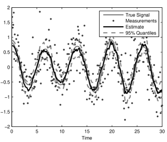
Figure 1: The result of applying continuous-discrete particle filter with EKF proposal to a simulated noisy pendulum data.

Figure 1 shows the result of applying the continuous-discrete particle filter with EKF proposal and $1000$ particles to a simulated data. The data was generated from the noisy pendulum model with process noise spectral density $q=0.01$, angular velocity $a=1$ and the sampling step size was $\Delta t=0.1$. The estimate can be seen to be quite close to the true signal.

In the simulation, the true measurement variance was $\sigma^{2}=0.25$. The prior distribution used for the unknown variance parameter was $\sigma^{2}\sim\text{Inv-}\chi^{2}(2,0.2)$.

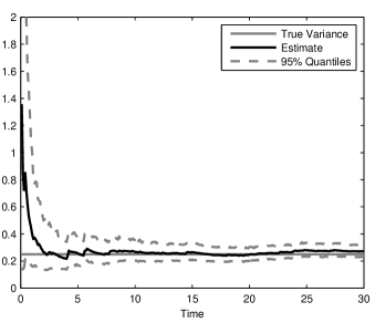
Figure 2: The evolution of variance distribution in the noisy pendulum problem.

The evolution of the posterior distribution of the variance parameter is shown in the Figure 2. In the beginning the uncertainty about the variance is higher, but the distribution quickly concentrates to the neighborhood of the true value.

3.2 Spread of Infectious Diseases

The classic model for the dynamics of infectious diseases is the SIR model (The model is called the SIR model, because the variables $X(t)$, $Y(t)$, and $Z(t)$ denote the susceptible, infective and removed compartments and for this reason are often denoted as $S(t)$, $I(t)$, and $R(t)$, respectively) (Kermack and McKendrick, 1927; Anderson and May, 1991; Murray, 1993; Hethcote, 2000), which is valid for sufficiently large $N$:

$$\mathrm{d}X/\mathrm{d}t =-b\,Y\,X/N,\qquad X(0) =X_{0},$$ (44)

$$\mathrm{d}Y/\mathrm{d}t =b\,Y\,X/N-g\,Y,\qquad Y(0) =Y_{0},$$ (45)

$$\mathrm{d}Z/\mathrm{d}t =g\,Y,\qquad Z(0) =Z_{0},$$ (46)

where $X(t)$ is the number of susceptibles at time $t$, $X_{0}\geq 0$ is the initial number of susceptibles, $Y(t)$ is the number of infectives who are capable of transmitting the infection, $Y_{0}\geq 0$ is the initial number of infectives, $Z(t)$ is the number of recovered or dead individuals which cannot be infected anymore, $Z_{0}\geq 0$ is the initial number of individuals in this class, $N=X(t)+Y(t)+Z(t)$ is the (constant) total number of individuals, $b$ is the contact rate which determines the rate of individuals moving from susceptible class to infectious class, and $g$ is the waiting time parameter such that $1/g$ is the average length of the infectious period.

If we model the contact number $\sigma=b/g$ as the exponential of the Brownian motion, then the stochastic equations for the proportions of individuals in each class can be written as (Särkkä, 2006b):

$$\begin{split}\mathrm{d}x/\mathrm{d}t&=-g\,\exp(\lambda)\,y\,x\\ \mathrm{d}y/\mathrm{d}t&=g\,\exp(\lambda)\,y\,x-g\,y\\ \mathrm{d}\lambda&=q^{1/2}\,\mathrm{d}\beta,\end{split}$$ (47)

where $\beta(t)$ is a standard Brownian motion and $\lambda=\ln\sigma$.

A suitable initial distribution for $x(0)$ and $y(0)$ is

$$y(0) \sim\mathrm{Beta}(\alpha_{y},\beta_{y}),$$ (48)

$$x(0) =1-y(0),$$ (49)

where $\beta_{y}\gg\alpha_{y}$. The initial conditions $z(0)$ can be assumed to be zero without loss of generality.

In the classical SIR model the values $X(t)$, $Y(t)$ and $Z(t)$ are not restricted to integer values, and thus they cannot be interpreted as counts as such. A sensible stochastic interpretation of these values is that they are the average numbers of individuals in each class and the actual numbers of individuals are Poisson distributed with these means.

Assume that the number of dead individuals is recorded. Then the number of the dead individuals $d_{k}$ on time period $[t_{k-1},t_{k}]$ has the distribution

$$p(d_{k}\,|\,\{x(\tau),y(\tau):0\leq\tau\leq t_{k}\},N)=\mathrm{Poisson}(d_{k}\,|\,N\,\theta_{k}),$$ (50)

where

$$\theta_{k}=x(t_{k-1})-x(t_{k})+y(t_{k-1})-y(t_{k}).$$ (51)

The population size $N$ is unknown and it can be modeled as having a Gamma prior distribution

$$p(N)=\mathrm{Gamma}(N\,|\,\alpha_{0},\beta_{0}),$$ (52)

with some suitably chosen $\alpha_{0}$ and $\beta_{0}$. As shown in (Särkkä, 2006b) this model is now of such form that it is possible to integrate out the population size $N$ from the equations and the Algorithm 2.4 can be applied.

The continuous-discrete SIR filter was applied to the classical Bombay plague data presented in (Kermack and McKendrick, 1927). An EKF based Gaussian process approximation was used as the importance process (see, Särkkä, 2006b, for details) and $10000$ particles was used. The prior distribution for proportion of initial infectives was $\text{Beta}(1,100)$. The population size prior was $\text{Gamma}(10,0.001)$. The waiting time parameter was assumed to be $g=1$. The prior distribution for $\lambda(0)$ was $\operatorname{N}(\ln(5),4)$. The diffusion coefficient of the Brownian motion was $q=0.001$.

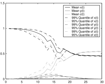
Figure 3: Filtered estimates of values of $x(t)$, $y(t)$, and $z(t)$ from the Bombay data.

The final filtered estimates of the histories of $x(t)$, $y(t)$, and $z(t)$ are shown in Figure 3. These estimates are filtered estimates, that is, they are conditional to the previously observed measurements only. That is, the estimate on week $t$ is the estimate that could be actually computed on week $t$ without any knowledge of the future observations. The estimates look quite much as what would be expected: the proportion of susceptibles $x(t)$ decreases in time and the number of infectives $y(t)$ increases up to a maximum and then decreases to zero. However, these estimated values are not very useful themselves. The reason for this is that, for example, the value $x_{\infty}$ which is the remaining value of susceptibles in the end depends on the choice of $g$ and other prior parameters. That is, these estimated values are not absolute in the sense that their values depend heavily on the prior assumptions.

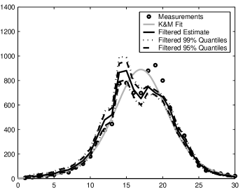
Figure 4: Filtered estimate of $\mathrm{d}Z/\mathrm{d}t$ from the Bombay data. The estimate of (Kermack and McKendrick, 1927) is also shown for comparison.

Much more informative quantity is the value $\mathrm{d}Z/\mathrm{d}t$, whose filtered estimate is shown in Figure 4. The classical estimate presented in (Kermack and McKendrick, 1927) is also shown. The SIR filter estimate can be seen to differ a bit from the classical estimate, but still both the estimates look quite much like what would be expected. Note that the classical estimate is based on all measurements, whereas the filtered estimate is based on observations made up to that time only. That is, the filter estimate could be actually computed on week $t$, but the classical estimate could not.

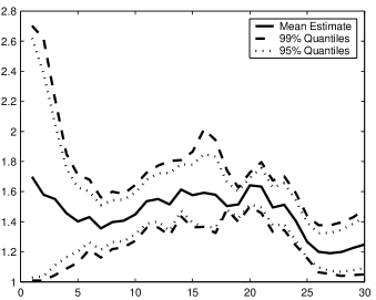
Figure 5: Bombay plague: Filtered estimate of value $\sigma(t)$.

The filtered estimates of values $\sigma(t)$ are shown in Figure 5. The value can be seen to vary a bit on time, but the estimated expected value remains on the range $[1.4,1.8]$ all the time. As can be seen from the figure, according to the data the value of $\sigma(t)$ is not constant. This is not surprising, because the spatial and other unknown effects are not accounted at all in the classical SIR model and these effects typically affect the number of contacts.

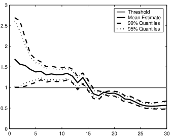
Figure 6: Bombay plague: Filtered estimate of value $x(t)\,\sigma(t)$.

A very useful indicator value is $\sigma(t)\,x(t)$, whose filtered estimate is shown in Figure 6. In the deterministic SIR model with constant $\sigma$ this indicator defines the asymptotic behavior of the epidemic (see, e.g., Hethcote, 2000): If $\sigma x(t)\leq 1$ then the number of infectives will decrease to zero as $t\rightarrow\infty$. If $\sigma x(t)>1$ then the number of infectives will first increase up to a maximum and then decrease to zero. As can be seen from the Figure 6 the filtered estimate of the indicator value goes below 1 just after the maximum somewhere between weeks 15–16, which can be seen in Figure 4. That is, the estimated value of $\sigma(t)\,x(t)$ could be used as an indicator, which tells if the epidemic is over or not.

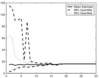
Figure 7: Bombay plague: Filtered estimate of time of maximum of epidemic.

Using the particles it is also possible to predict ahead to the future and estimate the time when the maximum of the epidemic will be reached. The estimate computed from the filtering result is shown in the Figure 7. Again, the estimates are filtered estimates and the estimate on week $t$ could be actually computed on week $t$, because it depends only on the counts observed up to that time. The filtered estimate can be seen to quickly converge to the values near the correct maximum on weeks 15–16. It is interesting to see that the prediction is quite accurate already around the week 10, which is far before reaching the actual maximum. If this kind of prediction had been done on, for example, week 10 of the disease, it would have predicted the time of actual epidemic maximum quite accurately. After the maximum has been observed, the estimate quickly converges to a constant value, which according to the Figure 4 is likely to be near the true maximum.

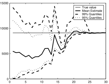
Figure 8: Bombay plague: Filtered estimated of number of deaths.

A very useful estimate is also the expected total number of deaths caused by the epidemic. This can be computed from the filtered estimates and the result is shown in Figure 8. In the beginning the estimate is very diffuse, but after maximum has been reached the estimate converges near the correct value. The estimate is a bit less than the observed value long before reaching the maximum, which might be due to existence of two maximums in the observed data (see, Figure 4). Because the second maximum is not predicted by the model, the extra number of deaths caused by it cannot be seen in the predictions.

4 Discussion

The importance processes used in the continuous-discrete particle filtering examples are very simple and better alternatives definitely exists. In principle, the optimal importance process in the continuous-discrete particle filtering case would have the same law as the smoothing solution. Thus, constructing the importance process based on the smoothing solution instead of linearly interpolated filtering solutions, as in this article, could lead to more efficient particle filtering methods. In some cases it could be possible to construct a process, which would have exactly the same law as the optimal importance process.

A weakness in the continuous-discrete particle filtering framework is that the importance process has to be scaled before sampling. In practice, this restricts the possible forms of importance processes to those having the same dispersion matrix as the original process. However, this a bit more general case with explicit scaling is treated here instead of requiring $\mathit{L}(t)=\mathit{B}(t)$, because this leaves more room to the possibility that maybe the equations could be modified such that the scaling of the importance process would not be needed.

Another weakness of the framework is that the time-discretization introduces biasedness to the estimation. The time-discretization is due to the usage of numerical integration methods for SDEs, which use discretization in time. However, there exists method for simulating SDEs without time-discretization (Beskos et al., 2006) and maybe by using this kind of methods this biasedness could be eliminated.

The continuous-discrete sequential importance resampling framework could be extended to the case of stochastic differential equations driven by more general martingales, for example, general Lévy processes such as compound Poisson processes (Applebaum, 2004). This would allow modeling of sudden changes in signals. This extension could be possible by simply replacing the Brownian motion in the Girsanov theorem by a more general martingale.

It could be possible to generalize the continuous-discrete sequential importance sampling framework to continuous-time filtering problems. Then the extended Kalman-Bucy filter or the unscented Kalman-Bucy filter (Särkkä, 2006b, 2007) could be used for forming the importance process and the actual filtering result would be formed by weighting the importance process samples properly.

The likelihood ratio expressions in Theorems A.3 and A.5 have an interesting connection to the variational method considered in article (Archambeau et al., 2007). If we select the processes as

$$\mathrm{d}\mathbf{x}(t) =\mathbf{f}(\mathbf{x}(t),t)\,\mathrm{d}t+\sqrt{\Sigma}\,\mathrm{d}\mathrm{\boldsymbol{\beta}}(t)$$ (53)

$$\mathrm{d}\mathbf{s}(t) =\mathbf{f}_{L}(\mathbf{s}(t),t)\,\mathrm{d}t+\sqrt{\Sigma}\,\mathrm{d}\mathrm{\boldsymbol{\beta}}(t),$$ (54)

where $\mathbf{x}(t)$ is a process with density $p(\cdot)$ and $\mathbf{s}(t)$ is a process with density $q(\cdot)$, then by taking the expectation of negative logarithm of (63) we get the expression for the KL-divergence between $q$ and $p$:

$$\begin{split}\mathrm{KL}[q\,|\,p]&=\operatorname{E}\Big{[}\frac{1}{2}\int_{0}^{t}\big{\{}\mathbf{f}(\mathbf{s}(t),t)-\mathbf{f}_{L}(\mathbf{s}(t),t)\big{\}}^{T}\Sigma^{-1}\big{\{}\mathbf{f}(\mathbf{s}(t),t)-\mathbf{f}_{L}(\mathbf{s}(t),t)\big{\}}\,\mathrm{d}t\Big{]},\end{split}$$ (55)

which is exactly the expression obtained heuristically in Archambeau et al. (2007). Thus the extensions to singular models would also apply to that method.

5 Conclusions

In this article, a new class of methods for continuous-discrete sequential importance sampling (particle filtering) has been presented. These methods are based on transformations of probability measures using the Girsanov theorem. The new methods are applicable to a general class of models. In particular, they can be applied to many models with singular dispersion matrices, unlike many previously proposed measure transformation based sampling methods. The new methods have been illustrated in a simulated problem, where both the implementation details of the algorithms and the simulation results have been reported. The methods have also been applied to estimation of the spread of an infectious disease based on counts of dead individuals.

The classical continuous-discrete extended Kalman filter as well as the recently developed continuous-discrete unscented Kalman filter can be used for forming importance processes for the new continuous-discrete particle filters. This way the efficiency of the Gaussian approximation based filters can be combined with the accuracy of the particle approximations. Closed form marginalization or Rao-Blackwellization can be applied if the model is conditionally Gaussian or if the model contains unknown static parameters and has a suitable conjugate form. In most cases Rao-Blackwellization leads to a significant improvement in the efficiency of the particle filtering algorithm.

Appendix A Likelihood Ratios of SDEs

In the computation of the likelihood ratios of stochastic differential equations we need a slightly generalized version of the Girsanov theorem (Kallianpur, 1980; Karatzas and Shreve, 1991; Øksendal, 2003). The generalized theorem can be obtained, for example, as a special case from the theorems presented in Delyon and Hu (2006).

Theorem A.1 (Girsanov)

Let $\mathrm{\boldsymbol{\beta}}=(\beta_{1},\ldots,\beta_{d})$ be a Brownian motion with diffusion matrix $\mathit{Q}(t)$ under the probability measure $\mathbb{P}$. Let $\mathrm{\boldsymbol{\theta}}:\Omega\times\mathbb{R}_{+}\mapsto\mathbb{R}^{d}$ be an adapted process such that the process $Z$ defined as

$$Z(t)=\exp\left\{\int_{0}^{t}\mathrm{\boldsymbol{\theta}}^{T}(t)\mathrm{d}\mathrm{\boldsymbol{\beta}}(t)-\frac{1}{2}\int_{0}^{t}\mathrm{\boldsymbol{\theta}}^{T}(t)\,\mathit{Q}(t)\,\mathrm{\boldsymbol{\theta}}(t)\mathrm{d}t\right\},$$ (56)

satisfies $\operatorname{E}[Z(t)]=1$. Then the process

$$\mathrm{d}\tilde{\mathrm{\boldsymbol{\beta}}}(t)=\mathrm{d}\mathrm{\boldsymbol{\beta}}(t)-\mathit{Q}(t)\,\mathrm{\boldsymbol{\theta}}(t)\mathrm{d}t$$ (57)

is a Brownian motion with diffusion matrix $\mathit{Q}(t)$ under the probability measure $\tilde{\mathbb{P}}$ defined via the relation

$$\operatorname{E}\left[\frac{\mathrm{d}\tilde{\mathbb{P}}}{\mathrm{d}\mathbb{P}}\,\bigg{|}\,\mathcal{F}_{t}\right]=Z(t),$$ (58)

where $\mathcal{F}_{t}$ is the natural filtration of the Brownian motion $\mathrm{\boldsymbol{\beta}}(t)$.

Proof A.2.

See, for example, Delyon and Hu (2006).

Theorem A.3 (Transformation of SDE Solutions I).

Let

$$\mathrm{d}\mathbf{x}(t) =\mathbf{f}(\mathbf{x}(t),t)\,\mathrm{d}t+\mathit{L}(t)\,\mathrm{d}\mathrm{\boldsymbol{\beta}}(t),\qquad\mathbf{x}(0)=x_{0}$$ (59)

$$\mathrm{d}\mathbf{s}(t) =\mathbf{g}(\mathbf{s}(t),t)\,\mathrm{d}t+\mathit{B}(t)\,\mathrm{d}\mathrm{\boldsymbol{\beta}}(t),\qquad\mathbf{s}(0)=x_{0},$$ (60)

where $\mathrm{\boldsymbol{\beta}}(t)$ is a Brownian motion with diffusion matrix $\mathit{Q}(t)$ with respect to measure $\mathbb{P}$. Let be its natural filtration. The matrices $\mathit{L}(t)$ and $\mathit{B}(t)$ are assumed to be invertible for all $t$. Now the process $\mathbf{s}^{*}(t)$ defined as

$$\mathrm{d}\mathbf{s}^{*}=\mathit{L}(t)\,\mathit{B}^{-1}(t)\,\mathrm{d}\mathbf{s},\qquad\mathbf{s}(0)=\mathbf{x}_{0}$$ (61)

is a weak solution to the Equation (59) under the measure $\tilde{\mathbb{P}}$ defined by the relation

$$\operatorname{E}\left[\frac{\mathrm{d}\tilde{\mathbb{P}}}{\mathrm{d}\mathbb{P}}\,\bigg{|}\,\right]=Z(t).$$ (62)

where

$$\begin{split}Z(t)&=\exp\Big{[}\int_{0}^{t}\big{\{}\mathbf{f}(\mathbf{s}^{*}(t),t)-\mathit{L}(t)\,\mathit{B}^{-1}(t)\,\mathbf{g}(\mathbf{s}(t),t)\big{\}}^{T}\,\mathit{L}^{-T}(t)\,\mathit{Q}^{-1}(t)\,\mathrm{d}\mathrm{\boldsymbol{\beta}}(t)\\ &\qquad-\frac{1}{2}\int_{0}^{t}\big{\{}\mathbf{f}(\mathbf{s}^{*}(t),t)-\mathit{L}(t)\,\mathit{B}^{-1}(t)\,\mathbf{g}(\mathbf{s}(t),t)\big{\}}^{T}\\ &\quad\qquad\times\big{\{}\mathit{L}(t)\,\mathit{Q}(t)\,\mathit{L}^{T}(t)\big{\}}^{-1}\big{\{}\mathbf{f}(\mathbf{s}^{*}(t),t)-\mathit{L}(t)\,\mathit{B}^{-1}(t)\,\mathbf{g}(\mathbf{s}(t),t)\big{\}}\,\mathrm{d}t\Big{]}\end{split}$$ (63)

Proof A.4.

By substituting the expression (60) into Equation (61), solving for $\mathrm{d}\mathrm{\boldsymbol{\beta}}(t)$, we get

$$\mathrm{d}\mathrm{\boldsymbol{\beta}}(t)=\mathit{L}^{-1}(t)\,\mathrm{d}\mathbf{s}^{*}-\mathit{B}^{-1}(t)\,\mathbf{g}(\mathbf{s}(t),t)\,\mathrm{d}t.$$ (64)

If we now define

$$\mathrm{\boldsymbol{\theta}}(t)=\mathit{Q}^{-1}(t)\,\mathit{L}^{-1}(t)\,\mathbf{f}(\mathbf{s}^{*}(t),t)-\mathit{Q}^{-1}(t)\,\mathit{B}^{-1}(t)\,\mathbf{g}(\mathbf{s}(t),t),$$ (65)

then under the measure $\tilde{\mathbb{P}}$ defined by (62) and (63) with the process $\mathrm{\boldsymbol{\theta}}(t)$ defined as above, the following process is a Brownian motion with diffusion matrix $\mathit{Q}(t)$:

$$\begin{split}\mathrm{d}\tilde{\mathrm{\boldsymbol{\beta}}}(t)&=\mathrm{d}\mathrm{\boldsymbol{\beta}}(t)-\mathit{Q}(t)\,\mathrm{\boldsymbol{\theta}}(t)\mathrm{d}t\\ &=\mathit{L}^{-1}(t)\,\mathrm{d}\mathbf{s}^{*}-\mathit{B}^{-1}(t)\,\mathbf{g}(\mathbf{s}(t),t)\,\mathrm{d}t\\ &-\mathit{Q}(t)\,\mathit{Q}^{-1}(t)\,\mathit{L}^{-1}(t)\,\mathbf{f}(\mathbf{s}^{*}(t),t)\,\mathrm{d}t+\mathit{Q}(t)\,\mathit{Q}^{-1}(t)\,\mathit{B}^{-1}(t)\,\mathbf{g}(\mathbf{s}(t),t)\,\mathrm{d}t\\ &=\mathit{L}^{-1}(t)\,\mathrm{d}\mathbf{s}^{*}-\mathit{L}^{-1}(t)\,\mathbf{f}(\mathbf{s}^{*}(t),t)\,\mathrm{d}t\end{split}$$ (66)

By rearranging we get that

$$\mathrm{d}\mathbf{s}^{*}=\mathbf{f}(\mathbf{s}^{*}(t),t)\,\mathrm{d}t+\mathit{L}(t)\,\mathrm{d}\tilde{\mathrm{\boldsymbol{\beta}}}(t)$$ (67)

and thus the result follows. The explicit expression for the likelihood ratio is given as follows:

$$\begin{split}Z(t)&=\exp\Big{[}\int_{0}^{t}\big{\{}\mathit{Q}^{-1}(t)\,\mathit{L}^{-1}(t)\,\mathbf{f}(\mathbf{s}^{*}(t),t)-\mathit{Q}^{-1}(t)\,\mathit{B}^{-1}(t)\,\mathbf{g}(\mathbf{s}(t),t)\big{\}}^{T}\,\mathrm{d}\mathrm{\boldsymbol{\beta}}(t)\\ &-\frac{1}{2}\int_{0}^{t}\big{\{}\mathit{Q}^{-1}(t)\,\mathit{L}^{-1}(t)\,\mathbf{f}(\mathbf{s}^{*}(t),t)-\mathit{Q}^{-1}(t)\,\mathit{B}^{-1}(t)\,\mathbf{g}(\mathbf{s}(t),t)\big{\}}^{T}\\ &\times\mathit{Q}(t)\big{\{}\mathit{Q}^{-1}(t)\,\mathit{L}^{-1}(t)\,\mathbf{f}(\mathbf{s}^{*}(t),t)-\mathit{Q}^{-1}(t)\,\mathit{B}^{-1}(t)\,\mathbf{g}(\mathbf{s}(t),t)\big{\}}\,\mathrm{d}t\Big{]}\\ &=\exp\Big{[}\int_{0}^{t}\big{\{}\mathbf{f}(\mathbf{s}^{*}(t),t)-\mathit{L}(t)\,\mathit{B}^{-1}(t)\,\mathbf{g}(\mathbf{s}(t),t)\big{\}}^{T}\,\mathit{L}^{-T}(t)\,\mathit{Q}^{-1}(t)\,\mathrm{d}\mathrm{\boldsymbol{\beta}}(t)\\ &\qquad-\frac{1}{2}\int_{0}^{t}\big{\{}\mathit{L}^{-1}(t)\,\mathbf{f}(\mathbf{s}^{*}(t),t)-\mathit{L}(t)\,\mathit{B}^{-1}(t)\,\mathbf{g}(\mathbf{s}(t),t)\big{\}}^{T}\\ &\quad\qquad\times\big{\{}\mathit{L}^{-T}(t)\,\mathit{Q}^{-1}(t)\,\mathit{Q}(t)\mathit{Q}(t)^{-1}\,\mathit{L}^{-1}(t)\big{\}}\\ &\quad\qquad\times\big{\{}\mathbf{f}(\mathbf{s}^{*}(t),t)-\mathit{L}(t)\,\mathit{B}^{-1}(t)\,\mathbf{g}(\mathbf{s}(t),t)\big{\}}\,\mathrm{d}t\Big{]}\\ &=\exp\Big{[}\int_{0}^{t}\big{\{}\mathbf{f}(\mathbf{s}^{*}(t),t)-\mathit{L}(t)\,\mathit{B}^{-1}(t)\,\mathbf{g}(\mathbf{s}(t),t)\big{\}}^{T}\,\mathit{L}^{-T}(t)\,\mathit{Q}^{-1}(t)\,\mathrm{d}\mathrm{\boldsymbol{\beta}}(t)\\ &\qquad-\frac{1}{2}\int_{0}^{t}\big{\{}\mathbf{f}(\mathbf{s}^{*}(t),t)-\mathit{L}(t)\,\mathit{B}^{-1}(t)\,\mathbf{g}(\mathbf{s}(t),t)\big{\}}^{T}\\ &\quad\qquad\times\big{\{}\mathit{L}(t)\,\mathit{Q}(t)\,\mathit{L}^{T}(t)\big{\}}^{-1}\big{\{}\mathbf{f}(\mathbf{s}^{*}(t),t)-\mathit{L}(t)\,\mathit{B}^{-1}(t)\,\mathbf{g}(\mathbf{s}(t),t)\big{\}}\,\mathrm{d}t\Big{]}\end{split}$$ (68)

Theorem A.5 (Transformation of SDE Solutions II).

Assume that processes $\mathbf{x}_{1}(t)$, $\mathbf{x}_{2}(t)$, $\mathbf{s}_{1}(t)$ and $\mathbf{s}_{2}(t)$ are generated by the stochastic differential equations

$$\frac{\mathrm{d}\mathbf{x}_{1}}{\mathrm{d}t} =\mathbf{f}_{1}(\mathbf{x}_{1},\mathbf{x}_{2},t),\qquad \mathbf{x}_{1}(0)=\mathbf{x}_{1,0}$$ (69)

$$\mathrm{d}\mathbf{x}_{2} =\mathbf{f}_{2}(\mathbf{x}_{1},\mathbf{x}_{2},t)\,\mathrm{d}t+\mathit{L}(t)\,\mathrm{d}\mathrm{\boldsymbol{\beta}},\qquad \mathbf{x}_{2}(0)=\mathbf{x}_{2,0}$$ (70)

$$\frac{\mathrm{d}\mathbf{s}_{1}}{\mathrm{d}t} =\mathbf{f}_{1}(\mathbf{s}_{1},\mathbf{s}_{2},t),\qquad \mathbf{s}_{1}(0)=\mathbf{x}_{1,0}$$ (71)

$$\mathrm{d}\mathbf{s}_{2} =\mathbf{g}_{2}(\mathbf{s}_{1},\mathbf{s}_{2},t)\,\mathrm{d}t+\mathit{B}(t)\,\mathrm{d}\mathrm{\boldsymbol{\beta}},\qquad \mathbf{s}_{2}(0)=\mathbf{x}_{2,0},$$ (72)

where $\mathit{L}(t)$ and $\mathit{B}(t)$ are invertible matrices for all $t\geq 0$ and under the measure $\mathbb{P}$, $\mathrm{\boldsymbol{\beta}}(t)$ is a Brownian motion with diffusion matrix $\mathit{Q}(t)$. Then the processes $\mathbf{s}_{1}$ and $\mathbf{s}_{2}$ defined as

$$\frac{\mathrm{d}\mathbf{s}^{*}_{1}}{\mathrm{d}t} =\mathbf{f}_{1}(\mathbf{s}^{*}_{1},\mathbf{s}^{*}_{2},t),\qquad \mathbf{s}^{*}_{1}(0)=\mathbf{x}_{1,0}$$ (73)

$$\mathrm{d}\mathbf{s}^{*}_{2} =\mathit{L}(t)\,\mathit{B}^{-1}(t)\,\mathrm{d}s_{2},\qquad \mathbf{s}^{*}_{2}(0)=\mathbf{x}_{2,0}$$ (74)

are weak solutions to the Equations (69) and (70) under the measure $\tilde{\mathbb{P}}$ defined by the relation

$$\operatorname{E}\left[\frac{\mathrm{d}\tilde{\mathbb{P}}}{\mathrm{d}\mathbb{P}}\,\bigg{|}\,\right]=Z(t).$$ (75)

where

$$\begin{split}Z(t)&=\exp\Big{[}\int_{0}^{t}\big{\{}\mathbf{f}_{2}(\mathbf{s}^{*}_{1}(t),\mathbf{s}^{*}_{2}(t),t)-\mathit{L}(t)\,\mathit{B}^{-1}(t)\,\mathbf{g}_{2}(\mathbf{s}_{1}(t),\mathbf{s}_{2}(t),t)\big{\}}^{T}\\ &\qquad\qquad\times\mathit{L}^{-T}(t)\,\mathit{Q}^{-1}(t)\,\mathrm{d}\mathrm{\boldsymbol{\beta}}(t)\\ &\qquad-\frac{1}{2}\int_{0}^{t}\big{\{}\mathbf{f}_{2}(\mathbf{s}^{*}_{1}(t),\mathbf{s}^{*}_{2}(t),t)-\mathit{L}(t)\,\mathit{B}^{-1}(t)\,\mathbf{g}_{2}(\mathbf{s}_{1}(t),\mathbf{s}_{2}(t),t)\big{\}}^{T}\\ &\qquad\qquad\times\big{\{}\mathit{L}^{T}(t)\,\mathit{Q}(t)\,\mathit{L}(t)\big{\}}^{-1}\\ &\qquad\qquad\times\big{\{}\mathbf{f}_{2}(\mathbf{s}^{*}_{1}(t),\mathbf{s}^{*}_{2}(t),t)-\mathit{L}(t)\,\mathit{B}^{-1}(t)\,\mathbf{g}_{2}(\mathbf{s}_{1}(t),\mathbf{s}_{2}(t),t)\big{\}}\,\mathrm{d}t\Big{]}\end{split}$$ (76)

Proof A.6.

From equations (71), (72), (73) and (74) we get that

$$\mathrm{d}\mathrm{\boldsymbol{\beta}}(t)=\mathit{L}^{-1}(t)\,\mathrm{d}\mathbf{s}^{*}_{2}-\mathit{B}^{-1}(t)\,\mathbf{g}_{2}(\mathbf{s}_{1}(t),\mathbf{s}_{2}(t),t)\,\mathrm{d}t.$$ (77)

If we now define

$$\mathrm{\boldsymbol{\theta}}(t)=\mathit{Q}^{-1}(t)\,\mathit{L}^{-1}(t)\,\mathbf{f}_{2}(\mathbf{s}^{*}_{1}(t),\mathbf{s}^{*}_{2}(t),t)-\mathit{Q}^{-1}(t)\,\mathit{B}^{-1}(t)\,\mathbf{g}_{2}(\mathbf{s}_{1}(t),\mathbf{s}_{2}(t),t),$$ (78)

then similarly as in proof of Theorem A.3, we get that the process $\tilde{\mathrm{\boldsymbol{\beta}}}(t)$ defined as

$$\begin{split}\mathrm{d}\tilde{\mathrm{\boldsymbol{\beta}}}(t)&=\mathrm{d}\mathrm{\boldsymbol{\beta}}(t)-\mathit{Q}(t)\,\mathrm{\boldsymbol{\theta}}(t)\mathrm{d}t\\ &=\mathit{L}^{-1}(t)\,\mathrm{d}\mathbf{s}^{*}_{2}-\mathit{B}^{-1}(t)\,\mathbf{g}_{2}(\mathbf{s}_{1}(t),\mathbf{s}_{2}(t),t)\,\mathrm{d}t\\ &\quad-\mathit{Q}(t)\,\mathit{Q}^{-1}(t)\,\mathit{L}^{-1}(t)\,\mathbf{f}_{2}(\mathbf{s}^{*}_{1}(t),\mathbf{s}^{*}_{2}(t),t)\,\mathrm{d}t\\ &\quad+\mathit{Q}(t)\,\mathit{Q}^{-1}(t)\,\mathit{B}^{-1}(t)\,\mathbf{g}_{2}(\mathbf{s}_{1}(t),\mathbf{s}_{2}(t),t)\,\mathrm{d}t\\ &=\mathit{L}^{-1}(t)\,\mathrm{d}\mathbf{s}^{*}_{2}-\mathit{L}^{-1}(t)\,\mathbf{f}_{2}(\mathbf{s}^{*}_{1}(t),\mathbf{s}^{*}_{2}(t),t)\,\mathrm{d}t\end{split}$$ (79)

is a Brownian motion with respect to measure $\tilde{\mathbb{P}}$ and thus $\mathbf{s}^{*}_{1}$ and $\mathbf{s}^{*}_{2}$ are the weak solutions to the equations (69) and (70).

Appendix B Acknowledgment

The author would like to thank Aki Vehtari, Jouko Lampinen and Ilkka Kalliomäki for helpful discussions and comments on the manuscript.

References

- Alonso and Finn (1980) Alonso, M. and E. J. Finn (1980). Fundamental University Physics, Volume I: Mechanics and Thermodynamics (2nd ed.). Addison-Wesley.
- Anderson and May (1991) Anderson, R. M. and R. M. May (1991). Infectious Diseases of Humans: Dynamics and Control. Oxford University Press.
- Applebaum (2004) Applebaum, D. (2004). Lévy Processes and Stochastic Calculus. Cambridge University Press.
- Archambeau et al. (2007) Archambeau, C., D. Cornford, M. Opper, and J. Shawe-Taylor (2007). Gaussian process approximations of stochastic differential equations. Journal of Machine Learning Research Workshop and Conference Proceedings 1, 1–16.
- Bar-Shalom et al. (2001) Bar-Shalom, Y., X.-R. Li, and T. Kirubarajan (2001). Estimation with Applications to Tracking and Navigation. Wiley Interscience.
- Beskos et al. (2006) Beskos, A., O. Papaspiliopoulos, G. Roberts, and P. Fearnhead (2006). Exact and computationally efficient likelihood-based estimation for discretely observed diffusion processes (with discussion). Journal of the Royal Statistical Society, Series B 68(3), 333 – 382.
- Chib et al. (2004) Chib, S., M. K. Pitt, and N. Shephard (2004). Likelihood based inference for diffusion driven models. Volume W20.
- Crisan (2003) Crisan, D. (2003). Exact rates of convergence for a branching particle approximation to the solution of the Zakai equation. Ann. Probab. 31(2), 693–718.
- Crisan et al. (1998) Crisan, D., J. Gaines, and T. Lyons (1998, October). Convergence of a branching particle method to the solution of the zakai equation. SIAM Journal on Applied Mathematics 58(5), 1568–1590.
- Crisan and Lyons (1999) Crisan, D. and T. Lyons (1999). A particle approximation of the solution of the Kushner-Stratonovitch equation. Probab. Theory Relat. Fields 115, 549–578.
- Delyon and Hu (2006) Delyon, B. and Y. Hu (2006). Simulation of conditioned diffusion and application to parameter estimation. Stochastic Processes and their Applications 116, 1660–1675.
- Doucet et al. (2001) Doucet, A., N. de Freitas, and N. Gordon (2001). Sequential Monte Carlo Methods in Practice. Springer.