Nonlinear Coherent Destruction of Tunneling

Abstract

We study theoretically two coupled periodically-curved optical waveguides with Kerr nonlinearity. We find that the tunneling between the waveguides can be suppressed in a wide range of parameters due to nonlinearity. Such suppression of tunneling is different from the coherent destruction of tunneling in a linear medium, which occurs only at the isolated degeneracy point of the quasienergies. We call this novel suppression nonlinear coherent destruction of tunneling. This nonlinear phenomenon can be observed readily with current experimental capability; it may also be observable in a different physical system, Bose-Einstein condensate.

Periodic driving force is an important and effective tool for coherently controlling quantum tunneling. This has been well demonstrated with a paradigmatic model, a free particle in a double-well potential and driven by a periodic external fieldP.Hanggi . With appropriately tuned parameters, the periodic driving force is able not only to enhance tunnelingLin -Vorobeichik1 but also to completely suppress itGrossmann -Steinberg . The latter is rather surprising and was discovered first by Grossmann et alGrossmann . It is now known as coherent destruction of tunneling (CDT)Grossmann . When it occurs, a localized wave packet prepared in one well remains in the same well and does not tunnel to the other well. In a periodically driven system, there are Floquet states and associated quasienergiesshirley . The CDT is found to occur only at the isolated degeneracy point of the quasienergiesGrossmann ; Grossmann2 .

Recently, this quantum phenomenon of CDT was observed experimentally with two coupled periodically-curved waveguidesLonghi2 (see Fig.1). In this classical optical system, the Maxwellian wave mimics the quantum wave while the periodic driving force is achieved by bending the waveguides periodically. Such a waveguide system is an ideal laboratory system for demonstrating the coherent control of quantum tunneling by periodic driving force. For example, tunneling enhancement has recently also been reported with two optical waveguidesVorobeichik .

In this Letter we consider a similar coupled waveguide system but with Kerr nonlinearity. With a well-known two-mode approximation, the system can be described by a two-mode nonlinear model with an external periodic driving force. This driving is characterized by two parameters, its frequency $w$ (the inverse of the period of the curved waveguide) and its strength $S$ (the curving magnitude of the waveguides) of the driving force. By numerically solving this two-mode nonlinear model, we find that the suppression of tunneling between the two coupled waveguides happens for a wide range of ratio $S/w$. This is in stark contrast to the CDT in curved linear waveguides that occurs at an isolated point of $S/w$, where the quasienergies of the system are degenerate. This extension of tunneling suppression region is caused by nonlinearity. Therefore, we call it nonlinear coherent destruction of tunneling (NCDT). We find that the range of ratio $S/w$ for NCDT increases steeply with nonlinear strength. The Floquet states and the quasienergies of this nonlinear model are also studied. We discover that there can be more than two Floquet states and quasienergies in a certain range of ratio $S/w$. These additional Floquet states form a triangle in the quasienergy levels. Our study reveals that these additional Floquet states are closely related to the NCDT.

The current experimental capability with nonlinear waveguides is examined. We find that the observation of NCDT is well within the current experimental ability. Note that the nonlinear two-mode model that we derived for the waveguides can also be used to describe the dynamics of a Bose-Einstein condensate in a double-well potential under a periodic modulationwang . This indicates that NCDT may also be observable with Bose-Einstein condensates.

Figure 1: Schematic drawing (not to scale) of two periodically curved optical waveguides placed parallel to each other.

In a weakly guiding dielectric structure, the effective two-dimensional wave equation for light propagation in nonlinear directional waveguides readsMicallef

$$i\frac{\lambda}{2\pi}\frac{\partial\psi}{\partial z}=-\frac{\lambda^{2}}{8\pi^{2}n_{s}}\frac{\partial^{2}\psi}{\partial x^{2}}+V[x-x_{0}(z)]\psi-|\psi|^{2}\psi.$$ (1)

where $\lambda$ is the free space wavelength of the light, $x_{0}(z)=A\cos(2\pi z/\Lambda)$, and $V(x)\equiv[n_{s}^{2}-n^{2}(x)]/(2n_{s})\simeq n_{s}-n(x)$, where $n(x)$ and $n_{s}$ are, respectively, the effective refractive index profile of the waveguides and the substrate refractive index. For the coupled waveguides as in Fig.1, $n(x)$ thus $V(x)$ have a double-well structure. The scalar electric field is related to $\psi$ through $E(x,z,t)=(1/2)(|n_{2}|n_{s}\epsilon_{0}c_{0}/2)^{-1/2}[\psi(x,z)\exp(-i\omega t+ikn_{s}z)+c.c.]$, where $n_{2}$ is the nonlinear refractive index of the medium, $k=2\pi/\lambda$, $\omega=kc_{0}$, and $c_{0}$ and $\epsilon_{0}$ are the speed of light and the dielectric constant in vacuum, respectively. The field normalization is taken such that $|\psi|^{2}/|n_{2}|$ gives the light intensity $I$ (in $W/m^{2}$). By means of a Kramers-Henneberger transformationkh $x^{\prime}=x-x_{0}(z),z^{\prime}=z$, and $\phi(x^{\prime},z^{\prime})=\psi(x^{\prime},z^{\prime})\exp[-i(2n_{s}\pi/\lambda)\dot{x}_{0}(z^{\prime})x^{\prime}-i(n_{s}\pi/\lambda)\int_{0}^{z^{\prime}}d\xi\dot{x}_{0}^{2}(\xi)]$ (the dot indicates the derivative with respect to $z^{\prime}$), Eq.(1) is then transformed to

$$i\frac{\lambda}{2\pi}\frac{\partial\phi}{\partial z^{\prime}} = -\frac{\lambda^{2}}{8\pi n_{s}}\frac{\partial^{2}\phi}{\partial x^{\prime 2}}+V(x^{\prime})\phi-|\phi|^{2}\phi+x^{\prime}F(z^{\prime})\phi$$ (2)

$$\equiv H_{0}\phi-|\phi|^{2}\phi+x^{\prime}F(z^{\prime})\phi.$$

where $F(z^{\prime})=n_{s}\ddot{x}_{0}(z^{\prime})=(4\pi^{2}An_{s}/\Lambda^{2})\cos(2\pi z^{\prime}/\Lambda)$ is the force induced by waveguide bending. It is clear that if we view $z$ (or $z^{\prime}$) as time $t$, the above equations can be regarded as describing the system of a nonlinear quantum wave in a double-well potential and under a periodic modulation.

We assume that the light in each waveguide of the coupler is single moded and neglect excitation of radiation modes. With a standard two-mode approximationLonghi3 ; khomeriki ; Jensen , we write

$$\phi(x^{\prime},z^{\prime})=e^{-\frac{2i\pi}{\lambda}E_{0}z^{\prime}}\Big{[}c_{1}(z^{\prime})u_{1}(x^{\prime})+c_{2}(z^{\prime})u_{2}(x^{\prime})\Big{]}\,,$$ (3)

where $u_{1}$ and $u_{2}$ are localized waves in two waveguides while the two coefficients are normalized to one, $|c_{1}|^{2}+|c_{2}|^{2}=1$. $E_{0}$ is defined as $E_{0}=\int u_{1,2}^{*}H_{0}u_{1,2}dx^{\prime}$. It is reasonable to assume that the localized wave is a Gaussian, $u_{1,2}(x^{\prime})=\sqrt{D}\exp[-(x^{\prime}\pm a/2)^{2}/2b^{2}]$, where $a$ is the distance between the two waveguides, $b$ is the half-width of each waveguide, and $D$ is related to the input power of the system $P(0)$ as $D=n_{2}P(0)/(\sqrt{\pi}b)$. $P(0)$ has the unit of $W/m$. The two-mode approximation eventually simplifies Eq.(2) to

$$i\dot{c_{1}} = \frac{v}{2}c_{2}-\frac{S}{2}\cos(wz^{\prime})c_{1}-\chi|c_{1}|^{2}c_{1},$$ (4)

$$i\dot{c_{2}} = \frac{v}{2}c_{1}+\frac{S}{2}\cos(wz^{\prime})c_{2}-\chi|c_{2}|^{2}c_{2},$$ (5)

where we have set $S=8\pi^{3}aAn_{s}/\Lambda^{2}\lambda$, $v=4\pi(\int u_{1}^{*}H_{0}u_{2}dx)/\lambda$, the modulation frequency $w=2\pi/\Lambda$, and $\chi=\sqrt{2\pi}n_{2}P(0)/(\lambda b)$ is an effective nonlinear coefficient. When $S=0$, Eqs. (4), (5) will be reduced to the well-known Jensen equationJensen . Note that $P(0)$ has the unit of $W/m$ is because the waveguide is two dimensional in our theoretical model. In experiments, $P(0)$ has the unit of $W$ and the waveguides are three dimensional. As a result, to relate our nonlinear parameter to the real experimental parameters, we choose $\chi=2\pi n_{2}P(0)/(\lambda\sigma_{\rm eff})$, where $\sigma_{\rm eff}$ is the effective cross-section of the waveguide, according to Ref.Eisenberg .

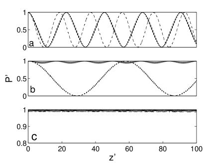
Figure 2: The intensity of light in the initially populated waveguide for the case of $\chi=0$ (dashed lines) and $\chi/v=0.4$(solid lines) with (a)$S/w=1.8$, (b)$S/w=2.2$, (c)$S/w=2.4$. Distance $z^{\prime}$ is in units of $1/v$. $w/v=10$.

To investigate tunneling effect, we solve the two nonlinear equations (4) and (5) numerically with the light initially localized in one of the two waveguides. With the numerical solution, we compute the intensity of the light staying in the initial well with $P^{\prime}(z^{\prime})=|c_{1}^{*}(0)c_{1}(z^{\prime})+c_{2}^{*}(0)c_{2}(z^{\prime})|^{2}$. Three sets of our results are shown in Fig.2(a,b,c). In the first set for $S/w=1.8$, we see that $P^{\prime}(z^{\prime})$ oscillates between zero and one for both linear case $\chi=0$ and nonlinear case $\chi/v=0.4$, demonstrating no suppression of tunneling. In the second set for $S/w=2.2$, we see a different scenario, the oscillation of $P^{\prime}(z^{\prime})$ is limited between $\sim$0.8 and one for the nonlinear case, showing suppression of tunneling, while there is no suppression for the linear case. In the third set for $S/w=2.4$, suppression of tunneling is seen for both linear and nonlinear cases. Such suppression of tunneling for the linear case is known as coherent destruction of tunnelingGrossmann . These numerical results demonstrate that nonlinearity can extend the parameter range of the suppression of tunneling. We call this new phenomenon nonlinear coherent destruction of tunneling (NCDT).

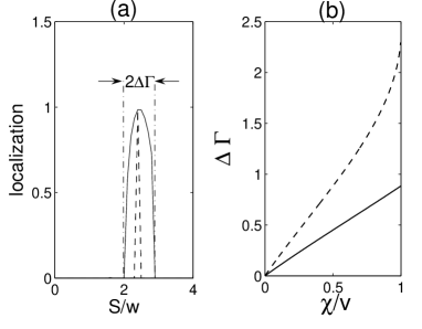
Figure 3: (a)Localization as a function of $S/w$. The solid line is for the nonlinear case $\chi/v=0.4$ and the dashed line is for the linear case $\chi=0$. $w/v=10$. (b) The width $\Delta\Gamma$ of the peak in (a) as a function of nonlinearity strength $\chi/v$ (solid line). The dashed line is for the width of the quasienergy triangle in Fig.4.

The extension of tunneling suppression regime of ratio $S/w$ by nonlinearity is more clearly demonstrated in Fig.3(a). In this figure, we have used localization, which is defined as the minimum value of $P^{\prime}(z^{\prime})$, to measure the suppress of tunneling. When there is large suppression of tunneling, localization is close to one; when there is no suppression,localization is zero. As clearly seen in Fig.3(a), the peak of localization (solid line) for $\chi/v=0.4$ is much wider than the peak for $\chi/v=0.0$ (dashed line). In Fig.3(b), we see the width of localization $\Delta\Gamma$ increases almost linearly with nonlinearity $\chi$(solid line). Note that, analytically, CDT occurs only at isolated points. That it has a narrow range in Fig.3(a) is because the evolution time is finite in numerical simulation.

As is well known, the CDT is connected to the degeneracy point of quasienergies in the systemGrossmann . Although our system is nonlinear, one can similarly define its Floquet state and quasienergy. That is, Eqs.(4,5) have solutions in the form of $\{c_{1},c_{2}\}=e^{-i\varepsilon z^{\prime}}\{\tilde{c}_{1}(z^{\prime}),\tilde{c}_{2}(z^{\prime})\}$, where both $\tilde{c}_{1}$ and $\tilde{c}_{2}$ are periodic with period of $\Lambda$. These Floquet states and corresponding quasienergies $\varepsilon$ can be found numerically. We first expand the periodic functions $\tilde{c}_{1,2}$ in terms of Fourier series with a cutoff. After plugging them into Eqs.(4,5), we obtain a set of nonlinear equations for the Fourier coefficients. By solving these equations numerically, we obtain the Floquet states and corresponding quasienergies $\varepsilon$. The results are plotted in Fig.4, where we witness a striking difference between the linear and nonlinear cases. As seen in Fig.4(a), for the linear case, there are two Floquet states for a given value of $S/w$ and there is only one isolated degeneracy point. For the nonlinear case, we notice that there are four Floquet states and three quasienergies in a certain range of $S/w$ with two of the Floquet states degenerate. The three quasienergies form a triangle in the quasienergy levels as seen in Fig.4(b,c). Our numerical computation shows that the width of the quasienergy triangle increases with nonlinearity $\chi$ as shown in Fig.3 (dashed line). As this increasing trend is similar to the localization width $\Delta\Gamma$, this offers us the first glimpse of link between NCDT and the quasienergies. Since the right corner of the triangle can be open, we define the width of the quasienergy triangle as the horizontal distance between the left corner and the upper corner.

Figure 4: Quasienergies at (a) $\chi=0$;(b) $\chi/v=0.4$; (c) $\chi/v=0.8$. Solid lines are for numerical results obtained with Eqs.(4,5) and circles for the approximation results for high frequencies with Eqs.(7,8). $w/v=3$.

A firm link between the NCDT and the triangle structure in the quasienergies can be established by looking into the Floquet states. We focus on the Floquet states that correspond to the lowest quasienergies in Fig.4. To measure how the Floquet state is localized in one of the two waveguides, we define $\langle|c_{1}|^{2}\rangle=(\int_{0}^{\Lambda}dz^{\prime}|c_{1}|^{2})/\Lambda$ for a given Floquet state $\{c_{1},c_{2}\}$. We have plotted this value for the lowest Floquet states in Fig.5. In this figure, we see clearly that only the Floquet states on the quasienergy triangle are localized. This thus demonstrates a clear link between the quasi-energy triangle and the NCDT. That there are two lines in Fig.5 reflects the fact that there is a two-fold degeneracy for the lowest quasienergies on the triangle.

Figure 5: Intensity in the first well for every Floquet state in the lowest quasienergy level at $\chi/v=0.4$, $w/v=3$.

The triangular structure in the quasienergy is very similar to the energy loop discovered within the context of nonlinear Landau-Zener tunnelingnlz . In fact, they are mathematically related. For high frequencies, $w\gg\max\{v,\chi\}$, which is usually the case for current experiments with optical waveguides, we take advantage of the transformation

$$\begin{array}[]{lll}c_{1}&=&c_{1}^{\prime}\exp[iS\sin(wz^{\prime})/2w],\cr\cr c_{2}&=&c_{2}^{\prime}\exp[-iS\sin(wz^{\prime})/2w].\end{array}$$ (6)

After averaging out the high frequency termswang , we find a non-driving nonlinear model,

$$i\dot{c_{1}^{\prime}} = \frac{v}{2}J_{0}(S/w)c_{2}^{\prime}-\chi|c_{1}^{\prime}|^{2}c_{1}^{\prime},$$ (7)

$$i\dot{c_{2}^{\prime}} = \frac{v}{2}J_{0}(S/w)c_{1}^{\prime}-\chi|c_{2}^{\prime}|^{2}c_{2}^{\prime},$$ (8)

where $J_{0}$ is the zeroth-order Bessel function. It is clear from the transformation in Eq.(6) that the eigenstates of the above time-independent nonlinear equations correspond to the Floquet states of Eqs.(4,5). We have computed the eigenstates of Eqs.(7,8) and the corresponding eigenenergies, which are plotted as circles in Fig.4. The consistency with the previous results is obvious. As is known in Ref.nlz , the above nonlinear model admits additional eigenstates when $\chi>J_{0}(S/w)v$. Therefore, this can be regarded as the condition for the extra Floquet states to appear for the driving nonlinear model Eqs.(4,5) at high frequencies.

So far, we have focused on self-focusing materials. Our approach and results will be very similar if one considers instead self-defocusing materials, for which the sign before the nonlinear term in Eq.(1) should be plus. Nonlinear coherent destruction of tunneling still occurs and the triangular structure also appears in the quasienergy levels but its direction is reversed as compared to the self-focusing case.

At present the nonlinear waveguides are readily available in labsEisenberg ; Al-hemyari ; Friberg . We take the experimental parameters in Ref.Al-hemyari to estimate our theoretical values in Eqs.(4,5). The wavelength of the laser light is $\lambda=1.55\mu$m, the effective cross-sectional area of the waveguide is $\sigma_{\rm eff}=12\mu$m², the nonlinear index $n_{2}=1.2\times 10^{-13}{\rm cm}^{2}/W$, and the shortest length for the light transfer from one waveguide to the other waveguide in the weak nonlinearity limit is $L_{c}\approx 2$cm. With the power input in the waveguides $P(0)\sim 100W$, we have

$$\frac{\chi}{v}=\frac{2\pi n_{2}P(0)L_{c}}{\pi\lambda\sigma_{\rm eff}}\approx 2\,.$$ (9)

This shows that strong nonlinear waveguides are available at optical labs and nonlinear coherent destruction of tunneling can be visualized in an optical experiment similar to the one in Ref.Longhi2 . We also want to mention briefly that NCDT may be applied to improve optical switching devicesAl-hemyari ; Friberg . The details will be discussed elsewhere.

In conclusion, we have studied the light propagation in a nonlinear periodically-curved waveguide directional coupler. We have found a new type of suppression of tunneling in this system, which is induced by nonlinearity and has no linear counterpart. We call it nonlinear coherent destruction of tunneling (NCDT) in analogy to a similar but different phenomenon in linear driving systems, coherent destruction of tunneling. The NCDT occurs for an extended range of ratio $S/w$, where $S$ is the strength of the driving and $w$ is its frequency. We have also found that the NCDT is closely related to a triangular structure appeared in the quasienergy levels of the nonlinear system. We have also pointed out that observation of the novel nonlinear phenomenon is well within the capacity of current experiments.

This work is supported by NSF of China (10504040), the 973 project of China(2005CB724500,2006CB921400), and the “BaiRen” program of Chinese Academy of Sciences.

References

- (1) M. Grifoni, and P.Hänggi, Phys. Rep. 304, 229(1998).
- (2) W. A. Lin and L. E. Ballentine, Phys. Rev. Lett. 65, 2927 (1990).
- (3) A. Peres, Phys. Rev. Lett. 67, 158 (1991).
- (4) I. Vorobeichik and N. Moiseyev, Phys. Rev. A, 59, 2511 (1999).
- (5) F. Grossmann, T. Dittrich, P. Jung, and P. Hanggi, Phys. Rev. Lett. 67, 516 (1991); Z. Phys. B 84, 315 (1991).
- (6) F. Grossmann and P. Hanggi, Europhys. Lett. 18, 571 (1992).
- (7) R. Bavli and H. Metiu, Phys. Rev. Lett. 69, 1986 (1992).
- (8) M. Steinberg and U. Peskin, J. Appl. Phys. 85, 270 (1999).
- (9) J. H. Shirley, Phys. Rev. 138, B979 (1965).
- (10) G. Della Valle, M. Ornigotti, E. Cianci, V. Foglietti, P. Laporta, and S. Longhi. e-print arXiv: quant-ph/0701121.
- (11) I. Vorobeichik, E. Narevicius, G. Rosenblum, M. Orenstein, and N. Moiseyev, Phys. Rev. Lett. 90, 176806 (2003).
- (12) Guan-Fang Wang, Li-Bin Fu and Jie Liu, Phys. Rev. A 73, 013619(2006).
- (13) R. W. Micallef, Y. S. Kivshar, J. D. Love, D. Burak, and R. Binder, Opt. Quantum Electron. 30, 751 (1998).
- (14) W.C. Henneberger, Phys. Rev. Lett. 21, 838 (1968).
- (15) S. Longhi, Phys. Rev. A 71, 065801 (2005).
- (16) R. Khomeriki, J. Leon, and S. Ruffo, Phys. Rev. Lett. 97, 143902 (2006).
- (17) S.M. Jensen, IEEE J. Quantum Electron. QE-18, 1580 (1982).
- (18) H. S. Eisenberg, Y. Silberberg, R. Morandotti, A. R. Boyd, and J. S. Aitchison, Phys. Rev. Lett. 81, 3383 (1998).
- (19) K. Al-hemyari, A. Villeneuve, J.U. Kang, J.S. Aitchison, C.N. Ironside, G.I. Stegeman, Appl. Phys. Lett. 63, 3562 (1993).
- (20) S. R. Friberg, Y. Silberberg, M.K. Oliver, M.J. Andrejco, M.A. Saifi, P.W. Smith, Appl. Phys. Lett. 51, 135 (1987).
- (21) B. Wu and Q. Niu, Phys. Rev. A 61, 023402(2000).