Comparative study of complex N- and O-bearing molecules in hot molecular cores

Abstract

Aims. We have observed several emission lines of two Nitrogen-bearing (C₂H₅CN and C₂H₃CN) and two Oxygen-bearing (CH₃OCH₃ and HCOOCH₃) molecules towards a sample of well-known hot molecular cores (HMCs) in order to check whether the chemical differentiation seen in the Orion-HMC and W3(H₂O) between O- and N-bearing molecules is a general property of HMCs.

Methods. With the IRAM-30m telescope we have observed 12 HMCs in 21 bands, centered at frequencies from $86250$ to $258280$ MHz.

Results. In six sources, we have detected a number of transitions sufficient to derive their main physical properties. The rotational temperatures obtained from C₂H₅CN, C₂H₃CN and CH₃OCH₃ range from $\sim 100$ to $\sim 150$ K in these HMCs. The total column densities of these molecules are of the order of $\sim 10^{15}-10^{17}$cm^-2. Single Gaussian fits performed to unblended lines show a marginal difference in the line peak velocities of the C₂H₅CN and CH₃OCH₃ lines, indicating a possible spatial separation between the region traced by the two molecules. On the other hand, neither the linewidths nor the rotational temperatures and column densities confirm such a result. The average molecular abundances of C₂H₅CN, C₂H₃CN and CH₃OCH₃ are in the range $\sim 10^{-9}-10^{-10}$, comparable to those seen in the Orion hot core. In other HMCs Bisschop et al. 2007 found comparable values for C₂H₅CN but values $\sim 2.5$ times larger for CH₃OCH₃. By comparing the abundance ratio of the pair C₂H₅CN/C₂H₃CN with the predictions of theoretical models, we derive that the age of our cores ranges between 3.7 and 5.9$\times 10^{4}$ yrs.

Conclusions. The abundances of C₂H₅CN and C₂H₃CN are strongly correlated, as expected from theory which predicts that C₂H₃CN is formed through gas phase reactions involving C₂H₅CN . A correlation is also found between the abundances of C₂H₅CN and CH₃OCH₃, and C₂H₃CN and CH₃OCH₃. In all tracers the fractional abundances increase with the H₂ column density while they are not correlated with the gas temperature. On average, the chemical and physical differentiation between O- and N-bearing molecules seen in Orion and W3(H₂O) is not revealed by our observations. We believe that this is partly due to the poor angular resolution of our data, which allows us to derive only average values over the sources of the discussed parameters.

1 Introduction

The formation process of massive stars ($M\geq 8M_{\odot}$) is still poorly understood. This is mainly due to the observational limitations that hinder the study of early-type stars, i.e. their shorter evolutionary timescales, larger distances and stronger interaction with their environment. Despite this, a growing effort has been devoted to investigate this process, and important results have been obtained both from the observational and the theoretical point of view (see e.g. Garay & Lizano 1999; Tan & McKee 2002; Yorke 2004; Beuther et al. 2007; Cesaroni et al. 2007).

It is well known that when a high-mass star reaches the ZAMS, an ultracompact (UC) Hii region, i.e. an ionized region with diameter smaller than a few $\sim 0.1$ pc, becomes observable at radio wavelengths due to the emission of free–free radiation. This has led to using UC Hiis as “signposts” of massive star formation (e.g. Wood and Churchwell 1989). Various authors have shown that UC Hiis are embedded in molecular clumps of a few thousand solar masses, diameters $\sim$ 1 pc, and average H₂ volume density of $\sim 10^{5}$ cm^-3 (Cesaroni et al. 1991; Hofner et al. 2000; Fontani et al. 2002). Observations at higher angular resolution have also identified hot ($\geq 100$ K), dense ($\geq 10^{7}$ cm^-3) and compact ($\leq 0.1$ pc) molecular condensations in these clumps, called “hot molecular cores” (HMCs) from the name of their prototype, the Orion Hot Core (see Genzel & Stutzki 1989; Walmsley & Schilke 1992). These HMCs are often associated with outflows, water masers, and in some of them an UC Hii region has been detected, suggesting that they represent the environment in which high-mass stars were recently born (see e.g. Kurtz et al. 2000; Cesaroni 2005). Their chemical composition is peculiar and very different from that of the surrounding molecular clump, showing higher abundances of saturated species (e.g. H₂O, NH₃, CH₃OH) and complex organic H–rich molecules (see e.g. Caselli 2005).

Since most of the observed H–rich molecules are difficult to form in gas-phase reactions, grain-surface chemistry is often invoked to explain their formation. One possible scenario is the following: during the collapse of a pre-stellar core, molecules freeze out onto dust grains, react with atoms or other molecules on the grain surface and, as the core is heated by the young star, some of them evaporate and return to the gas phase. Based on this scenario, one can distinguish three types of molecules (see Charnley 1995):

• those formed in cold gas through ion-molecule reactions, frozen onto dust grains and then released into the gas phase when the core is heated up by the central star. Their abundances should hence reflect those of the initial early cold phase;

• those formed on the grain surfaces through reactions of frozen species, and then evaporated during the HMC phase;

• those formed in hot gas through reactions of evaporated molecules.

Several studies have been made to investigate the chemistry of HMCs (Macdonald et al. 1995; Gibb et al. 2000; Nomura & Millar 2004; Garrod & Herbst 2006). Charnley et al. (1992) showed that initial differences in the chemical composition and gas phase reactions subsequent to evaporation from dust grains can explain the existence of many of the complex O- and N-bearing species. Interestingly, Blake et al. (1987) found that N-bearing species are more abundant than O-bearing ones in the Orion-HC, while the opposite is observed in the Compact Ridge. The chemical model by Caselli et al. (1993) explains such a chemical difference as being due to the different physical properties of the two regions. The model also predicts a relation between the core evolutionary stage and the abundance ratio of molecular species like C₂H₃CN and C₂H₅CN. Therefore, the relative abundance of these species can be used as a ’chemical clock’ to estimate the HMC age.

In this work we present the results of the first survey of 4 complex molecules, C₂H₃CN, C₂H₅CN, CH₃OCH₃ and HCOOCH₃, towards 12 well-known HMCs, all of them associated with UC Hii regions and already observed in several molecular tracers (Hatchell et al. 1998; Hofner et al. 2000; Fontani et al. 2002). In Sect. 2 we describe the observations and we present our sample. The methods used to analyse the data and the immediate results are presented in Sect. 3. In Sect. 4 we discuss our results, and give an estimate of the chemical ages of the HMCs. Conclusions are drawn in Sect. 5.

2 Observations and Data Reduction

2.1 Observations

Table 1: List of the observed sources. The distances are taken from Table 1 of Kurtz et al. (2000) except when differently specified.

Source	R.A.(J2000)	Dec.(J2000)	$V_{\rm LSR}$	$d$	code
	(h m s)	($\circ\;\prime\;\prime\prime$)	(km s-1)	(kpc)
W3(H2O)	02 27 04.7	+61 52 24.5	$-$45.0	1.95a	1
G5.89$-$0.39	18 00 30.4	-24 04 00.5	10.0	2.0b	2
G9.62+0.19	18 06 15.0	-20 31 42.2	4.4	5.7	3
G10.47+0.03	18 08 38.2	-19 51 49.7	67.8	5.8	4
G10.62$-$0.38	18 10 28.7	-19 55 49.7	$-$3.1	4.8c	5
G19.61$-$0.23	18 27 38.1	-11 56 38.5	41.6	12.6d	6
G29.96$-$0.02	18 46 04.0	-02 39 21.5	98.0	7.4	7
G31.41+0.31	18 47 34.4	-01 12 46.0	97.0	7.9	8
G34.26+0.15	18 53 18.5	+01 14 57.7	58.0	3.7e	9
G45.47+0.05	19 14 25.6	+11 09 25.9	62.0	8.3	10
W51D	19 23 39.9	+14 31 08.1	60.0	8.0	11
IRAS20126+4104	20 14 26.0	+41 13 32.5	$-$3.5	1.7	12
R.A.(J2000)= right ascension
Dec.(J2000)= declination
$V_{\rm LSR}$= Local standard of rest velocity

^a Xu et al. (2006)
^b Acord et al. (1998)
^c Fish et al. (2003)
^d Kolpak et al. (2003)
^e Kuchar & Bania (1994)

The observations were carried out with the IRAM 30-m telescope during two observing runs: in July 1996, and August 1997. The observed sources are listed in Table 1: in Cols. 2 and 3 we give the equatorial (J2000) coordinates; LSR source velocities ($V_{\rm LSR}$) and kinematic distances ($d$) are given in Cols. 4 and 5, respectively. The numbers listed in Col. 6 will be used in the following to identify the source. We observed simultaneously at 3, 2, and 1.3 mm. The half power beam width (HPBW) of the telescope was $\sim$ 22^′′, $\sim$ 16^′′, and $\sim$ 12^′′, respectively. We obtained spectra of vinyl cyanide (C₂H₃CN), ethyl cyanide (C₂H₅CN), methyl formate (HCOOCH₃) and dimethyl ether (CH₃OCH₃). The central frequencies of the observed bands and the sources observed in each band are listed in Table 2.

System temperatures for both observing runs were 300–450 K, 500–900 K, and 700–3000 K for the 3 mm, 2 mm, and 1.3 mm receivers, respectively. The given temperature ranges depend on weather conditions and source elevation. The receivers alignment was checked through continuum cross scans on planets and found to be accurate to within 2^′′ for the 3 mm, 2 mm, and the first 1.3 mm receiver. A misalignment of up to 5^′′ was observed for the second 1.3 mm receiver, which however is negligible with respect to the beam size. Our spectrometers were an autocorrelator with bandwidth $\sim 523$ MHz and 0.32 MHz resolution, and two filter-banks with 512 MHz bandwith and 1 MHz resolution. The wobbling secondary mirror was used with a beam throw of 240^′′ and a frequency of 0.5 Hz resulting in linear baselines of the spectra. The focus was checked at the beginning of each night on Jupiter or Saturn. Since the two 1.3 mm receivers had somewhat different foci, we selected in these cases a focus position giving a compromise between the different receivers more weighted to the 1.3 mm G1 receiver that had the same focus as the 3 and 2 mm receivers. The resulting gain loss is smaller than 10%. Pointing was checked hourly by cross scans on planets. The observations were made in wobbler switching mode, with the wobbling secondary reflector switching in azimuth at a rate of 0.5 Hz between the source position and a reference position offset by 4 arcmin.

The data were reduced and analysed using the software package CLASS. An advanced version of the package, XCLASS, was used to fit the transitions with blending problems (see e.g. Comito et al. 2005 for details on the XCLASS fitting procedure).

2.2 Line Identification

Line identification was done using several catalogues of line frequencies: the Lovas and JPL catalogues, as well as the compilations of Anderson et al. (1987, 1988a, 1988b, 1990a, 1990b, 1992), Bettens et al. (1999), Groner et al. (1998), Herbst (1999), Klisch et al. (1996), Pan et al. (1998), Pearson et al. (1991, 1994, 1997), Plummer et al. (1986, 1987), Wyrowski et al. (1999), Yamada et al. (1986). Predicted vibrational transitions of C₂H₅CN  were taken from Pearson (2002). We have considered as identified those lines in the spectra within $\sim$1 MHz from the expected line position in the catalogues. We have considered as detected the lines above the 3$\sigma$ level in the spectra.

Table 2: Observed frequency bands

Observing run	Band name	$\nu_{c}$a	observed sourcesb
		(MHz)
	BAND3–HCN	86250	1,4,8
	BAND3–HNCO	87800	1,4,7,8
	BAND3–109	109410	4,8
	BAND3–110	110095	1,4,5,7-9
	BAND2–NH3	140300	4,8
July	BAND2–154	154230	1,4,7,8
1996	BAND2–155	154850	1,4,5,7-9
	BAND1–215	215250	1,4,5,7-9
	BAND1–218	218970	1,4,8
	BAND1–HNCO	219580	1,4,7,8
	BAND1–228	228100	4,8
	BAND1–HCN	258280	1,4,8
	BAND3MM-1	98600	4-9,11,12
	BAND3MM-2	104360	6-9,11
	BAND3MM-3	111600	1-12
	BAND2MM-1	147370	1-12
August	BAND2MM-2	161463	4-9,11,12
1997	BAND2MM-3	173150	6-9,11
	BAND1MM-1	209580	6-9,11
	BAND1MM-2	224237	1-12
	BAND1MM-3	237460	4-9,11,12

^a band central frequency
^b source identification numbers as in Table 1

In Fig. 1 we show a sample spectrum at 3 mm for the source G34.26+0.15, with identified and unidentified lines.

3 Results

In this Section we report on and analyse the results for the 6 sources of our sample which show a number of transitions sufficient to derive the physical parameters of our interest (column density, temperature, abundance). They are listed in Col. 1 of Table 3. All spectra observed towards these sources are shown in Figures A-1 – A-11 of Appendix A. Hereafter, we will use the source name G10.47 for G10.47+0.03, G10.62 for G10.62–0.38, G19.61 for G19.61–0.23, G29.96 for G29.96–0.02, G31.41 for G31.41+0.31 and G34.26 for G34.26+0.15.

We will concentrate on the study of C₂H₃CN, C₂H₅CN, and CH₃OCH₃. We discuss separately the results of the study of HCOOCH₃  in Sect. 3.3, because most of the transitions of this molecule appear in multiplets with nearly the same upper energies, and they are blended with lines of other molecular species much more than the lines of C₂H₅CN, C₂H₃CN and CH₃OCH₃ .

Figure 1: Spectrum of G34.26+0.15 in BAND3MM-1. The identified and unidentified (U) lines are marked.

3.1 Masses and H₂ Column Densities of the cores

Table 3: Source angular ($\theta_{\rm s}$) and linear ($D$) diameters, linewidths at half of the maximum of the C₂H₅CN transitions ($\Delta v$), core masses ($M_{\rm gas}$) and H₂ total column densities ($N$(H₂)). The diameters are derived from mm interferometric data, except when otherwise specified. Masses and column densities are computed assuming sources in virial equilibrium and with Gaussian distribution of the gas.

Source	Diameter		$\Delta v$	$M_{\rm gas}$	$N$(H2)
	$\theta_{\rm s}$	$D$
	(′′)	(pc)	(km s-1)	(M⊙)	(cm-2)
G10.47+0.03	1.3a	0.036	7.89	286	1.2$\times 10^{25}$
G10.62$-$0.38	1.7b	0.039	5.18	133	4.8$\times 10^{24}$
G19.61$-$0.23	1.9c	0.112	9.34	1239	5.4$\times 10^{24}$
G29.96$-$0.02	1.4d	0.050	6.01	228	5.1$\times 10^{24}$
G31.41+0.31	1.1e	0.042	8.52	385	1.2$\times 10^{25}$
G34.26+0.15	3.6f	0.066	6.55	358	4.5$\times 10^{24}$

^a Olmi et al. (1996)
^b Keto et al. (1988, from NH₃ interferometric observations)
^c Kurtz et al. (2000)
^d Cesaroni et al. (1998, from NH₃ interferometric observations)
^e Beltrán et al. (2005)
^f Akeson & Carlstrom (1996, from CH₃CN interferometric observations)

To derive the abundances of the observed molecules relative to H₂ we need first to estimate the total gas mass, $M_{\rm gas}$. We have computed $M_{\rm gas}$ and the corresponding H₂ total column density, $N$(H₂), assuming the clumps to be Gaussian and in virial equilibrium. Under the further hypothesis that the lines are not broadened by high optical depth, one can demonstrate that $M_{\rm gas}$ and $N_{\rm H_{2}}$ are given by:

$$M_{\rm gas}(M_{\odot})=125\,\Delta v^{2}{\rm(\hbox{km\leavevmode\nobreak\ s${}^{-1}$})}\,D({\rm pc})\;\;,$$ (1)

$$N_{\rm H_{2}}=\frac{4\ln 2}{\pi D^{2}\;m_{H_{2}}}\,M_{\rm gas}\;\;,$$ (2)

where $\Delta v$ is the observed full line width at half maximum, $D=d\theta_{\rm s}$ is the HMC linear diameter ($\theta_{\rm s}$ is the source angular diameter) and $m_{\rm H_{2}}$ is the mass of the H₂ molecule.

The results are summarised in Table 3: HMC angular and linear diameters (obtained from the literature) are listed in Cols. 2 and 3, respectively; line widths, core masses and H₂ total column dentities are given in Cols. 4, 5 and 6, respectively. The source linear diameters have been computed from the distances in Table 1. The line widths are the average values of isolated transitions of C₂H₅CN. We decided to use this molecule because it is the species for which we have the largest number of unblended lines in each source.

The angular diameters of the HMCs have been taken from previous interferometric observations and require a detailed discussion. Most of the cores of our sample have been already observed at high angular resolution in several molecular tracers, such as e.g. NH₃, CH₃CN and CH₃OH. These observations have shown that different molecular species can probe distinct regions of the core. Beuther et al. (2005) have observed at high angular resolution the Orion-HC in several molecular tracers, and reported significant spatial separation among the regions traced by O-, N- and S-bearing species (see also Fig. 2 of Wright et al. 1996). Notwithstanding this, at present high angular resolution observations of complex molecules in the HMCs of our sample are poor: Beltrán et al. (2005) have detected one line of C₂H₅CN and HCOOCH₃ in G31.41, and found that their integrated emission maps are fairly well overlapping with that of the 1.4 mm continuum, even though the two species do not peak exactly at the same position (see their Fig. 26). Similarly, Mookerjea et al. (2007) have detected few lines of C₂H₅CN, HCOOCH₃ and CH₃OCH₃ in G34.26, showing a separation between the emission peaks of O- and N-bearing species of $\sim$0$\aas@@fstack{\prime\prime}$8, but a substantial overlap between their emission maps and that of the 2.8 mm continuum. Additionally, Remijan et al. (2004) have found that in G19.61, HCOOCH₃ and C₂H₅CN approximately peak at the same position. Given these results, as zero-order assumption we will suppose that the emission of all the observed molecules arises from the region seen in the mm continuum.

The angular diameters listed in Table 3 are hence derived from mm continuum interferometric maps with the exception of three sources: G10.62, G29.96 and G34.26. We decided to use the diameter inferred from CH₃CN for G34.26 and from NH₃ for G29.96, respectively, instead of that from the mm continuum, because the mm continuum position does not agree with that of the molecular emission (see Akeson & Carlstrom 1996 and Carral & Welch 1992 for G34.26; Olmi et al. 2003 for G29.96). Also, in G34.26 60% of the mm flux is due to the free-free continuum emission of an associated Hii region (Akeson & Carlstrom 1996). For G10.62, angular diameters from mm continuum interferometric data are not available. Therefore, we have assumed the diameter from NH₃ inversion transitions measurements.

The total H₂ column density has been derived in our sources also from C¹⁷O by Hofner et al. (2000) and from CH₃C₂H by Fontani et al. (2002). In both works the authors used Eq. (1), adopting the diameters and the virial masses they derive from the molecular lines that they observed. These estimates are $\sim 2$ orders of magnitude lower than those obtained from C₂H₅CN, consistently with the fact that the C¹⁷O and CH₃C₂H transitions trace the parsec-scale molecular clump in which the HMC is embedded.

3.2 Rotational temperatures, total column densities and fractional abundances

3.2.1 Derivation of the parameters

We derive rotational temperatures and total column densities applying the population diagram method described by Goldsmith & Langer (1999, hereafter GL99). The main assumptions in this method are: (i) optically thin lines; (ii) local thermodynamic equilibrium (LTE) conditions. Under assumption (i), one can compute the column density $N_{\rm u}$ of the upper level, $u$, of each transition from its integrated intensity according to the relation:

$$\frac{N_{\rm u}}{g_{\rm u}}=\frac{3k}{8\pi^{3}}\frac{W}{\nu\mu^{2}S}$$ (3)

where $g_{\rm u}$ is the statistic weight of the upper level, $k$ the Boltzmann constant, $W$ the integrated line intensity (in K km s^-1), $\nu$ the line rest frequency, $\mu$ the molecule’s dipole moment and $S$ the line strength. Then, under assumption (ii), we can use Eq. (21) of GL99 to derive rotational temperatures and total column densities of the molecules from least square fits to the data. The validity of assumptions (i) and (ii) will be discussed in detail in Sect. 3.2.4. The parameters derived from the XCLASS fitting procedure for the lines identified and used in the rotation diagrams are given for each source in Tables LABEL:tab:g1042007 - 20 of Appendix B. The rotation diagrams for all sources are shown in Figs. 23 - 28 of Appendix C.

The nuclear spin degeneracy and the partition functions used in Eq. (21) of GL99 have been taken from Blake et al. (1987) and Turner et al. (1991) for C₂H₅CN, C₂H₃CN , and HCOOCH₃, and from Groner et al. (1998) for CH₃OCH₃. Partition functions are calculated analytically in the approximation of high temperatures (i.e. $hA\ll kT$ for asymmetric top species, where $A$ is the Einstein coefficient). For the vibrational transitions, we computed the partition function following the approximation of Nummelin & Bergman (1999). In the rotation diagrams, the column density of each level observed at 2 mm and 1.3 mm has been normalized to the telescope beam at 3 mm ($\sim 23$^′′) assuming a source diameter negligible with respect to the beam size, thus obtaining beam-averaged total column densities. Then, source-averaged total column densities have been inferred by multiplying the beam-averaged values by $(23/\theta_{\rm s})^{2}$.

The molecule’s fractional abundance, $X$, is given by the source-averaged total column density devided by the H₂ total column density listed in Col. 5 of Table 3: $X=N({\rm molecule})/N({\rm H_{2}})$.

3.2.2 Temperatures and column densities

Table 4: Rotational temperatures ($T$), beam and source averaged total column densities ($N_{\rm b}$ and $N_{\rm s}$) and abundances ($X$) with respect to H₂ of C₂H₅CN, C₂H₃CN and CH₃OCH₃.

Molecule	Source	$T$	$N_{\rm b}$	$N_{\rm{}_{s}}$	$X$
		(K)	(cm${}^{-2})$	(cm${}^{-2})$
C2H5CN	G10.47	103$\pm$12	3.6$\pm$0.9$\times 10^{14}$	1.1$\pm$0.3$\times 10^{17}$	9.6$\times 10^{-9}$
	G10.62	89$\pm$13	2.5$\pm$0.9$\times 10^{13}$	4.6$\pm$1.6$\times 10^{15}$	9.5$\times 10^{-10}$
	G19.61	116$\pm$12	1.5$\pm$0.2$\times 10^{14}$	2.2$\pm$0.3$\times 10^{16}$	4.1$\times 10^{-9}$
	G29.96	121$\pm$17	5.4$\pm$1.3$\times 10^{13}$	1.5$\pm$0.3$\times 10^{16}$	3.0$\times 10^{-9}$
	G31.41	118$\pm$13	2.3$\pm$0.5$\times 10^{14}$	1.0$\pm$0.2$\times 10^{17}$	8.3$\times 10^{-9}$
	G34.26	130$\pm$13	1.9$\pm$0.3$\times 10^{14}$	8.4$\pm$1.3$\times 10^{15}$	1.9$\times 10^{-9}$
C2H3CN	G10.47	176$\pm$35	2.0$\pm$0.6$\times 10^{14}$	6.1$\pm$1.7$\times 10^{16}$	5.1$\times 10^{-9}$
	G10.62	–	$\leq$1.7$\times 10^{13}$	$\leq$3.2$\times 10^{15}$	$\leq$6.8$\times 10^{-10}$
	G19.61	123$\pm$24	6.5$\pm$2.1$\times 10^{13}$	9.7$\pm$3.2$\times 10^{15}$	1.8$\times 10^{-9}$
	G29.96	fixed	2.7$\times 10^{13}$	7.3$\times 10^{15}$	1.4$\times 10^{-9}$
	G31.41	111$\pm$12	8.4$\pm$1.8$\times 10^{13}$	3.7$\pm$1.0$\times 10^{16}$	3.1$\times 10^{-9}$
	G34.26	67$\pm$15	5.6$\pm$2.5$\times 10^{13}$	2.4$\pm$1.0$\times 10^{15}$	5.3$\times 10^{-10}$
CH3OCH3	G10.47	156$\pm$37	1.2$\pm$0.3$\times 10^{14}$	3.9$\pm$1.0$\times 10^{16}$	3.3$\times 10^{-9}$
	G10.62	16$\pm$1	1.4$\pm$0.2$\times 10^{13}$	2.6$\pm$0.4$\times 10^{15}$	5.4$\times 10^{-10}$
	G19.61	158$\pm$17	1.3$\pm$0.1$\times 10^{13}$	2.0$\pm$0.2$\times 10^{15}$	3.7$\times 10^{-10}$
	G29.96	141$\pm$26	2.3$\pm$0.4$\times 10^{13}$	6.2$\pm$1.0$\times 10^{15}$	1.2$\times 10^{-9}$
	G31.41	127$\pm$25	7.9$\pm$1.9$\times 10^{13}$	3.5$\pm$1.0$\times 10^{16}$	2.9$\times 10^{-9}$
	G34.26	116$\pm$25	7.6$\pm$2.3$\times 10^{13}$	3.3$\pm$1.0$\times 10^{15}$	7.3$\times 10^{-10}$

Rotational temperatures ($T$), beam- and source-averaged total column densities ($N_{\rm b}$ and $N_{\rm s}$) are given in Cols. 3, 4 and 5 of Tab. 4, respectively.

The rotational temperatures typically range from $\sim 100$ to $\sim 150$ K in all tracers. In each source, the estimates obtained from C₂H₅CN, C₂H₃CN and CH₃OCH₃ are in good agreement among them, with the exception of G34.26 and G10.62. For G34.26, the estimate from C₂H₃CN is a factor of 2 lower than those derived from CH₃OCH₃ and C₂H₅CN, but this is likely due to the fact that in the rotation diagram there are no points above $\sim 200$ K. In G10.62, the temperature from CH₃OCH₃ is much lower ($\sim 16$ K) than the other two estimates, but it has been obtained from only few line detections and is thus less accurate.

The temperatures derived from C₂H₅CN and CH₃OCH₃ are in agreement both with those obtained by Bisschop et al. (2007) in other HMCs, and with those derived from other HMC tracers by Kurtz et al. (2000, see their Table 1), further attesting they are tracing the hot gas of the cores. The column densities of C₂H₅CN are in good agreement with the values of Bisschop et al. (2007) in similar objects, while for CH₃OCH₃ we find column densities one order of magnitude smaller. In computing source-averaged column densities Bisschop et al. (2007) assume a source diameter corresponding to that of the region where the temperature is higher than $\sim 100$ K, that is comparable to those of our objects ($\sim 1$^′′). Since masses and luminosities of the cores are comparable as well, the observed difference might reflect a different CH₃OCH₃ chemistry in the HMCs of our sample and those of Bisschop et al. (2007).

Only three transitions of C₂H₃CN  have been identified towards G29.96. In this case the column densities have been estimated fixing the rotation temperature to that found from C₂H₅CN. The assumption of equal rotational temperature for C₂H₃CN  and C₂H₅CN  is justified both by observations (Schilke et al. 1997), which have shown that these molecules trace a very similar region, and by chemical models (Charnley et al. 1992; Caselli et al. 1993), which predict that C₂H₃CN  forms in gas phase reactions involving C₂H₅CN.

3.2.3 Molecular fractional abundances

Molecular fractional abundances are listed in Col. 6 of Table 4. The average abundances of C₂H₅CN , C₂H₃CN and CH₃OCH₃ are $\sim 4.6\times 10^{-9}$, $2.4\times 10^{-9}$ and $\sim 1.5\times 10^{-9}$, respectively. These values are comparable to those found in the Orion Hot Core (Sutton et al. 1995) and in Sgr B2 (Nummelin et al. 2000). C₂H₅CN abundances are also comparable to the values obtained by Bisschop et al. (2007) in a similar sample of HMCs, while for CH₃OCH₃ we find a discrepancy of $\sim 2$ orders of magnitude with respect to the estimates of Bisschop et al. (2007). Again, we have to consider that in deriving their H₂ column densities Bisschop et al. (2007) use a model with a power-law density profile in the HMC of the type $n\propto r^{-1.5}$. Since we derive H₂ total column densities directly from observational measurements, the observed difference might be due to some assumptions in the model used by Bisschop et al. (2007) which cannot be applied to our sources.

3.2.4 LTE conditions and optical depth of the lines

Our results have been derived assuming LTE conditions. The critical densities of the observed transitions are of the order of $10^{6}-10^{7}$ cm^-3 (see Genzel 1991 for the collisional coefficients), and always $\leq 10^{8}$ cm^-3. Assuming spherical and homogeneous cores, from the linear diameters and gas column densities listed in Cols. 3 and 6 of Tab. 3, respectively, we find that all of our HMCs have H₂ volume densities larger than $10^{7}$ cm^-3. This makes us confident that the LTE approximation is correct.

The other fundamental assumption of the rotation diagram method is that of optically thin lines. If the lines are optically thick, the expression for the column density of the upper levels given in Eq. (2) has to be multiplied by the factor $\tau/(1-{\rm exp}(-\tau))$ (see e.g. Eq. 16 of GL99), where $\tau$ is the line opacity. Such a correction modifies the results of the rotation diagrams: large optical depths are expected to affect mostly the low-excitation transitions, thus causing a flattening of the plots at lower energies. In this case, the temperatures estimated assuming optically thin lines have to be taken as upper limits.

Line opacities can be derived from the line intensity ratio of two isotopologues of the same species. With the help of the JPL catalogue, we checked whether rotational transitions of isotopologues of the molecules of interest fall in the observed frequency bands. We have not found lines of the C₂H₃CN isotopologues: this is likely due to the fact that not all of the line frequencies have been determined yet in the laboratory. On the other hand, the observed bandwiths cover 7 lines of C₂H₅CN isotopologues (5 CH₃C¹³H₂CN lines and 2 CH₃CH₂C¹³N lines), but they are all undetected. Therefore, we can derive only upper limits on their optical depth: assuming a ¹²C/¹³C ratio of 10, the minimum upper limit turns out to be $\tau=1.7$ which is not sufficient to conclude that the C₂H₅CN lines are optically thin. Neverthless, the good agreement between the data and the linear fits indicates that the assumption of optically thin lines is reasonable in our sources.

3.3 HCOOCH₃

As pointed out in Sec. 3, many HCOOCH₃ transitions are blended with other lines. Therefore, we used the software XCLASS to solve this problem (see Sect. 2). The spectra in BAND1-HCN offer the only opportunity in our data sets to fit simultaneously many HCOOCH₃ lines with energy of the upper level from about 150 to 300 K. In Fig. 2 we show an example spectrum at 258500 MHz with highly blended lines fitted by XCLASS. The rotation diagrams of only two sources, G10.47 and G31.41, give reliable fit results. Although the temperature is not well determined by the fit, the total column density is quite accurate since it accounts mainly for the total intensity of the blended feature. We derive source averaged total column densities of 3.7$\times 10^{17}$ cm^-2 for G10.47 and 5.3$\times 10^{17}$ cm^-2 for G31.41. The HCOOCH₃ fractional abundances are therefore $\sim 3.1\times 10^{-8}$ and $\sim 4.4\times 10^{-8}$ for G10.47 and G31.41, respectively. Both column densities and abundances are consistent with the values found by Bisschop et al. (2007) in similar HMCs.

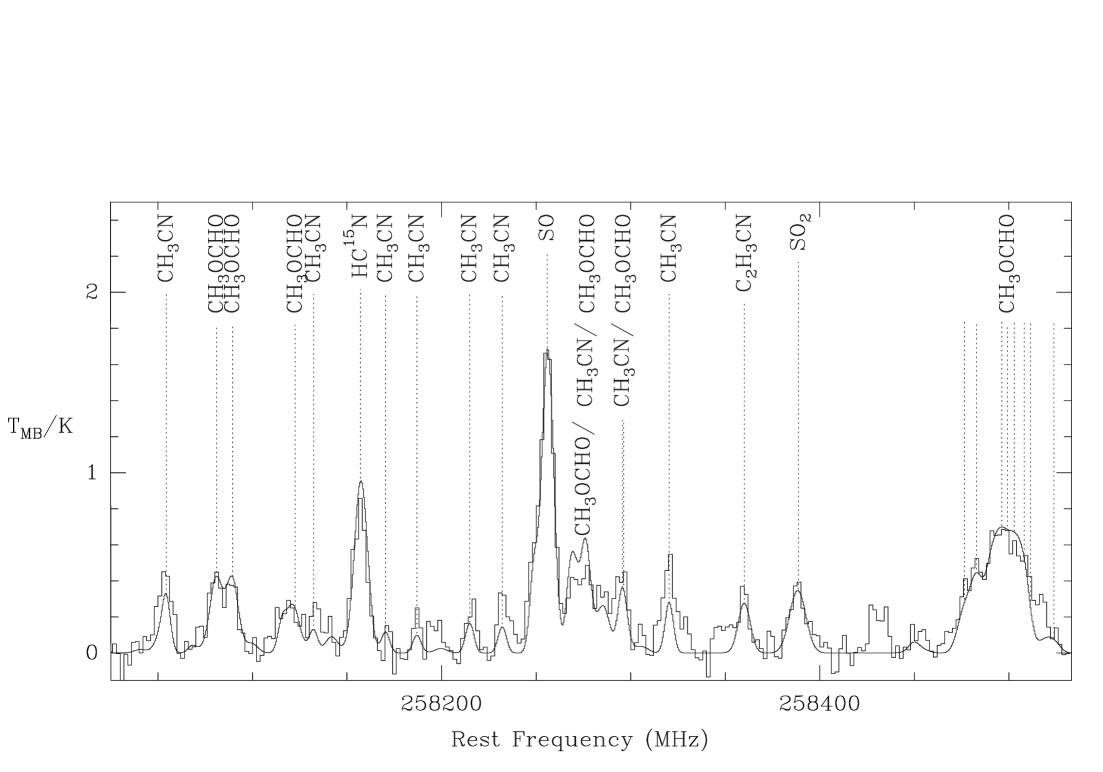
Figure 2: Sample spectrum of HCOOCH₃ in BAND1-HCN towards the source G10.47. We used the XCLASS software to solve the blending problem in this frequency band.

3.4 Vibrationally excited C₂H₃CN in G10.47

Several lines of vibrationally excited C₂H₃CN have been identified at 218 GHz (see Fig. 3) towards the source G10.47. The main line parameters are given in Table 5. These lines have been identified for the first time by Nummelin et al. (1998) in the Sagittarius B2 molecular cloud.

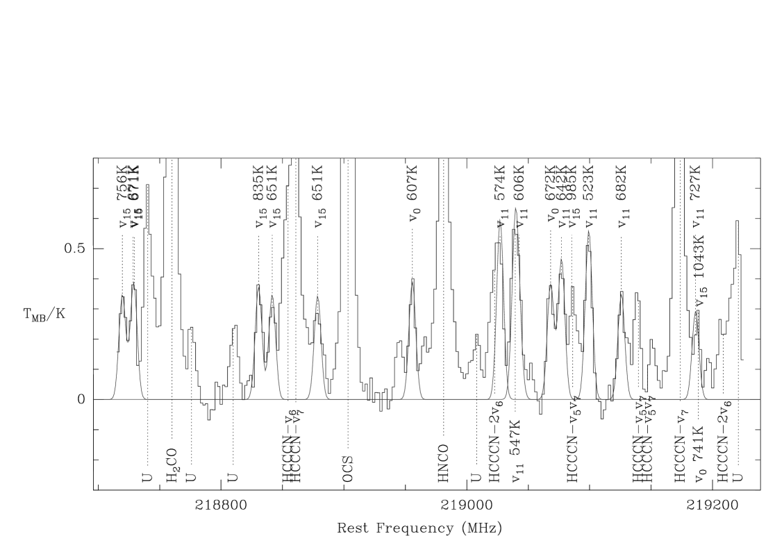
Figure 3: Vibrationally excited vinyl cyanide in G10.47 at 218 GHz. The lines are marked with their vibrational mode and upper energies are given.

The frequencies for the in-plane CCN bend $v_{11}$ at 342 K and the CCN out-of-plane bend $v_{15}$ at 486 K are taken from the JPL catalogue (Poynter & Pickett 1985, Pickett et al. 1996).

Table 5: Rest frequency ($\nu$), energy of the upper level ($E_{\rm u}$) and integrated intensity ($\int T_{\rm MB}{\rm d}v$) of 9 unblended vibrational lines of C₂H₃CN detected towards G10.47.

$\nu$	$E_{\rm u}$	$\int T_{\rm MB}{\rm d}v$
(MHz)	(K)	(K km s-1)
218719.6	756	3.23
218728.9	671	4.15
218830.5	835	3.57
218841.6	651	3.31
218878.6	651	3.28
219027.1	574	5.68
219077.1	642	4.71
219099.1	523	5.81
219125.8	682	3.46

Table 6: Rest frequency ($\nu$), energy of the upper level ($E_{\rm u}$) and integrated intensity ($\int T_{\rm MB}{\rm d}v$) of 12 unblended vibrational lines of C₂H₃CN detected towards G10.47 and G31.41.

Source	$\nu$	$E_{\rm u}$	$\int T_{\rm MB}{\rm d}v$
	(MHz)	(K)	(K km s-1)
G10.47	98464	410	2.0466
	98539	409	0.85978
	98619	361	5.3485
	98672	377	1.9452
	161338	422	3.4767
	224380	342	2.9466
	224396	616	2.1549
	224409	542	2.8934
	224480	522	2.7522
G31.41	98464	410	0.64
	98619	361	1.83
	98672	377	1.27
	98737	342	1.90
	161338	422	2.35
	224378	577	4.28
	224408	542	3.63
	224479	522	2.06

We also have found two ”weak” C₂H₃CN transitions (i.e. transitions with low $\mu^{2}$S, at $E_{\rm u}<$ 100 K, see Fig. 23). Both vibrational and “weak” lines are unlikely to be optically thick. Therefore, we combine them to derive both temperature and column density. We obtain a rotational temperature of 135 $\pm$ 13 K and a source averaged total column density of 1.3$\pm$0.6$\times 10^{18}$ cm^-2. The temperature is equal, within the error bar, to that given in Tab. 4 but the density is about a factor of 20 higher. Note that it is also a factor of 10 higher than C₂H₅CN column density (see Tab. 4). The presence of both ”weak” rotational and vibrational lines suggest that some ”strong” rotational transitions can suffer from high optical depth. Therefore, correcting the data following the method described in Sect. 3.2.4, we obtain a best fit for the following parameters: $N_{\rm s}\,=\,(2.3\,\pm\,0.4)\,\times\,10^{18}$ cm^-2, $T\,=\,133\,\pm\,3$ K, and $\theta\,\sim\,1.6$ ^′′.

3.5 Vibrationally excited C₂H₅CN in G10.47 and G31.41

Using the compilation of Pearson (2002), we have searched for vibrationally excited C₂H₅CN transitions. We have identified 9 lines in G10.47 and 8 in G31.41. In Fig. 4 and Fig. 5, we show the 3 bands in which vibrationally excited lines of C₂H₅CN have been identified. The main parameters of the identified lines are listed in Table 6. Vibrationally excited C₂H₅CN was firstly identified by Mehriger et al. (2004) in Sgr B2.

Figure 4: Bands in which vibrationally excited C₂H₅CN transitions have been identified (solid line) towards the source G10.47.

Figure 5: Bands in which vibrationally excited C₂H₅CN transitions have been identified (solid line) towards the source G31.41.

4 Discussion

4.1 Comparison between N-bearing and O-bearing molecules

A different spatial distribution between N-bearing and O-bearing molecules has been observed in some HMCs (see Blake et al. 1987, Wright et al. 1992, 1996, and Beuther et al. 2005 for Orion; Wyrowski et al. 1999 for W3(H₂O)). Caselli et al. (1993) interpreted the difference seen in Orion as being due to the fact that N-bearing and O-bearing species trace regions of the HMCs with different physical properties. Charnley et al. (1992) simply use different grain mantle compositions for the Orion-HC and Compact Ridge to reproduce the observed differentiation.

In order to see if such a differentiation is observable in the HMCs of our sample, we compare in each source the main physical properties (velocity, column density, temperature and abundance) obtained from N- and O-bearing species.

4.1.1 Line velocities and widths at half maximum

Peak velocities, $V_{\rm LSR}$, and line widths at half maximum, $\Delta V$, of the unblended lines detected in each source are listed in Cols. 3 and 4, respectively, of Table LABEL:tab:velocities. Both $V_{\rm LSR}$ and $\Delta V$ have been obtained from single Gaussian fits to the lines. In Cols. 2 and 3 of Table 8 we report the average values of $V_{\rm LSR}$ for the unblended lines of C₂H₅CN, $V_{\rm N}$, and CH₃OCH₃, $V_{\rm O}$, respectively, and their difference ($V_{\rm N}-V_{\rm O}$) is given in Col. 4. In Cols. 5, 6 and 7 of the same Table we also list the average value of the linewidths for C₂H₅CN, $\Delta V_{\rm N}$, and CH₃OCH₃, $\Delta V_{\rm O}$, and their ratio ($\Delta V_{\rm N}/\Delta V_{\rm O}$), respectively.

The velocity differences $V_{\rm N}-V_{\rm O}$ and line width ratios $\Delta V_{\rm N}/\Delta V_{\rm O}$ found in each source are then plotted in Fig. 6. $V_{\rm N}-V_{\rm O}$ shows that on average the C₂H₅CN lines have different velocities from the CH₃OCH₃ lines, in agreement with the idea that they are tracing different regions. The largest difference is for G10.62, for which however we stress that $V_{\rm N}$ has been derived from 3 lines only, and one of these (the line at 224045 MHz) has a very uncertain velocity. On the other hand, no systematic differences are present in the line widths, except for G19.61 for which the C₂H₅CN lines are more than $\sim 1.5$ times larger than the CH₃OCH₃ lines. We point out that the values plotted in Fig. 6 are average values between lines observed at different wavelenghts, and this can influence a lot the discussion of these quantities. In fact, the higher excitation lines, which trace the denser and hotter portion of the HMC, are also expected to have highest linewidths. Therefore, the number of unblended lines detected in each band, which are different for each source, may influence the average values both of velocities and linewidths. Also, each rotational transition of CH₃OCH₃ is split into four components coming from torsional motions of the molecule. The separation of these components in velocity is much smaller than the spectral resolution of our data, so that they are not resolved. Even though the software can derive the intrinsic $\Delta V$ and $V_{\rm LSR}$ from the theoretical separation of the different components, we believe that $\Delta V$ and $V_{\rm LSR}$ from these lines are less accurate than those derived from C₂H₅CN. For these reasons, we stress that the quantities plotted in Fig. 6 have to be interpreted carefully.

Figure 6: Top panel: difference between the average velocities of unblended transitions of C₂H₅CN ($V_{\rm N}$) and CH₃OCH₃ ($V_{\rm O}$). Bottom panel: ratio between the average line widths at half maximum of C₂H₅CN ($\Delta V_{\rm N}$) and CH₃OCH₃ ($\Delta V_{\rm O}$). Source code number is taken from Table 1.

4.1.2 Abundance correlations

The abundances relative to H₂ of C₂H₅CN, C₂H₃CN and CH₃OCH₃ are compared in Figure 7. For each pair of tracers, we have performed a least square fit to the data to check a possible correlation between the different abundances. The left panel of Figure 7 shows that the abundances of the two N-bearing molecules, C₂H₅CN and C₂H₃CN, are strongly correlated (correlation coefficient $r\sim 0.96$). This result agrees with the theoretical prediction that C₂H₃CN is producted through gas-phase reactions involving C₂H₅CN (Caselli et al. 1993). On the other hand, central and right panels of Figure 7 show that there is correlation also between the abundances of C₂H₅CN and C₂H₃CN, and that of CH₃OCH₃ (correlation coefficients $\sim 0.90$ and $\sim 0.86$, respectively). CH₃OCH₃ is thought to form both through reactions on grain surfaces (CH₃ + CH₃O $\rightarrow$ CH₃OCH₃, Allen & Robinson 1977), and in the gas phase through reactions between methanol and protonated methanol (Garrod & Herbst 2006), but both formation processes are not expected to involve species containing nitrogen. Furthermore, Bisschop et al. (2007) have indeed shown that in their HMCs the CH₃OCH₃ abundance does not correlate with that of other N-bearing species (see their Table 8). Neverthless, based on considerations about abundance ratios and temperatures, they suggest that the O- and N-bearing molecules observed in their work may have experienced a common formation scheme.

In Figure 8 we plot the molecular abundances against the total H₂ column densities. Even though the uncertainties on these quantities are large, Figure 8 shows that on average cores with higher H₂ column density have also larger column densities of C₂H₅CN, C₂H₃CN and CH₃OCH₃, without any substantial difference between O- and N-bearing species. We have also checked if a correlation is present between the observed abundances and the gas temperature: none of the sources show a correlation between these two parameters. In summary, we do not see any difference between CH₃OCH₃ and the two N-bearing species when comparing their abundances both to the gas temperature and density of the cores.

Figure 7: Comparison between the molecular abundances of C₂H₅CN and C₂H₃CN (left panel), C₂H₃CN and CH₃OCH₃ (central panel) and C₂H₅CN and CH₃OCH₃ (right panel). All abundances are relative to H₂. The solid lines correspond to the best-fits. The upper limit for the C₂H₃CN abundance in G10.62 is indicated by an arrow. Errorbars representing the typical uncertainties are shown in the lower right corners.

Figure 8: Comparison between the H₂ total column density and the molecular abundances of C₂H₅CN (left panel), C₂H₃CN (central panel) and CH₃OCH₃ (right panel). The upper limit for the C₂H₃CN abundance in G10.62 is indicated by an arrow. Errorbars representing the typical uncertainties are shown in the lower right corners.

4.1.3 Beam-averaged column densities and rotational temperatures

Figure 9 shows the ratios between the beam averaged column densities (top panel) and those between the rotational temperatures derived from C₂H₅CN and CH₃OCH₃ (see Tab. 4). The plot indicates that the column densities obtained from C₂H₅CN are on average marginally higher (a factor of $\sim 2.5$) than those derived from CH₃OCH₃ , suggesting that C₂H₅CN may indeed trace a region marginally denser than that traced by CH₃OCH₃. We note a significant (a factor of $\sim 11$) difference in G19.61, which is the source in which there is also the largest difference in linewidths between C₂H₅CN and CH₃OCH₃, suggesting that C₂H₅CN is actually associated with a denser and more turbulent sub-region of the HMC. On the other hand, no systematic difference is found in the rotational temperatures, with the significant exception of G10.62, for which we find a value more than 5 times higher from C₂H₅CN. However, for this source the temperature from CH₃OCH₃ is less accurate because it is derived from three transitions only.

Figs. 6,  7 and 9 do not allow to conclude that the O- and N-bearing species observed in this work trace different HMC regions. However, when discussing these results one has to bear in mind that the angular resolution of our data is much larger than the size of the HMC. High angular resolution observations have demonstrated that the environment of some of our HMCs, and in general of massive YSOs, has a complex structure, and may be fragmented in objects with different masses and in different evolutionary stages (see e.g. Garay et al. 1998 for G19.61; Avalos et al. 2006 and Mookerjea et al. 2007 for G34.26), whose angular separation is comparable to or even smaller than the angular resolution of the observations. The observed emission is hence affected both by the emission of other molecular condensations close to the main one and, less likely, by the emission of the cooler molecular gas of the envelope surrounding the HMC. Therefore, it is difficult to reveal a clear differentiation between O- and N-bearing species since the observed line parameters represent average values in the whole source.

Figure 9: Top panel: ratio between the beam averaged total column densities (N_b in Tab. 4) derived from C₂H₅CN and CH₃OCH₃. Bottom panel: ratio between the rotational temperatures derived from C₂H₅CN and CH₃OCH₃. The numbers on the x-axis indicate the identification number of each source as in Tab. 1. The dashed line represents equal column density or rotational temperature from C₂H₅CN and CH₃OCH₃.

Table 7: Line velocities ($V_{\rm LSR}$) and widths at half maximum ($\Delta V$) derived from single Gaussian fits to unblended lines for the sources G10.47, G10.62 and G19.61. The errors of the Gaussian fits to the lines are given between brackets.

Molecule	frequency	$V_{\rm LSR}$	$\Delta V$
	(MHz)	(km s-1)	(km s-1)
	G10.47
C2H5CN	98701.1090	67.249 (0.15)	8.411 (0.36)
	161581.2030	66.782 (0.48)	13.001 (1.37)
	161367.344	67.564 (0.37)	9.842 (0.86)
	224458.8590	66.546 (0.26)	10.180 (0.73)
	224419.8120	66.952 (0.35)	11.136 (1.12)
C2H3CN	147561.719	66.866 (0.49)	9.277 (1.20)
CH3OCH3	111783.241	66.745 (0.14)	9.939 (0.36)
	111782.596	66.754 (0.14)	9.555 (0.22)
	147456.863	66.940 (0.54)	13.100 (1.19)
	237620.371	65.184 (0.43)	11.751 (1.07)
	G10.62
C2H5CN	161581.203	-1.667 (0.82)	5.934 (1.51)
	224045.750	0.395 (0.35)	4.703 (0.78)
	224419.812	-1.409 (0.40)	6.208 (0.83)
C2H3CN	–	–	–
CH3OCH3	111783.241	-3.440 (0.28)	7.852 (0.58)
	111782.596	-3.429 (0.28)	7.357 (0.38)
	147210.732	-2.726 (0.27)	2.730 (0.57)
	237620.371	-2.615 (0.54)	5.690 (1.01)
	G19.61
C2H5CN	98701.109	39.665 (0.40)	10.119 (0.95)
	161581.203	40.198 (0.52)	12.758 (1.57)
	161367.344	43.908 (0.72)	9.451 (2.02)
	224045.750	39.835 (0.43)	6.861 (1.06)
	224419.812	40.334 (0.39)	7.634 (1.25)
C2H3CN	–	–	–
CH3OCH3	111783.241	41.429 (0.53)	5.955 (0.99)
	111782.596	41.427 (0.53)	5.264 (0.66)
	G29.96
C2H5CN	98701.109	97.792 (0.29)	4.721 (0.91)
	161581.203	97.413 (0.73)	7.728 (2.19)
	161367.344	98.110 (1.47)	11.032 (4.69)
	224045.750	98.124 (0.73)	6.617 (1.53)
	224419.812	97.169 (0.24)	2.854 (0.59)
	224458.859	96.595 (0.60)	5.633 (1.39)
C2H3CN	–	–	–
CH3OCH3	111783.241	97.929 (0.34)	5.675 (0.88)
	111782.596	97.976 (0.32)	4.919 (0.58)
	147210.732	105.190 (1.13)	10.947 (3.52)
	G31.41
C2H5CN	98701.109	97.711 (0.26)	8.289 (0.58)
	161581.203	97.179 (0.38)	8.365 (1.07)
	161367.344	97.006 (1.02)	8.245 (2.25)
	224458.859	96.673 (0.50)	9.998 (1.67)
	224419.812	97.140 (0.36)	9.065 (0.93)
C2H3CN	147561.719	97.316 (0.46)	9.643 (1.10)
CH3OCH3	111783.241	98.104 (0.06)	7.181 (0.15)
	111782.596	98.125 (0.06)	6.617 (0.10)
	147210.732	97.580 (0.18)	5.502 (0.49)
	173293.064	98.255 (0.36)	5.641 (0.83)
	237620.371	96.334 (0.20)	7.338 (0.46)
	G34.26
C2H5CN	98701.109	57.333 (0.26)	7.449 (0.66)
	161581.203	57.511 (0.34)	8.542 (0.93)
	161367.344	57.103 (0.53)	8.368 (1.46)
	224045.750	57.610 (0.39)	3.691 (0.92)
	224419.812	57.478 (0.34)	6.052 (0.81)
C2H3CN	–	–	–
CH3OCH3	111783.241	59.091 (0.11)	7.629 (0.25)
	111782.596	59.107 (0.10)	7.117 (0.16)
	147210.732	59.653 (0.35)	6.181 (0.84)
	173293.064	58.985 (0.27)	6.262 (0.72)
	237620.371	57.523 (0.17)	7.674 (0.38)

Table 8: Average line velocities and widths computed from the unblended lines of C₂H₅CN ($V_{\rm N}$ and $\Delta V_{\rm N}$, respectively) and CH₃OCH₃ ($V_{\rm O}$ and $\Delta V_{\rm O}$, respectively). Velocity differences ($V_{\rm N}-V_{\rm O}$) and linewidth ratios ($\Delta V_{\rm N}/\Delta V_{\rm O}$) are also given.

Source	$V_{\rm N}$	$V_{\rm O}$	$V_{\rm N}-V_{\rm O}$	$\Delta V_{\rm N}$	$\Delta V_{\rm O}$	$\Delta V_{\rm N}/\Delta V_{\rm O}$
	(km s-1)
G10.47	67.0	66.4	0.6	10.5	11.1	0.94
G10.62	–0.9	–3.1	–2.2	5.6	5.9	0.95
G19.61	40.8	41.4	–0.6	9.4	5.6	1.68
G29.96	97.5	97.9	–0.4	6.4	7.2	0.89
G31.41	97.1	97.7	–0.6	8.9	6.5	1.37
G34.26	57.4	58.9	–1.5	6.8	7.0	0.97

4.2 Hot core chemical ages

When comparing the observed abundance of different molecular species (see Sect. 3.2) from predictions of theoretical models, we can get some insights into the evolutionary stage of HMCs.

H-rich species are thought to form in icy mantles of dust grains and then released into the gas phase when the central massive (proto)star begins to heat up the surroundings. A following gas phase chemistry transforms many of the grain mantle products into other species. In particular, C₂H₅CN, formed onto dust grains and then evaporated, is expected to form C₂H₃CN through gas-phase reactions (Caselli et al. 1993). The occurrence of these reactions, as well as those which destroy C₂H₃CN, depends on the core physical parameters, which are thought to change with the core evolution. Therefore, the abundance ratio of C₂H₅CN and C₂H₃CN is correlated to the core evolutionary stage, and can be used as a ’chemical clock’ for the HMC.

In Col. 2 of Tab. 9 we list the observational values for the abundance ratio $R=X$(C₂H₃CN)/$X$(C₂H₅CN), derived from the molecule’s abundances given in Col. 6 of Table 4. We also plot these ratios in Fig. 10 together with the predictions of the chemical models of Caselli et al. (1993) for the Orion-HC and Compact Ridge. The physical and chemical properties of these two regions can be considered as ’extrema’ for our HMCs, so that we will use them to constrain the chemical ages of our sample. Chemical models predict a sharp decrease in the abundances of many complex molecules, among which are C₂H₃CN and C₂H₅CN, in HMCs after $\sim 10^{5}$ yrs (see Fig. 10). Therefore, the detection of several lines of both C₂H₃CN and C₂H₅CN suggest that all of our HMCs are likely younger than $\sim 10^{5}$ yrs. In fact, we find ages in the range from $\sim 3.7\times 10^{4}$ to $\sim 5.9\times 10^{4}$ yrs, with the HMC in G34.26 being the youngest and that in G29.96 the oldest. We point out that this procedure does not take into account the errors in the model predictions.

In Fig. 11 we also plot $R$ against the C₂H₅CN fractional abundance and we compare it with the theoretical curve predicted for the Orion HC. From Fig. 11 we deduce that the model underestimates the observed ratio by a factor greater than 10. This could be due to a missing reaction in the chemical network between C₂H₅CN and H₃O⁺. In fact, the hydronium ion is quite abundant in the HMC phase and could destroy some of the C₂H₅CN molecules, thus increasing the observed C₂H₃CN/C₂H₅CN abundance ratio (see e.g. Caselli et al. 1993). Another possibility is that additional C₂H₃CN forms in gas phase reactions as suggested by Charnley et al. (1992) and Rodgers & Charnley (2001).

Figure 10: Comparison between the observed abundance ratio of the daughter/parent pair C₂H₃CN /C₂H₅CN and the predictions of the chemical models of Caselli et al (1993). The observed abundance ratio of each source is plotted as a horizontal line (see the top right corner for the source identification). The curves correspond to the predictions of the models by Caselli et al. (1993) for the Orion-HC (corresponding to $T=200$ K and $n_{\rm H_{2}}=10^{7}$cm^-3) and Compact Ridge (corresponding to $T=100$ K and $n_{\rm H_{2}}=10^{6}$cm^-3).

Table 9: Hot cores chemical ages

Source	$R$	tmin	tmax
		($\times$104 yr)
G10.47	0.5$\pm$0.2	5.0	5.4
G19.61	0.4$\pm$0.2	4.7	5.0
G29.96	0.5$\pm$0.1	4.7	5.9
G31.41	0.4$\pm$0.1	4.3	4.7
G34.26	0.3$\pm$0.1	3.7	4.2
$R=X$(C2H3CN)/$X$(C2H5CN)

Figure 11: Observed abundance ratio $R=X$(C₂H₃CN)/$X$(C₂H₅CN) against C₂H₅CN fractional abundance. The solid line represents the prediction of the model by Caselli et al. (1993) for the Orion-HC ($T=200$ K, $n=10^{7}$ cm^-3). The numbers identify the sources as in Table 1.

4.3 Comments on individual sources

In this Section we describe the main properties of each source on the basis of the results obtained both in this work and from previous observations.

G10.47+0.03

In this region three UC Hiis are associated with a HMC (see e.g. Gibb et al. 2004). Observations of CH₃CN (13–12) and (19–18) (Hatchell et al. 1998) show that the temperature increases from $\sim$ 87 K at a distance of $\sim$ 2.3^′′ from the centre, to $\sim$ 134 K at 0.8^′′ from the centre, indicating a temperature gradient. This is confirmed by observations of the NH₃ (4,4) inversion transition (Cesaroni et al. 1998), that show temperature and velocity gradients, which can be interpreted in terms of a rotating structure with temperature increasing towards the centre. Our temperature measurements agree with the estimates obtained by Hatchell et al. (1998) at $\sim 1$^′′ from the core centre.

Fig. 6 indicates a small difference in the line velocities of O- and N-bearing molecules, suggesting that they are likely arising from marginally different regions. This result agrees with that of Olmi et al. (1996), who found a displacement between HCOOCH₃ and CH₃CN of $\sim$0.5^′′. The most surprising property of this source is the high C₂H₃CN column density. The presence of both vibrationally excited (see Sect. 3.4) and ”weak” b-type lines (see Sect. 3.2.4) suggest that C₂H₃CN is about 10 times more abundant than C₂H₅CN. If we use in the rotation diagram all our data (”strong”, ”weak” and vibrationally excited lines) and we correct for the optical depth (see Wyrowski et al. 1999 for the procedure) we obtain the following best fit parameters: N${}_{\rm s}\sim$ 1.7 $\times$ 10¹⁸ cm^-2, T${}_{\rm rot}\sim$ 140 K and $\theta\sim$ 1^′′. A previous study of vibrationally excited HC₃N also showed anomalous high abundance for this molecule, a column density of $\sim 4\times 10^{18}$ cm^-2, comparable with that from C₂H₃CN. This result is in agreement with the model predictions of Caselli et al. (1993), who showed that the abundances of HC₃N and C₂H₃CN, after evaporation from dust grains, vary in a very similar way both in the Orion-HC for $t>100$ yrs (see their Fig. 4) and in the Compact Ridge for $t\geq 10^{4}$ yrs (see their Fig. 5), while those of C₂H₅CN and HC₃N are very different between them. In fact, the destruction of C₂H₅CN by molecular ions (in particular H${}_{3}^{+}$) leads to the production of both C₂H₃CN and HC₃N via dissociative recombination of C₃H₄N⁺ (formed in the reaction with H${}_{3}^{+}$).

G10.62–0.38

This star forming region consists of a cluster of OB stars embedded in a dense, collapsing molecular cloud (Ho & Haschick 1986, Keto et al. 1987, 1988, Sollins et al. 2005). Keto et al. (1987) find an average temperature of 95 K for the absorption components at -3.0 and -0.5 km s^-1 and 140 K at 1.9 km s^-1, while the average temperature for the gas seen in emission, away from the UC Hii, is 54 K: they suggest a temperature decreasing from the HMC center with a power-law of the type R^-0.5. The temperature derived from C₂H₅CN (see Tab. 4) indicates that this molecule traces a region at about 0.1 pc from the centre of the core, which also coincides with the centre of the continuum emission of the UC Hii region. The C₂H₅CN and CH₃OCH₃ line velocities in Fig. 6 show that these molecules are spatially separated, with the latter more distant from the UC Hii. This is also suggested by the temperature derived from CH₃OCH₃, even though the statistics are very poor because only three lines at E${}_{u}<$ 100 K have been identified. We find only one blended transition of C₂H₃CN in all our spectra so we cannot estimate rotational temperature and column density for this molecule.

G19.61–0.23

This is a complex region with an irregular structure both of the ionized gas (Wood & Churchwell 1990), and of the molecular emission from the associated molecular clumps. Garay et al. (1998) found five distinct UC Hii regions excited by individual stars from VLA observations of the ionized and molecular gas (NH₃(2,2) inversion line): the cometary-like and most compact of them is associated with the densest ammonia clump, called Middle clump to distinguish it from the Northern and the Southwestern clumps. The Middle clump exhibits very broad line widths ($\sim$ 9.5 km s^-1) and is characterized by a $V_{\rm LSR}$ of $39.3\pm 0.1$ km s^-1 in the main NH₃(2,2) line: these values are similar to those we find for C₂H₅CN. The Southwestern clump shows lower $\Delta V$ and higher $V_{\rm LSR}$ equal to those for CH₃OCH₃. This seems to suggest that N- and O-bearing molecular emission originates from separate regions. This is confirmed by the column density ratio between C₂H₅CN and CH₃OCH₃, much higher than those of the other sources (see Fig. 9), suggesting that C₂H₅CN indeed traces a region denser than that traced by O-bearing species. In spite of this, high angular resolution observations of two rotational lines of C₂H₅CN and HCOOCH₃, performed with BIMA (Remijan et al. 2004), indicate that these molecules seem to trace the same region.

G29.96–0.02

G29.96 is an example of UC Hii cometary region. High angular resolution VLA observations in the ammonia (4,4) inversion transition (Cesaroni et al. 1998) show that the HMC has a nearly symmetric profile, and is not affected by the presence of the embedded UC Hii region. Our rotational temperatures agree with those obtained by Hatchell et al. (1998) from CH₃CN (13–12) and (19–18) and are higher than the estimate that they derive from CH₃OH ($T_{\rm rot}\sim 48$ K). This could indicate that O-bearing molecules map colder and extended gas. Nevertheless, Fig. 6 does not show any displacement between the location of O- and N-bearing molecules: both their $\Delta V$ and $V_{\rm LSR}$ are, in fact, equal within the error bars. This is supported by high angular resolution observations (Olmi et al. 2003) which have shown that some lines of HCOOCH₃ and the N-bearing molecule CH₃CN trace approximately the same region. Our $V_{\rm LSR}$ also agrees with those of C¹⁷O (2-1) and (3-2) measured by Hofner et al. (2000).

G31.41+0.31

The region is made of a core-halo UC Hii region, offset by $\sim 5$^′′ from a hot core in which Beltrán et al. (2005) have revealed a rotating toroidal structure. Also, as already mentioned in Sect. 3.1, they serendipitously detected the C₂H₅CN ($25_{2,24}-24_{2,23}$) and HCOOCH₃-A (25${}_{11,15}-26_{9,18}$) lines, and found from their high-angular resolution maps that, even though the two tracers peak at slightly different positions, their integrated emissions and that of the 1.4 mm continuum are fairly well overlapping. Interferometric observations of CH₃CN lines (Olmi et al. 1996; Beltrán et al. 2005) and of the NH₃(4,4) main and satellite inversion lines (Cesaroni et al. 1998) show that both the column density and the temperature increase towards the HMC center. This hot and dense gas has also been detected through HC₃N (17-16) in its v₇ and v₆ vibrationally excited states (Wyrowski et al. 1999). The ratio between the intensity of these two lines point to temperatures of $\sim$ 250 K.

Lower angular resolution maps of the CH₃CN (19-18) and (13-12) transitions (Hatchell et al. 1998) give a temperature in agreement with the estimate that we derive from our molecules (see Tab. 4). The $\Delta V$ of the CH₃CN lines are comparable to those measured by us from C₂H₅CN. CH₃OCH₃ and HCOOCH₃ have lower $\Delta V$, but the difference in $V_{\rm LSR}$ between the O- and N-bearing molecules is small.

G34.26+0.15

This is a complex massive star formation region located at a distance of 3.7 kpc (Kuchar & Bania 1994) extensively studied both in radio continuum (Wood & Churchwell 1989; Avalos et al. 2006) and in molecular lines (e.g. Garay & Rodríguez 1990; Hatchell et al. 1998; Sewilo et al. 2004). VLA observations of the NH₃ (2,2) and (3,3) inversion transitions (Garay & Rodríguez 1990) reveal the presence of three distinct regions of the molecular gas:

• a low density (n(H₂)$\simeq 10^{4}$ cm^-3), low-temperature (T${}_{\rm rot}\simeq 18$ K) gas in front of a bright cometary UC Hii region.

• a warm gas (T${}_{\rm rot}\simeq 70$ K) in a molecular disk-like structure $\simeq 7.3^{\prime\prime}\times 2.8^{\prime\prime}$ in size, mapped by the main hyperfine component of the (3,3) transition, seen in absorption.

• an ultracompact region $\simeq 1.6$^′′ in size, $\simeq 2$^′′ to the east of the bright cometary UC Hii region, traced by the satellite hyperfine lines of the (2,2) and (3,3) transitions. It is characterized by a rotational temperature of $185^{+75}_{-45}$ K and by a H₂ density of $\simeq 7\times 10^{7}$ cm^-3.

The H₂ density and temperatures estimated from the tracers studied in this paper agree with those given by Garay & Rodríguez (1990). Mookerjea et al. (2007) have observed with $\sim 1$^′′ resolution two transitions of C₂H₅CN, and one transition of CH₃OCH₃ and HCOOCH₃, but all of them fall out of the bands observed in this work. From these maps and those of other molecular species, Mookerjea et al. (2007) have concluded that O- and N-bearing species peak at different positions, separated by $\sim 0$$\aas@@fstack{\prime\prime}$8, with a spatial separation similar to that observed in Orion. Given the low angular resolution of our data and the complexity of the region, such a differentiation is not shown from our observations. Hatchell et al. (1998) found evidence for temperature and density gradient in this source: the high excitation CH₃CN (19-18) transitions trace a smaller, hotter and denser region than that traced by CH₃CN (13-12). Our C₂H₅CN and CH₃OCH₃ temperatures agree with those of the higher excitation lines, indicating that they trace the same hot gas.

5 Conclusions

We have surveyed rotational transitions of 4 complex O- and N-bearing molecules, C₂H₃CN, C₂H₅CN, CH₃OCH₃ and HCOOCH₃, with the IRAM-30m telescope towards a selected sample of 12 well-known HCs, all of them associated with UC Hii regions. For 6 sources of our sample, we have detected a sufficient number of transitions to derive the main physical properties of the cores. We focus our analysis on the 3 species C₂H₃CN, C₂H₅CN and CH₃OCH₃ only, because the HCOOCH₃ lines are usually blended. The main results of our study are summarised as follows:

• From the rotational lines of C₂H₃CN, C₂H₅CN and CH₃OCH₃, we have derived rotational temperatures from $\sim 100$ to $\sim 150$ K, and source averaged total column densities of order of $10^{15}-10^{17}$cm^-2. Temperatures and column densities derived from the three tracers are typically in good agreement among them in each source, indicating that they are tracing approximately the same dense and hot gas of the cores.

• The abundances relative to H₂ are of the order of $\sim 10^{-9}-10^{-10}$ for all species, and are comparable to the values found in the Orion-hot core and in Sgr B2. The C₂H₅CN abundances are also comparable to those derived in other HMCs by Bisschop et al. (2007), while for CH₃OCH₃ we find values a factor of $\sim 2.5$ lower. There is a strong correlation between the abundances of C₂H₅CN and C₂H₃CN, as expected from theory that predicts that the latter is formed through gas phase reactions involving C₂H₅CN. Interestingly, a correlation is present also between the two N-bearing species and CH₃OCH₃, in disagreement with the results found by Bisschop et al. (2007) in similar sources.

• Single Gaussian fits to unblended lines reveal a small difference between the average peak velocity of C₂H₅CN and CH₃OCH₃ lines, suggesting a possible spatial separation of the two tracers, as seen in Orion and W3(H₂O). On the other hand, no systematic differences are found in the linewidths. We find a clear difference only in G19.61. We believe that this partly is due to the poor angular resolution of our observations, which allows us to derive only average values over the sources, which show a complex morphology.

• We have compared the abundance ratio of the daughter/parent pair C₂H₅CN/C₂H₃CN with the predictions of chemical models to constrain the HCs’ chemical ages. We find ages between 3.7-5.9$\times 10^{4}$ yrs. We also compared this ratio against C₂H₅CN  fractional abundance, finding that chemical models understimate even by a factor greater than 10 our observational results.

The chemical and physical differentiation between O- and N-bearing molecules seen in the Orion HC and W3(H₂O) is not revealed by our observations of other HMCs. We stress however that our data have beam size much larger than the diameters of the HMCs, providing only average values of the physical parameters of interest in the whole molecular clump hosting the cores, and may be affected by other objects embedded inside the clumps themselves. Follow-up observations with millimeter and sub-millimeter interferometers (in particular ALMA, available in the near future) will be fundamental to provide maps with resolution comparable or even smaller than the core sizes, thus allowing us to derive with better spatial accuracy the physical parameters of the HMCs.

Appendix A: Observed spectra

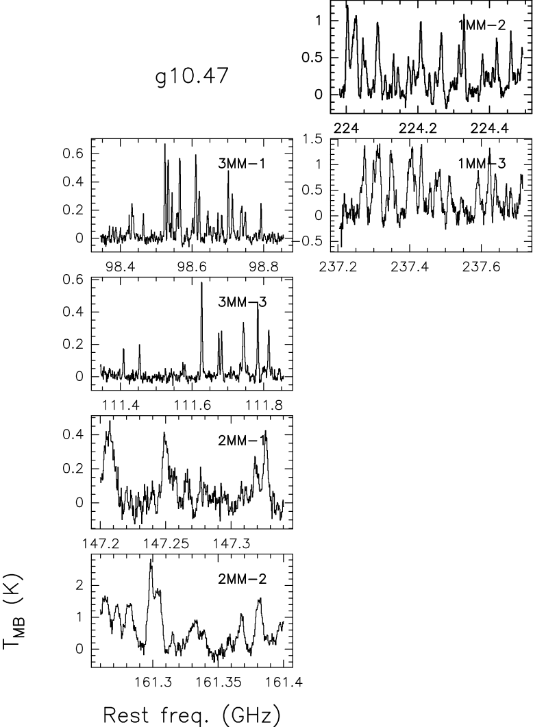
Figure 12: Spectra obtained towards G10.47 with the IRAM-30m Telescope during the 1997 observing run.

Figure 13: Spectra obtained towards G10.47 with the IRAM-30m Telescope during the 1996 observing run.

Figure 14: Same as Fig. 12 for G10.62.

Figure 15: Same as Fig. 13 for G10.62.

Figure 16: Same as Fig. 12 for G19.61.

Figure 17: Same as Fig. 12 for G29.96.

Figure 18: Same as Fig. 13 for G29.96.

Figure 19: Same as Fig. 12 for G31.41.

Figure 20: Same as Fig. 13 for G31.41.

Figure 21: Same as Fig. 12 for G34.26.

Figure 22: Same as Fig. 13 for G34.26.

Appendix B: Tables

Tables LABEL:tab:g1042007–20 list the molecular transitions used to derive the rotational temperatures and total column densities of the sources in Table 3. For each line we give: rest frequency, $\nu$, in MHz (Col. 1, indicated with ”b” if it is a b-type transition); the molecular species (Col. 2); the energy of the lower level, $E_{\rm l}$, in cm^-1 (Col. 3); the line integrated emission, $\int T_{MB}\>dv$, in K km s^-1; (Col. 4); the quantity $\mu^{2}S$, where $\mu$ (in Debye) is the molecule’s dipole moment and $S$ is the line strength (Col. 5). The CH₃OCH₃ lines are separated in four components not resolved in our spectra (see also Sect. 4.1). For this reason, for the CH₃OCH₃ transitions we give in Col. 4 the total integrated emission of the four components divided by the sum of the statistical weights of each component (for the statistical weights see Groner et al. 1998).

Table 10: Transitions observed towards G10.47 during the 1997 observing run.

$\nu$	Molecule	$E_{\rm l}$	$\int{T_{MB}}\>dv$	$\mu^{2}S$
(MHz)		(cm-1)	(K km s-1)	$(D^{2})$
b98399.6170	C2H3CN	66.0140	0.498	4.682
98523.883	C2H5CN	44.251	3.33	113.939
98524.664	C2H5CN	54.287	3.05	96.525
98532.070	C2H5CN	65.860	3.19	76.412
98533.9845	C2H5CN	35.754	4.16	128.685
98544.148	C2H5CN	78.967	2.78	53.615
98559.867	C2H5CN	93.604	1.64	28.149
98564.836	C2H5CN	28.801	4.11	140.761
98566.797	C2H5CN	28.801	3.15	140.761
98701.109	C2H5CN	23.398	4.38	150.140
b111574.6250	C2H5CN	73.7330	0.74	10.807
b111783.241	CH3OCH3	17.550	0.1439	27.2197
b111802.549	CH3OCH3	42.142	0.0287	4.43093
b111813.417	CH3OCH3	118.013	0.1204	96.5637
b147205.839	CH3OCH3	22.082	0.2271	19.52177
b147456.863	CH3OCH3	257.141	0.1097	145.57157
147561.719	C2H3CN	38.4910	4.70	232.515
161261.141	C2H5CN	95.144	13.0	213.000
161265.734	C2H5CN	108.253	12.5	199.066
b161281.953	CH3OCH3	75.305	0.3944	49.41313
161289.996	CH3OCH3	333.668	0.1341	162.13361
161303.484	C2H5CN	139.060	9.28	166.301
161304.922	C2H5CN	73.536	11.3	235.930
161367.344	C2H5CN	175.957	9.38	126.974
161380.828	C2H5CN	101.33	15.13	246.2506
161397.047	C2H3CN	97.1140	6.92	217.164
161441.2660	C2H3CN	139.0100	5.87	386.26
161445.3910	C2H3CN	67.1130	7.04	234.339
161450.3590	C2H3CN	67.1130	7.04	234.339
161475.172	C2H5CN	52.712	19.70	258.004
161502.266	C2H3CN	56.6050	9.00	240.337
161516.7190	C2H5CN	58.1110	9.38	252.312
161527.500	C2H3CN	192.6770	5.77	162.238
161581.203	C2H5CN	58.115	14.3	252.312
161582.047	C2H3CN	223.8800	3.37	144.202
161643.250	C2H3CN	257.9690	4.50	124.459
224002.109	C2H5CN	166.828	4.40	309.672
224003.438	C2H5CN	152.185	6.00	320.879
224045.750	C2H5CN	200.696	5.73	283.720
224084.281	C2H5CN	219.912	5.20	268.960
224088.2035	C2H5CN	127.510	6.00	339.753
224131.516	C2H5CN	240.640	3.63	253.034
224186.344	C2H5CN	262.876	3.27	235.930
224206.609	C2H5CN	117.492	4.09	347.406
224208.078	C2H5CN	117.492	4.09	347.406
b224231.6880	C2H5CN	94.4160	2.05	33.527
224248.016	C2H5CN	286.614	2.21	217.645
224389.719	C2H5CN	338.567	2.25	177.537
224419.812	C2H5CN	109.033	6.34	353.894
224458.859	C2H5CN	109.036	8.10	353.894
b237360.8910	C2H5CN	114.9850	2.33	24.209
237396.9765	C2H3CN	168.5260	5.15	336.209
237405.1880	C2H5CN	101.8870	13.71	380.894
237456.2500	C2H3CN	216.3420	5.07	635.06
237482.766	C2H3CN	132.5690	4.06	350.218
237485.016	C2H3CN	132.5700	3.61	350.218
237548.541	CH3OCH3	447.259	0.200	34.69413
237585.484	C2H3CN	275.8720	3.58	294.183
237591.391	C2H3CN	108.5880	6.11	359.528
b237620.371	CH3OCH3	32.291	0.551	23.17836
237638.0160	C2H3CN	119.0860	6.74	355.471
237668.766	C2H3CN	309.9800	4.29	280.758

Table 11: Transitions observed towards G10.47 during the 1996 observing run.

$\nu$	Molecule	$E_{\rm l}$	$\int{T_{MB}}\>dv$	$\mu^{2}S$
(MHz)		(cm-1)	(K km s-1)	$(D^{2})$
b140163.0	CH3OCH3	308.85	0.1086	23.138
b140226.172	CH3OCH3	159.81	0.0911	9.896
a140429.484	C2H3CN	54.24	8.45	202.872
b154027.062	C2H3CN	10.02	4.68	2.344
a154724.531	C2H3CN	65.42	9.77	215.731
b154311.469	CH3OCH3	185.5	0.0667	12.855
b154456.5	CH3OCH3	62.92	0.4117	21.739
215040.8	C2H5CN	229.5	24.1	1199.4
215088.203	C2H5CN	288.76	15.5	533.6
215109.047	C2H5CN	183.46	19.7	651.1
215119.203	C2H5CN	135.84	16.5	369.7
215126.703	C2H5CN	316.4	10.0	502.8
215400.797	C2H5CN	156.87	17.6	340.3
215427.984	C2H5CN	156.88	19.0	340.332
227897.625	C2H3CN	242.47	13.12	594.744
227906.719	C2H3CN	214.46	10.29	609.457
227918.656	C2H3CN	274.75	9.18	577.798
227960.234	C2H3CN	311.27	7.23	558.56
227967.594	C2H3CN	190.74	19.11	621.8
228017.375	C2H3CN	352.	10.23	537.313
228087.297	C2H3CN	396.91	6.95	513.431
228090.531	C2H3CN	156.23	8.88	319.903
228104.609	C2H3CN	171.34	11.91	315.959
228160.297	C2H3CN	171.35	16.7	631.917

Table 12: Transitions observed towards G10.62–0.38 during the 1997 observing run.

$\nu$	Molecule	$E_{\rm l}$	$\int{T_{MB}}\>dv$	$\mu^{2}S$
(MHz)		(cm-1)	(K km s-1)	$(D^{2})$
b111783.241	CH3OCH3	17.550	0.0403	27.2197
111802.17	CH3OCH3	42.141	0.016	2.53886
111802.93	CH3OCH3	42.142	0.013	2.53886
111813.417	CH3OCH3	118.013	0.016	96.5637
b147205.839	CH3OCH3	22.082	0.0478	19.52177
147456.863	CH3OCH3	257.141	0.0196	145.57157
161261.141	C2H5CN	95.144	1.82	213.000
161265.734	C2H5CN	108.253	0.32	199.066
161281.953	CH3OCH3	75.305	0.0572	49.41313
161289.996	CH3OCH3	333.668	0.0572	162.13361
161475.172	C2H5CN	52.712	0.86	258.004
161581.203	C2H5CN	58.115	1.07	252.312
224002.109	C2H5CN	166.828	0.78	309.672
224003.438	C2H5CN	152.185	0.97	320.879
224045.750	C2H5CN	200.696	0.65	283.720
224084.281	C2H5CN	219.912	0.39	268.960
224088.2035	C2H5CN	127.510	1.16	339.753
224206.609	C2H5CN	117.492	1.05	347.406
224208.078	C2H5CN	117.492	0.67	347.406
224419.812	C2H5CN	109.033	1.20	353.894
224458.859	C2H5CN	109.036	1.05	353.894
237261.970	CH3OCH3	214.188	0.117	66.88355
237548.541	CH3OCH3	447.259	0.117	34.69413
b237620.371	CH3OCH3	32.291	0.0875	23.17836

Table 13: Transitions observed towards G10.62–0.38 during the 1996 July observing run.

$\nu$	Molecule	$E_{\rm l}$	$\int{T_{MB}}\>dv$	$\mu^{2}S$
(MHz)		(cm-1)	(K km s-1)	$(D^{2})$
215040.8	C2H5CN	229.5	2.49	1199.4
215109.047	C2H5CN	183.46	3.25	651.1
215427.984	C2H5CN	156.88	1.67	340.332

Table 14: Transitions observed towards G19.61–0.23 during the 1997 observing run.

$\nu$	Molecule	$E_{\rm l}$	$\int{T_{MB}\>dv}$	$\mu^{2}S$
(MHz)		(cm-1)	(K km s-1)	$(D^{2})$
98523.883	C2H5CN	44.251	1.24	113.939
98524.664	C2H5CN	54.287	0.87	96.525
98532.070	C2H5CN	65.860	0.75	76.412
98533.9845	C2H5CN	35.754	1.49	128.685
98544.148	C2H5CN	78.967	0.69	53.615
98564.836	C2H5CN	28.801	1.21	140.761
98566.797	C2H5CN	28.801	0.72	140.761
98701.109	C2H5CN	23.398	1.24	150.140
b104177.000	CH3OCH3	102.625	0.185	79.56847
104212.656	C2H3CN	23.4110	0.80	155.205
104419.312	C2H3CN	71.4640	0.80	112.653
104432.797	C2H3CN	30.9450	0.72	148.58
104437.516	C2H3CN	90.9290	0.94	95.507
104453.930	C2H3CN	30.9460	0.72	148.58
104490.168	CH3OCH3	585.600	0.026	4.48006
b111783.241	CH3OCH3	17.550	0.017	27.2197
b111813.417	CH3OCH3	118.013	0.024	96.5637
147205.839	CH3OCH3	22.082	0.0376	19.52177
147456.863	CH3OCH3	257.141	0.0376	145.57157
147561.719	C2H3CN	38.4910	2.46	232.515
161261.141	C2H5CN	95.144	5.56	213.
161265.734	C2H5CN	108.253	4.72	199.066
b161281.953	CH3OCH3	75.305	0.0483	49.41313
161289.996	CH3OCH3	333.668	0.0512	162.13361
161303.484	C2H5CN	139.060	3.33	166.301
161304.922	C2H5CN	73.536	3.89	235.93
161367.344	C2H5CN	175.957	2.78	126.974
161379.844	C2H5CN	65.047	2.79	244.939
161397.0470	C2H3CN	97.1140	2.84	434.328
161381.875	C2H5CN	65.047	2.79	244.939
161441.266	C2H3CN	139.0100	2.21	193.130
161445.391	C2H3CN	67.1130	2.94	234.339
161475.172	C2H5CN	52.712	5.04	258.004
161480.219	C2H3CN	164.3800	3.68	178.538
161527.500	C2H3CN	192.6770	1.10	162.238
161581.203	C2H5CN	58.115	4.78	252.312
209422.190	CH3OCH3	136.101	0.1111	71.12975
209515.532	CH3OCH3	41.221	0.1111	54.9886
209735.828	C2H3CN	86.7860	1.14	315.05
209812.329	CH3OCH3	168.885	0.0864	64.85627
224002.109	C2H5CN	166.828	4.21	309.672
224003.438	C2H5CN	152.185	7.58	320.879
224045.750	C2H5CN	200.696	4.21	283.72
224084.281	C2H5CN	219.912	2.95	268.96
224088.203	C2H5CN	127.510	8.01	339.753
224186.344	C2H5CN	262.876	2.63	235.93
224206.609	C2H5CN	117.492	4.01	347.406
224208.078	C2H5CN	117.492	4.01	347.406
224419.812	C2H5CN	109.033	6.01	353.894
224458.859	C2H5CN	109.036	6.01	353.894
237261.970	CH3OCH3	214.188	0.1533	66.88355
237396.976	C2H3CN	168.5260	3.14	336.209
237411.906	C2H3CN	149.0560	3.14	343.797
237415.359	C2H3CN	190.9600	2.62	327.453
237456.250	C2H3CN	216.3420	2.32	317.531
237483.891	C2H3CN	132.5690	2.98	700.436
237514.016	C2H3CN	244.6530	1.85	306.440
237548.541	CH3OCH3	447.259	0.1533	34.69413
237585.4840	C2H3CN	275.8720	2.04	588.366
237591.3910	C2H3CN	108.5880	2.38	359.528
237620.371	CH3OCH3	32.291	0.1533	23.17836
237638.016	C2H3CN	119.0860	3.49	355.471

Table 15: Transitions observed towards G29.96–0.02 during the 1997 observing run.

$\nu$	Molecule	$E_{\rm l}$	$\int{T_{MB}\>dv}$	$\mu^{2}S$
(MHz)		(cm-1)	(K km s-1)	$(D^{2})$
98523.883	C2H5CN	44.251	0.41	113.939
98524.664	C2H5CN	54.287	0.52	96.525
98532.070	C2H5CN	65.860	0.34	76.412
98533.9845	C2H5CN	35.754	0.55	128.685
98564.836	C2H5CN	28.801	0.19	140.761
98566.797	C2H5CN	28.801	0.40	140.761
98701.109	C2H5CN	23.398	0.69	150.140
104177.000	CH3OCH3	102.625	0.021	79.56847
104490.168	CH3OCH3	585.600	0.027	4.48006
104437.5160	C2H3CN	90.9290	0.353	191.014
111802.17	CH3OCH3	42.141	0.024	2.53886
111802.93	CH3OCH3	42.142	0.0183	2.53886
b111813.417	CH3OCH3	118.013	0.0368	96.5637
b147205.839	CH3OCH3	22.082	0.0458	19.52177
147456.863	CH3OCH3	257.141	0.040	145.57157
161261.141	C2H5CN	95.144	2.14	213.0
161265.734	C2H5CN	108.253	1.16	199.066
161289.996	CH3OCH3	333.668	0.0467	162.13361
161303.484	C2H5CN	139.060	2.14	166.301
161304.922	C2H5CN	73.536	1.43	235.930
161367.344	C2H5CN	175.957	1.79	126.974
161379.844	C2H5CN	65.047	1.34	244.939
161381.875	C2H5CN	65.047	1.34	244.939
161397.047	C2H3CN	97.1140	0.89	217.164
161475.172	C2H5CN	52.712	1.63	258.004
161480.219	C2H3CN	164.3800	0.71	178.538
161581.203	C2H5CN	58.115	1.59	252.312
173083.162	CH3OCH3	110.480	0.1542	34.27361
173094.261	CH3OCH3	149.025	0.1542	85.5836
173293.064	CH3OCH3	34.233	0.1542	46.73276
209735.8280	C2H3CN	86.7860	0.73	315.05
209422.190	CH3OCH3	136.101	0.094	71.12975
209515.532	CH3OCH3	41.221	0.094	54.9886
209812.329	CH3OCH3	168.885	0.0733	64.85627
224002.109	C2H5CN	166.828	1.86	309.672
224003.438	C2H5CN	152.185	1.72	320.879
224017.5310	C2H5CN	183.0000	1.21	594.572
224028.1410	C2H5CN	139.0770	1.08	661.812
224045.750	C2H5CN	200.696	2.19	283.720
224084.281	C2H5CN	219.912	2.09	268.960
224088.2035	C2H5CN	127.510	2.00	339.753
224206.609	C2H5CN	117.492	2.36	347.406
224208.078	C2H5CN	117.492	1.68	347.406
224419.812	C2H5CN	109.033	2.86	353.894
224458.859	C2H5CN	109.036	2.36	353.894
237261.970	CH3OCH3	214.188	0.146	66.88355
237396.976	C2H3CN	168.526	1.22	336.209
237548.541	CH3OCH3	447.259	0.146	34.69413
237620.371	CH3OCH3	32.291	0.146	23.17836

Table 16: Transitions observed towards G29.96-0.02 during the 1996 observing run.

$\nu$	Molecule	$E_{\rm l}$	$\int{T_{MB}\>dv}$	$\mu^{2}S$
(MHz)		(cm-1)	(K km s-1)	$(D^{2})$
b154311.469	CH3OCH3	185.5	0.0114	12.859
b154456.5	CH3OCH3	62.92	0.063	21.739
215040.8	C2H5CN	229.5	5.22	1199.4
215088.203	C2H5CN	288.76	2.31	533.6
215109.047	C2H5CN	183.46	4.82	651.1
215119.203	C2H5CN	135.84	4.22	369.666
215126.703	C2H5CN	316.4	1.66	502.8
215173.234	C2H5CN	346.23	1.5	469.4
215400.797	C2H5CN	156.87	3.44	340.336
215427.984	C2H5CN	156.88	3.88	340.332

Table 17: Transitions observed towards G31.41+0.31 during the 1997 August observing run.

$\nu$	Molecule	$E_{\rm l}$	$\int{T_{MB}\>dv}$	$\mu^{2}S$
(MHz)		(cm-1)	(K km s-1)	$(D^{2})$
98523.883	C2H5CN	44.251	1.60	113.939
98524.664	C2H5CN	54.287	2.00	96.525
98532.070	C2H5CN	65.860	1.80	76.412
98533.9845	C2H5CN	35.754	2.79	128.685
98544.148	C2H5CN	78.967	2.22	53.615
98559.867	C2H5CN	93.604	0.59	28.149
98564.836	C2H5CN	28.801	1.87	140.761
98566.797	C2H5CN	28.801	2.42	140.761
98701.109	C2H5CN	23.398	2.60	150.140
b104177.000	CH3OCH3	102.625	0.0843	79.56847
104212.656	C2H3CN	23.411	1.18	155.205
104419.312	C2H3CN	71.464	1.48	112.653
104432.7970	C2H3CN	30.9450	1.13	148.58
104453.930	C2H3CN	30.9460	1.62	148.580
104490.168	CH3OCH3	585.600	0.0424	4.48006
b 111574.6250	C2H5CN	73.7330	0.38	10.807
b111742.636	CH3OCH3	130.299	0.1514	103.90668
b111783.241	CH3OCH3	17.550	0.1647	27.2197
b111801.945	CH3OCH3	42.142	0.029	4.43093
b111813.417	CH3OCH3	118.013	0.1694	96.5637
b147205.839	CH3OCH3	22.082	0.3239	19.52177
b147456.863	CH3OCH3	257.141	0.0816	145.57157
147561.719	C2H3CN	38.4910	2.66	232.515
161261.141	C2H5CN	95.144	7.89	213.
161265.734	C2H5CN	108.253	6.91	199.066
b161281.953	CH3OCH3	75.305	0.1839	49.41313
161289.996	CH3OCH3	333.668	0.0667	162.13361
161303.484	C2H5CN	139.060	5.67	66.301
161304.922	C2H5CN	73.536	3.70	235.93
161367.344	C2H5CN	175.957	2.47	126.974
161379.844	C2H5CN	65.047	3.86	244.939
161381.875	C2H5CN	65.047	4.12	244.939
161397.047	C2H3CN	97.114	3.62	217.164
161447.8750	C2H3CN	67.1130	5.4	468.678
161475.172	C2H5CN	52.712	8.24	258.004
161502.266	C2H3CN	56.605	2.16	240.337
161581.203	C2H5CN	58.115	5.92	252.312
172998.766	C2H5CN	55.578	9.50	293.998
173092.859	C2H3CN	54.7720	11.2	259.424
173083.162	CH3OCH3	110.480	0.3097	34.27361
173094.261	CH3OCH3	149.025	0.1542	85.5836
b173293.064	CH3OCH3	34.233	0.4182	46.73276
b209515.532	CH3OCH3	41.221	0.479	54.9886
209812.329	CH3OCH3	168.885	0.1334	64.85627
224002.109	C2H5CN	166.828	5.36	309.672
224003.438	C2H5CN	152.185	6.13	320.879
224045.75	C2H5CN	200.696	6.72	283.720
224084.281	C2H5CN	219.912	4.60	268.960
224088.2035	C2H5CN	127.510	6.89	339.753
224131.516	C2H5CN	240.640	3.82	253.034
224186.344	C2H5CN	262.876	3.73	235.930
224206.609	C2H5CN	117.492	5.22	347.406
224208.078	C2H5CN	117.492	5.22	347.406
224248.016	C2H5CN	286.614	1.91	217.645
224419.812	C2H5CN	109.033	7.66	353.894
224458.859	C2H5CN	109.036	7.63	353.894
237396.9765	C2H3CN	168.526	2.50	336.209
237405.1880	C2H5CN	101.8870	8.49	380.894
b237476.0470	C2H5CN	91.4820	3.77	19.864
237456.250	C2H3CN	216.3420	2.10	317.531
237485.016	C2H3CN	132.5700	3.12	350.218
237548.541	CH3OCH3	447.259	0.1445	34.69413
237591.3910	C2H3CN	108.5880	2.17	359.528
b237620.371	CH3OCH3	32.291	0.452	23.17836
237638.0160	C2H3CN	119.0860	2.17	355.471
237668.7660	C2H3CN	309.9800	2.03	561.516

Table 18: Transitions observed towards G31.41+0.31 during the 1996 July observing run.

$\nu$	Molecule	$E_{\rm l}$	$\int{T_{MB}}\>dv$	$\mu^{2}S$
(MHz)		(cm-1)	(K km s-1)	$(D^{2})$
b140226.172	CH3OCH3	159.81	0.0686	9.896
a140429.484	C2H5CN	54.24	2.2	202.872
b154027.062	C2H5CN	10.02	2.64	2.344
b154311.469	CH3OCH3	185.5	0.035	12.855
b154456.5	CH3OCH3	62.92	0.2081	21.739
154724.531	C2H5CN	65.42	5.75	215.731
215040.8	C2H5CN	229.5	15.9	1199.4
215088.203	C2H5CN	288.76	8.46	533.6
215109.047	C2H5CN	183.46	12.49	651.1
215119.203	C2H5CN	135.84	12.63	369.666
215126.703	C2H5CN	316.4	6.56	502.8
215173.234	C2H5CN	346.23	5.91	469.4
215400.797	C2H5CN	156.87	11.84	340.336
215427.984	C2H5CN	156.88	12.85	340.332
227897.625	C2H5CN	242.47	6.59	594.744
227906.719	C2H5CN	214.46	6.89	609.457
227918.656	C2H5CN	274.75	3.33	577.798
227960.234	C2H5CN	311.27	3.03	558.56
227967.594	C2H5CN	190.74	6.87	621.8
228017.375	C2H5CN	352.	3.44	537.313
228087.297	C2H5CN	396.91	0.91	513.431
228090.531	C2H5CN	156.23	5.45	319.903
228104.609	C2H5CN	171.34	5.45	315.959
228160.297	C2H5CN	171.35	7.02	631.917

Table 19: Transitions observed towards G34.26+0.15 during the 1997 observing run.

$\nu$	Molecule	$E_{\rm l}$	$\int{T_{MB}\>dv}$	$\mu^{2}S$
(MHz)		(cm-1)	(K km s-1)	$(D^{2})$
98523.883	C2H5CN	44.251	1.23	113.939
98524.664	C2H5CN	54.287	0.96	96.525
98532.070	C2H5CN	65.860	1.16	76.412
98533.9845	C2H5CN	35.754	1.64	128.685
98544.148	C2H5CN	78.967	0.68	53.615
98559.867	C2H5CN	93.604	0.24	28.149
98564.836	C2H5CN	28.801	1.10	140.761
98566.797	C2H5CN	28.801	1.35	140.761
98701.109	C2H5CN	23.398	1.37	150.140
b104177.000	CH3OCH3	102.625	0.1033	79.56847
104419.312	C2H3CN	71.4640	0.57	112.653
104432.797	C2H3CN	30.9450	0.57	148.58
104437.516	C2H3CN	90.9290	0.71	95.507
104453.930	C2H3CN	30.9460	0.89	148.58
104461.5160	C2H3CN	113.3510	0.425	151.236
b111783.241	CH3OCH3	17.550	0.1639	27.2197
111802.93	CH3OCH3	42.142	0.0192	2.53886
b111813.417	CH3OCH3	118.013	0.1493	96.5637
b147205.839	CH3OCH3	22.082	0.2814	19.52177
b147456.863	CH3OCH3	257.141	0.0763	145.57157
161261.141	C2H5CN	95.144	9.19	213.
161265.734	C2H5CN	108.253	6.32	199.066
b161285.603	CH3OCH3	75.305	0.279	12.35331
161289.996	CH3OCH3	333.668	0.0566	162.13361
161303.484	C2H5CN	139.060	6.89	166.301
161304.922	C2H5CN	73.536	6.89	235.930
161367.344	C2H5CN	175.957	2.87	126.974
161379.844	C2H5CN	65.047	6.24	244.939
161381.875	C2H5CN	65.047	4.05	244.939
161397.047	C2H3CN	97.1140	2.31	217.164
161445.391	C2H3CN	67.1130	2.21	234.339
161450.359	C2H3CN	67.1130	2.21	234.339
161475.172	C2H5CN	52.712	7.47	258.004
161581.203	C2H5CN	58.115	5.75	252.312
172998.766	C2H5CN	55.578	5.92	293.998
173092.859	C2H3CN	54.7720	4.69	259.424
b173293.064	CH3OCH3	34.233	0.3016	46.73276
b209515.532	CH3OCH3	41.221	0.7994	54.9886
b209812.329	CH3OCH3	168.885	0.1865	64.85627
224002.109	C2H5CN	166.828	9.23	309.672
224003.438	C2H5CN	152.185	3.69	320.879
224045.75	C2H5CN	200.696	3.26	283.720
224084.281	C2H5CN	219.912	3.88	268.960
224088.2035	C2H5CN	127.510	6.79	339.753
224186.344	C2H5CN	262.876	2.43	235.930
224206.609	C2H5CN	117.492	4.95	347.406
224208.078	C2H5CN	117.492	4.95	347.406
b224310.9220	C2H3CN	84.2220	5.83	2.17
224315.9380	C2H5CN	311.8460	2.62	396.362
224419.812	C2H5CN	109.033	5.32	353.894
224458.859	C2H5CN	109.036	5.64	353.894
237396.969	C2H3CN	168.5260	1.40	336.209
237405.1880	C2H5CN	101.8870	9.42	380.894
237411.906	C2H3CN	149.0560	1.67	343.797
237485.016	C2H3CN	132.5700	1.50	350.218
237548.541	CH3OCH3	447.259	0.152	34.69413
b237620.371	CH3OCH3	32.291	0.443	23.17836
237638.016	C2H3CN	119.0860	1.76	355.471

Table 20: Transitions observed towards G34.26+0.15 during the 1996 observing run.

$\nu$	Molecule	$E_{\rm l}$	$\int{T_{MB}\>dv}$	$\mu^{2}S$
(MHz)		(cm-1)	(K km/s)	$(D^{2})$
215040.8	C2H5CN	229.5	15.83	1199.4
215088.203	C2H5CN	288.76	7.	533.6
215109.047	C2H5CN	183.46	10.73	651.1
215119.203	C2H5CN	135.84	11.35	369.666
215126.703	C2H5CN	316.4	4.87	502.8
215173.234	C2H5CN	346.23	4.37	469.4
215400.797	C2H5CN	156.87	9.2	340.336
215427.984	C2H5CN	156.88	11.88	340.332

Appendix C: Boltzmann plots

Figure 23: Boltzmann plots for G10.47. $T_{\rm fit}$ and $N_{\rm fit}$ are the “best-fit” values fot the rotational temperature and the total column densities (see Tab. 4). Filled circles indicate “strong” transitions; open circles correspond to “weak” transitions. Open triangles indicate upper limits for undetected lines, estimated from the 3 $\sigma$ level in the spectrum. The error on the quantity on the y-axis is about 20% , and it is due to calibration uncertainties.

Figure 24: Same as Fig. 23, but for G10.62.

Figure 25: Same as Fig. 23, but for G19.61.

Figure 26: Same as Fig. 23, but for G29.96.

Figure 27: Same as Fig. 23, but for G31.41.

Figure 28: Same as Fig. 23, but for G34.26.

References

- (1) Acord, J.M., Churchwell, E., Wood, D.O.S. 1998, ApJ 495, L107
- (2) Akeson R.L. & Carlstrom J.E. 1996, ApJ, 470, 528
- (3) Allen, M., & Robinson, G. W. 1977, ApJ, 212, 396
- (4) Anderson T., Herbst E., de Lucia F. C. 1987, ApJS, 64, 703
- (5) Anderson T., Crownover R. L., Herbst E., De Lucia F. C. 1988a ApJS, 67,135
- (6) Anderson T., Herbst E., de Lucia F. C. 1988b, ApJS, 68, 821
- (7) Anderson T., de Lucia F. C., Herbst E. 1990a, ApJS, 72, 797
- (8) Anderson T., Herbst E., de Lucia F. C. 1990b, ApJS, 74, 647
- (9) Anderson T., Herbst E., de Lucia F. C. 1992, ApJS, 82, 405
- (10) Avalos, M., Lizano, S., Rodríguez, L.F., Franco-Hernández, R., Moran, J.M. 2006, ApJ, 641, 406
- (11) Beltrán, M.T., Cesaroni, R., Neri, R. et al., 2005, A& A, 435, 901
- (12) Bettens F. L., Sastry K. V. L. N., Herbst E., Albert S., Oesterling Lee C., de Lucia F. C. 1999, ApJ 510, 789
- (13) Beuther, H., Churchwell, E. B., McKee, C.F., Tan, J.C. 2007, Protostars and Planets V, ed. B. Reipurth, D. Jewitt, and K. Keil, University of Arizona Press, Tucson, p.165
- (14) Beuther, H., Zhang, Q., Greenhill, L. J., et al. 2005, ApJ, 632, 355
- (15) Bisschop, S.E., Jorgensen, J.K., van Dishoeck, E.F., de Wachter, E.B.M. 2007, A&A in press, astro-ph/0702066
- (16) Blake G. A., Sutton E. C., Masson C. R., Phillips T. G. 1987, ApJ, 315, 621
- (17) Carral P. & Welch W. J. 1992, ApJ, 385, 244
- (18) Caselli P., Hasegawa T. I., Herbst E. 1993, ApJ, 408, 548
- (19) Caselli, P. 2005, in “Cores to Clusters: Star Formation with Next Generation Telescopes. Ed. by M.S. Nanda Kumar, M. Tafalla and P. Caselli. Published by Springer, New York, NY USA, p. 47
- (20) Cesaroni R., Walmsley C. M., Kömpe C., Churchwell E. 1991, A&A, 252, 278
- (21) Cesaroni R., Hofner P., Walmsley C. M., Churchwell E. 1998, A&A, 331, 709
- (22) Cesaroni, R. 2005, Proceedings of the IAUS227 ”Massive Star Birth: A Crossroads of Astrophysics”
- (23) Cesaroni, R., Galli, D., Lodato, G., Walmsley, C.M. & Zhang, Q. 2007, Protostars and Planets V, ed. by B. Reipurth, D. Jewitt, and K. Keil, University of Arizona Press, Tucson, p. 197
- (24) Charnley S. B., Tielens A. G. G. M., Millar T. J. 1992, ApJ, 399, L71
- (25) Charnley S. B. 1995, Ap&SS 224, 251
- (26) Churchwell E., Walmsley C. M., Cesaroni R. 1990, A&AS, 83, 119
- (27) Comito, C., Schilke, P., Phillips, T.G., et al. 2005, ApJS, 156, 127
- (28) Fish, V.L., Reid, M.J., Wilner, D.J., Churchwell, E. 2003, ApJ, 587, 701
- (29) Fontani, F., Cesaroni, R., Caselli, P. et al. 2002, A&A, 389, 603
- (30) Garay G. & Rodríguez L.F. 1990, ApJ, 362, 191
- (31) Garay G., Moran J.M., Rodríguez L.F., Reid M.J. 1998, ApJ, 492, 635
- Garay & Lizano (1999) Garay G., Lizano S. 1999, PASP, 111, 1049
- (33) Garrod, R.T. & Herbst, E. 2006, A&A, 457, 927
- (34) Genzel R., Stutzki J. 1989, Annu. Rev. Astron. Astrophys., 27, 41
- (35) Genzel R., ”The galactic interstellar medium” Saas-Fee Advanced Course 21, 1991 ed. Springer-Verlag Berlin Heidelberg 1992
- (36) Gibb, E., Nummelin, A., Irvine, W.M., Whittet, D.C.B., Bergman, P. 2000, ApJ, 545, 309
- (37) Gibb, A.G., Wyrowski, F., Mundy, L.G. 2004, ApJ, 616, 301
- (38) Goldsmith P. F. & Langer W. D. 1999, ApJ, 519, 173
- (39) Groner P., Albert S., Herbst E., de Lucia F. C. 1998, ApJ, 500, 1059
- (40) Hatchell J., Thompson M. A., Millar T. J., Macdonald G. H. 1998, A&AS, 133, 29
- (41) Herbst E. 1999 ”HCOOCH3 transitions”, private communication
- (42) Hofner P., Wyrowski F., Walmsley C. M., Churchwell E. 2000, ApJ, 536, 393
- (43) Ho P. T. P. & Haschick A. D. 1986, ApJ, 304, 501
- (44) Keto E. R., Ho P. T. P., Haschick A. D., Aubrey D. 1987, ApJ, 318, 712
- (45) Keto E. R., Ho P. T. P., Haschick A. D. 1988, ApJ, 324, 920
- (46) Klisch E., Klaus Th., Belov S. P., Dolgner A., Schieder R., Winnewisser G., Herbst E. 1996, ApJ, 473, 1118
- (47) Kolpak, M.A., Jackson, J.M., Bania, T.M., Clemens, D.P., Dickey, J.M. 2003, ApJ, 582, 756
- (48) Kuchar, T.A. & Bania, T.M. 1994, ApJ, 436, 117
- (49) Kurtz S., Cesaroni R., Churchwell E., Hofner P., Walmsley C. M. 2000, ”Protostars and Planets IV”, eds Mannings, V., Boss, A. P., Russel, S. S. (Tucson: Univ. Arizona Press), p. 299
- (50) Macdonald, G.H., Habing, R.J., Millar, T.J. 1995, Ap&SS, 224, 177
- (51) Mehringer, D.M, Pearson, J.C., Keene, J., Phillips, T.G. 2004, ApJ, 608, 306
- (52) Mookerjea, B., Casper, E., Mundy, L.G., Looney, L.W. 2007, ApJ, in press, astro-ph/0701827
- (53) Nomura, H., & Millar, T.J. 2004, A&A, 414, 409
- (54) Nummelin, A., Bergman, P., Hjalmarson, A. et al. 1998, ApJS, 117, 427
- (55) Nummelin, A. & Bergman, P. 1999, A&A, 341, 59L
- (56) Nummelin, A., Bergman, P., Hjalmarson, A. et al. 2000, ApJS, 128, 213
- (57) Olmi L., Cesaroni R., Neri R., Walmsley C.M. 1996, A&A, 315, 565
- (58) Olmi, L., Cesaroni, R., Hofner, P. et al. 2003, A&A, 407, 225
- (59) Pan J., Albert S., Sastry K. V. L. N., Herbst E., de Lucia F. C. 1998, ApJ 499, 517
- (60) Pearson J. C., Anderson T., Herbst E., de Lucia F. C., Helminger P. 1991, ApJ, 379, L41
- (61) Pearson J. C., Sastry K. V. L. N., Herbst E., de Lucia F. C. 1994, ApJS, 93, 589
- (62) Pearson J. C., Sastry K. V. L. N., Herbst E., de Lucia F. C. 1997, ApJ, 480,420
- (63) Pearson J. C. 2002, ”C2H5CN transitions”, personal communication
- (64) Plummer G. M., Herbst E., de Lucia F. C., Blake G. A. 1986, ApJS, 60, 949
- (65) Plummer G. M., Herbst E., de Lucia F. C. 1987, ApJ, 318, 873
- (66) Pickett H. M., Poynter R. L., Cohen E. A., Delitsky M. L., Pearson J. C., Müller H. S. P. ”Submillimeter, millimeter and microwave line catalogue”, JPL Publication 80-23, revision 4, Pasadena CA, 1996
- (67) Poynter R. L. & Pickett, H. M. 1985, Applied Optics, 24, 2235
- (68) Remijan, A., Shiao, Y.S., Friedel, D.N., Meier, D.S., Snyder, L.E. 2004, ApJ, 617, 384
- (69) Rodgers S. D. & Charnley S. B. 2001, ApJ, 546, 324
- (70) Schilke P., Groesbeck T. D., Blake G. A., Phillips T. G. 1997, ApJS, 108, 301
- (71) Sewilo, M., Churchwell, E., Kurtz, S., Goss, W.M., Hofner, P. 2004, ApJ, 605, 285
- (72) Sollins, P.K., Zhang, Q., Keto, E., Ho, P.T.P. 2005, ApJ, 624, L49
- (73) Sutton, E.C., Peng, R., Danchi, W.C. et al. 1995, ApJS, 97, 455
- (74) Tan, J.C., McKee, C.F 2002, in ASP Conf. Ser. 267, The Earliest Stages of Massive Star Birth, ed. P.A. Crowther (San Francisco: ASP), 267
- (75) Turner B.E. 1991, ApJS, 76, 617
- (76) Xu, Y., Reid, M. J., Zheng, X. W., Menten, K. M. 2006, Science, 311, 54
- (77) Walmsley C. M., Schilke, P. 1992, Proceedings of the 50th Symposium of the International Astronomical Union
- (78) Wright, M., Sandell, G., Wilner, D.J., Plambeck, R.L. 1992, ApJ, 393, 225
- (79) Wright M. C. H., Plambeck R. L., Wilner D. J. 1996, ApJ, 469, 216
- (80) Wood D. O. S., Churchwell E. 1989, ApJS, 69, 831
- (81) Wood D. O. S., Churchwell E. 1990, ApJS, 354, 247
- (82) Wyrowski F., Schilke P., Walmsley C.M., Menten, K.M. 1999, A&A, 514, L43
- (83) Yamada K. M. T., Creswell R. A. 1986, J.Mol.Spectr. 116, 384
- (84) Yorke, H.W. 2004, Proceedings of the IAU symposium 221, 141