Semi-soft Nematic Elastomers and Nematics in Crossed Electric and Magnetic Fields

Abstract

Nematic elastomers with a locked-in anisotropy direction exhibit semi-soft elastic response characterized by a plateau in the stress-strain curve in which stress does not change with strain. We calculate the global phase diagram for a minimal model, which is equivalent to one describing a nematic in crossed electric and magnetic fields, and show that semi-soft behavior is associated with a broken symmetry biaxial phase and that it persists well into the supercritical regime. We also consider generalizations beyond the minimal model and find similar results.

Nematic elastomers (NEs) WarnerTer2003 are remarkable materials that combine the elastic properties of rubber with the orientational properties of nematic liquid crystals. An ideal uniaxial nematic elastomer is produced when an isotropic rubber, formed by crosslinking a polymer with nematogenic mesogens, undergoes a transition to the nematic phase in which it spontaneously stretches along one direction (the $z$-direction) and contracts along the other two while its nematic mesogens align on average along the stretch direction. This ideal nematic phase exhibits soft-elasticity WarnerTer1994 ; Olmsted1994 – a consequence of Goldstone modes arising from the breaking of the continuous rotational symmetry of the isotropic phase GolubovicLub1989a . Soft elasticity is characterized by the vanishing of the elastic modulus $C_{5}$ measuring the energy associated with shears $u_{xz}$ and $u_{yz}$ in planes containing the anisotropy axis and by a stress-strain curve for strains $u_{xx}$ (or $u_{yy}$) and stresses $\sigma_{xx}$ (or $\sigma_{yy}$) perpendicular to the anisotropy axis in which strains up to a critical value are produced at zero stress as shown in Fig. 1(a).

Monodomain samples cannot be produced without locking in a preferred anisotropy direction, usually by the Küpfer-Finkelmann (KF) procedure KupferFin1991 in which a first crosslinking in the absence of uniaxial stress is followed by second one with stress. This process introduces a mechanical aligning field $h$, analogous to an external electric or magnetic field, and lifts the value of the elastic modulus $C_{5}$ from zero. Thus, nematic elastomers prepared in this way are simply uniaxial solids with a linear stress strain relation at small strain. For fields $h$ that are not too large, however, they are predicted to exhibit semi-soft elasticity WarnerTer2003 ; VerwayWar1995 in which the nonlinear stress-strain curve exhibits a flat plateau at finite stress as shown in Fig. 1(a). Measured stress-strain curves in appropriately prepared samples unambiguously exhibit the characteristic semi-soft plateau KupferFin1994 ; Warner1999 .

The Goldstone argument for soft response predicts $C_{5}=0$ in the nematic phase, making reasonable conjectures that $C_{5}$ should remain small at finite $h$ when semi-soft response is expected and that semi-soft response might not exist at all in the supercritical regime StenullLub2004-2 beyond the mechanical critical point (with $h=h_{c}$) terminating the paranematic($PN$)-nematic($N$) coexistence line deGennes1975-1 . There is now strong evidence LebZal2005 ; RogezMar2006 that samples prepared with the KF technique are supercritical. In addition, $C_{5}$ measured in linearized rheological experiments is not particularly small RogezMar2006 . These results have caused some to doubt the interpretation of the measured stress-strain plateau in terms of semi-soft response BrandMar2006 .

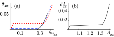
Figure 1: (a): Soft (full line) and semi-soft (dashed and dotted lines) stress-strain curves at $\tilde{r}=0.08$ with $\tilde{h}=0,~{}0.8\tilde{h}_{c},~{}4\tilde{h}_{c}$, respectively. (b) Semi-soft curve of $\tilde{\sigma_{xx}}^{I}$ as a function of $\Lambda_{xx}$ at $\tilde{r}=0.08$ and $\tilde{h}=2\tilde{h}_{c}$, where we have set $v=w$.

The purpose of this paper is to clarify the nature of semi-soft response. We consider the simplest or minimal model, which is formally equivalent to the Maier-Saupe-de-Gennes model deGennesPro1994 for nematic liquid crystals, that exhibits this response. We derive the global mean-field phase diagram [Fig. 2] for this model. We show that semi-soft response is associated with biaxial phases that spontaneously break rotational symmetry, and we unambiguously establish that semi-soft response exists well into the supercritical regime. Figure 1 shows calculated stress-strain curves for $h=0.8h_{c}$ and $h=4h_{c}$ that clearly exhibit semi-soft behavior both for $h<h_{c}$ and in the supercritical regime with $h>h_{c}$. Our minimal model provides a robust description of semi-soft response. We will, however, briefly discuss changes in this response that extensions of the minimal model can bring about.

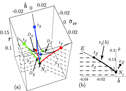
Figure 2: Phase diagrams (a) in the $\tilde{h}$-$\tilde{\sigma}_{xx}$-$\tilde{r}$ space showing the $S_{Y}$ and $S_{Z}$ ($S_{X}$ hidden)$CC$ and the $D_{X}$, $D_{Y}$, and $D_{Z}$ $DC$ surfaces along with the tricritical points $t_{X}$, $t_{Y}$, $t_{Z}$ and (b)in the $\tilde{r}$-$\tilde{h}$ plane ($\tilde{\sigma}_{xx}=0$) showing the first-order uniaxial $PN$-$N$ coexistence line $N_{c}c_{Z}$, the mechanical critical point $c_{Z}$, and the $S_{Z}$ surface terminated by the line $\tilde{r}_{t}(\tilde{h})$ with respective first- and second-order segments $N_{c}t_{Z}$ and $t_{Z}E$ meeting at the tricritical point $t_{Z}$.

An elastomer is characterized by an equilibrium reference configuration, which we refer to as a reference space $S_{R}$, with mass points at positions $\bm{{\rm x}}$. Upon distortion of the elastomer, points $\bm{{\rm x}}$ are mapped to points $\bm{{\rm R}}(\bm{{\rm x}})\equiv\bm{{\rm x}}+\bm{{\rm u}}(\bm{{\rm x}})$ in a target space $S_{T}$, where $\bm{{\rm u}}(\bm{{\rm x}})$ is the displacement variable. Elastic distortions that vary slowly on scales set by the distance between crosslinks are described by the Cauchy deformation tensor $\bm{\Lambda}$ with components $\Lambda_{ij}=\partial R_{i}/\partial x_{j}$. The usual Lagrangian strain tensor is then $\bm{u}=(\bm{\Lambda}^{T}\cdot\bm{\Lambda}-\bm{\delta})/2$, where $\bm{\delta}$ is the unit matrix. The orientational properties of nematic mesogens in the elastomer are measured by the Maier-Saupe nematic tensor $\bm{Q}$.

A complete theory for nematic elastomers should treat both $\bm{\Lambda}$ and $\bm{Q}$ and couplings between them. However, effective theories, obtained by integrating out $Q_{ij}$, that depend only on $\bm{u}$ provide a full description of the mechanical properties of NEs GolubovicLub1989a ; LubenskyXin2002 . In such theories, strains measure distortions relative to an isotropic reference state, and the elastic free-energy density $f(\bm{u})$ consists of an isotropic part $f_{\text{iso}}(\bm{u})$ and an anisotropic part $f_{\text{ani}}(\bm{u},h)$ arising from the imprinting process KupferFin1991 . Equilibrium in the presence of an external second Piola-Kirchhoff (PK) stress $\sigma_{xx}$ is determined by minimization over $\bm{u}$ of the Gibbs free energy density $g(\bm{u},h,\sigma_{xx},r)=f_{\text{iso}}(\bm{u},r)+f_{\text{ani}}(\bm{u},h)+f_{\text{ext}}(\bm{u},\sigma_{xx})$, where $f_{\text{ext}}(\bm{u},\sigma_{xx},)=-\sigma_{xx}u_{xx}$. In equilibrium the second PK stress satisfies $\sigma_{ij}=\partial f/\partial u_{ij}$. We will return later to the engineering or first PK stress tensor $\sigma_{ij}^{I}=\partial f/\partial\Lambda_{ij}=\Lambda_{ik}\sigma_{kj}$.

We now define our minimal model. First, we impose the constraint $\text{Tr}\bm{u}=0$, enforcing incompressibility at small but not large $\bm{u}$, rather than the full nonlinear incompressibility constraint $\det\bm{\Lambda}=[\det(\bm{\delta}+2\bm{u})]^{1/2}=1$ that more correctly describes NEs, whose bulk moduli are generally orders of magnitude larger than their shear moduli. Our theory thus depends only on the symmetric-traceless components of $\bm{u}$: $\phi_{ij}=u_{ij}-\frac{1}{3}\delta_{ij}u_{kk}$, and $f_{\text{ext}}=-\sigma_{xx}\phi_{xx}$. Second , we use the simplest anisotropy energy: $f_{\text{ani}}=-hu_{zz}\rightarrow-h\phi_{zz}$ that favors stretching along the $z$ axis. Thus, our theory is formally equivalent to that for a nematic liquid crystal in crossed electric and magnetic fields, ${\bm{{\rm E}}}=E\bm{{\rm e}}_{z}$ and ${\bm{{\rm H}}}=H\bm{{\rm e}}_{x}$, in which $\phi_{ij}\leftrightarrow Q_{ij}$, $h\leftrightarrow\frac{1}{2}{\Delta\epsilon}E^{2}$, and $\sigma_{xx}\leftrightarrow\frac{1}{2}\chi_{a}H^{2}$, where $\Delta\epsilon$ and $\chi_{a}$ are, respectively, the anisotropic parts of the dielectric tensor and the magnetic susceptibility, and $\bm{{\rm e}}_{a}$, $a=x,y,z$, are unit vectors along direction $a$. Finally, we choose the Landau-de-Gennes form deGennesPro1994 for $f_{\text{iso}}$:

$$f_{\text{iso}}(\bm{\phi},r)=\frac{1}{2}r\text{Tr}\bm{\phi}^{2}-w\text{Tr}\bm{\phi}^{3}+v(\text{Tr}\bm{\phi}^{2})^{2},$$ (1)

where we assume $w>0$ and where $r=a(T-T^{*})$ with $T$ the temperature and $T^{*}$ the temperature at the metastability limit of the $PN$ phase. In the isotropic phase with $\bm{\phi}=0$, $r=2\mu$, where $\mu$ is the $T$-dependent shear modulus. We will often express quantities in reduced form: $\tilde{u}_{ij}=(v/w)u_{ij}$, ${\tilde{r}}=rv/w^{2}$, ${\tilde{h}}=hv^{2}/w^{3}$, $\tilde{\sigma}_{ij}=\sigma_{ij}v^{2}/w^{3}$, $\tilde{C}_{5}=C_{5}v/w^{2}$, and similarly for other elastic moduli.

We begin our analysis of the global phase diagram FriBerPal1987 with the $\sigma_{xx}=0$ plane, which we will refer to as the $Z$-plane because the anisotropy field $h$ favors uniaxial order along the $z$-axis. The $h\geq 0$ half of this plane exhibits the familiar nematic clearing point $N_{c}$ at $(\tilde{r}_{N},\tilde{h}_{N})=(\frac{1}{12},0)$ and the $PN$-$N$ coexistence line terminating at the mechanical critical point $(\tilde{r}_{c},\tilde{h}_{c})=(\frac{1}{8},\frac{1}{192})$. Throughout the $h>0$ half-plane, there is prolate uniaxial order with $\phi_{ij}=S(n_{i}n_{j}-\frac{1}{3}\delta_{ij})$ with $S>0$ and the Frank director $\bm{{\rm n}}$ along $\bm{{\rm e}}_{z}$. In the $N$ phase at $h=0$ and $r<r_{N}$, $\bm{{\rm n}}$ can point anywhere on the unit sphere. Negative $h$ induces oblate rather than prolate uniaxial order along $\bm{{\rm e}}_{z}$ and $S=-S^{\prime}<0$ at high temperature. When $h<0$ is turned on for $r<r_{N}$ at which nematic order exists at $h=0$, $\bm{{\rm n}}$ aligns in the two-dimensional $xy$-plane. This creates a biaxial environment and biaxial rather than uniaxial order. Since $\bm{{\rm n}}$ can point anywhere in the $xy$-plane, the biaxial state at $h<0$ exhibits a spontaneously broken symmetry. There must be a transition along a line $r=r_{t}(h)$ between the high-temperature oblate uniaxial state and the low-temperature biaxial state, which exists throughout the $S_{Z}$ surface shown in Fig. 2. This transition is first order at small $|h|$ because the $PN$-$N$ transition is first order at $h=0$ and second order at larger $|h|$, and there is a tricritical point VargaSza2000 $t_{Z}$ at $(\tilde{r}_{t},\tilde{h}_{t})=(\frac{21}{128},-\frac{27}{1024})$ separating the two behaviors as shown in Fig. 2(b). A continuum of biaxial states coexist on $S_{Z}$. We will refer to such surfaces as $CC$ surfaces and ones on which a discrete set of states coexist as $DC$ surfaces.

The full phase diagram reflects the symmetries of $g$. The $x$- and $z$-directions are equivalent in $f_{\text{iso}}$, and the $\sigma_{xx}=0$ and the $h=0$ planes are symmetry equivalent. These planes are also equivalent (apart from stretching) to the vertical plane with $\sigma_{xx}=h$, but with positive and negative directions interchanged. To see this, we note that $\phi_{zz}+\phi_{xx}=-\phi_{yy}$ and $h\phi_{zz}+\sigma_{xx}\phi_{xx}=-h\phi_{yy}$ when $h=\sigma_{xx}$. Thus the phase structure of the $Z$-plane is replicated in the $X$-plane ($h=0$) and the $Y$-plane ($\sigma_{xx}=h$) with respective preferred uniaxial order along $\bm{{\rm e}}_{x}$ and $\bm{{\rm e}}_{y}$, critical points $c_{X}$ and $c_{Y}$, biaxial coexistence surfaces $S_{X}$ and $S_{Y}$, and tricritical points $t_{X}$ and $t_{Y}$.

To fill in the $3D$ phase diagram, we consider perturbations away from the $X$-, $Y$-, and $Z$-planes. Turning on $\sigma_{xx}$ converts the $PN$-$N$ coexistence line into a $DC$ surface $D_{Z}$, on which two discrete in general biaxial phases coexist. Turning on $\sigma_{xx}$ near the $S_{Z}$ surface favors alignment of the biaxial order along $\bm{{\rm e}}_{x}$ when $\sigma_{xx}>0$ and along $\bm{{\rm e}}_{y}$ when $\sigma_{xx}<0$. Thus $\sigma_{xx}$ is an ordering field for biaxial order whereas a linear combination of $h$ and $\sigma_{xx}$ acts as a nonordering field. The topology of the phase diagram near $t_{Z}$ is that of the Blume-Emery-Griffiths model BluGri1971 with $DC$ surfaces $D_{X}$ and $D_{Y}$ emerging from the first-order line $N_{c}t_{Z}$ terminating $S_{Z}$. The $D_{X}$ and $D_{Y}$ surfaces terminate, respectively, on the critical lines $N_{c}t_{X}$ and $N_{c}t_{Y}$ in the $X$- and $Y$-planes. The surfaces $D_{X}$, $D_{Y}$, and $D_{Z}$ form a cone with vertex at $N_{c}$.

Before considering the $\sigma_{xx}$-$u_{xx}$ stress-strain curve, it is useful to look more closely at elastic response in the vicinity of the $Z$-plane and the nature of order in the $Y$-plane. Throughout the $h>0$ $Z$-plane, the equilibrium state is prolate uniaxial with order parameter $S=S_{0}$, and thus strains $u_{zz}^{0}=\frac{2}{3}S_{0}=-2u_{xx}^{0}=-2u_{yy}^{0}$. We are primarily interested in shears in the $xz$-plane and the response to an imposed $\sigma_{xx}$ with no additional stress along $z$. In this case $\delta u_{zz}=u_{zz}-u_{zz}^{0}$ will relax to an imposed $\delta u_{xx}$, and the free energy of harmonic deviations from equilibrium can be written as $\delta f=\frac{1}{2}C_{3}(\delta u_{xx})^{2}+\frac{1}{2}C_{5}(\delta u_{xz})^{2}$. The modulus $C_{3}$ gives the slope of $\sigma_{xx}$ versus $\delta u_{xx}$, and $C_{5}$ is measured in linearized rheology experiments RogezMar2006 ; terentjev&Co_2003 . $C_{3}$ and $C_{5}$ are easily calculated as a function of $r$ and $h$. In reduced units, the ordered pair $(\tilde{C}_{3},\tilde{C}_{5})$ takes on the value $(\frac{1}{8},\frac{1}{6})$ just above $N_{c}$ ($\tilde{r}=\tilde{r}_{N}^{+}$), $(\frac{3}{8},0)$ just below $N_{c}$ ($\tilde{r}=\tilde{r}_{N}^{-}$), $(0,\frac{1}{12})$ at the critical point, and $(\frac{57}{112},\frac{1}{12})$ in the supercritical regime at $(\tilde{r},\tilde{h})=(\tilde{r}_{c},2\tilde{h}_{c})$. We will measure elastic distortions using $\delta u_{ij}$ rather than the strain $u^{\prime}_{ij}$ relative to the reference space $S^{\prime}_{R}$ defined by the equilibrium configuration at any given $T$ u' .

On the $h>0$, $Y$-plane, there is oblate uniaxial order aligned along the $y$-direction at high $T$ and biaxial order at low $T$. A convenient representation of the tensor order parameter is

$$\bm{\phi}=\left(\begin{array}[]{ccc}\frac{1}{3}S^{\prime}-\eta_{1}&0&\eta_{2}\\ 0&-\frac{2}{3}S^{\prime}&0\\ \eta_{2}&0&\frac{1}{3}S^{\prime}+\eta_{1}\end{array}\right),$$ (2)

where $S^{\prime}>0$. The vector $\vec{\eta}\equiv(\eta_{1},\eta_{2})\equiv\eta(\cos 2\theta,\sin 2\theta)$ is the biaxial order parameter, which is nonzero on the $S_{Y}$ surface. We define the equilibrium values of $S^{\prime}$ and $\eta$ in the biaxial phase to be $S_{0}^{\prime}$ and $\eta_{0}$, respectively. Energy in this phase is independent of the rotation angle $\theta$. Away from the $Y$-plane, $f_{\text{ani}}+f_{\text{ext}}=-\frac{1}{3}(h+\sigma_{xx})S^{\prime}+(\sigma_{xx}-h)\eta_{1}$. Thus, $\sigma_{xx}<h$ favors $\eta_{1}>0$ and $\sigma_{xx}>h$ favors $\eta_{1}<0$, implying that $\vec{\eta}=(\eta_{0},0)$ (or $\theta=0$) at $\sigma_{xx}=h^{-}$ and $\vec{\eta}=(-\eta_{0},0)$ (or $\theta=\frac{\pi}{2}$) at $\sigma_{xx}=h^{+}$. These considerations imply that the modulus $C_{5}$ is zero at $\sigma_{xx}=h^{\pm}$ because $C_{5}=\partial^{2}f/\partial u_{xz}^{2}|_{u_{xz}\rightarrow 0}=(2\eta_{0})^{-2}\partial^{2}f/\partial\theta^{2}|_{\theta\rightarrow 0}=0$.

We can now construct the $\sigma_{xx}$-$u_{xx}$ stress-strain curves. At $\sigma_{xx}=0$, $u_{xx}=u_{xx}^{0}$; as $\sigma_{xx}$ is increased from zero, $\delta u_{xx}$ grows with initial slope $1/C_{3}$ until $\sigma_{xx}=h^{-}$ at which point, $\delta u_{xx}=\frac{1}{3}S^{\prime}_{0}-u_{xx}^{0}-\eta_{0}$. At $\sigma_{xx}=h$, further increase of $\delta u_{xx}$ to a maximum of $\frac{1}{3}S^{\prime}_{0}-u_{xx}^{0}+\eta_{0}$ produces a zero-energy rotation of $\vec{\eta}$ to yield $\delta u_{xx}=\frac{1}{3}S^{\prime}_{0}-u_{xx}^{0}-\eta_{0}\cos 2\theta$ and a nonzero shear $u_{xz}=\eta_{2}=\eta_{0}\sin 2\theta$. The growth of $\eta_{2}$ from zero is induced by the vanishing of $C_{5}$ at $\sigma_{xx}=h^{\pm}$ and its becoming negative for $|\eta_{1}|<\eta_{0}$. Thus, the characteristic semi-soft plateau is a consequence of $C_{5}$’s vanishing at $\sigma_{xx}=h$ and not at $\sigma_{xx}=0$. Measurements of $C_{5}$ at $\sigma_{xx}=0$ do not provide information about what happens at $\sigma_{xx}=h$. For $\sigma_{xx}>h$, $\delta u_{xx}$ again grows with $\sigma_{xx}$. Figure 1 shows stress-strain curves for different values of $\tilde{h}$. Thus, semi-soft response is associated with the $S_{Y}$ surface, which exists at $r$ and $h$ well into the supercritical regime.

A Ward identity provides a rigorous basis for the above picture beyond mean-field theory. $f_{\text{iso}}(\bm{u})$ is invariant under rotations of $\bm{u}$, i.e., under $\bm{u}\rightarrow\bm{U}\bm{u}\bm{U}^{-1}$ where $\bm{U}$ is any rotation matrix. Thus if $f_{\text{ani}}=-\text{Tr}\bm{h}\bm{u}$, where $h_{ij}=he_{zi}e_{zj}$, $f(\bm{U}\bm{u}\bm{U}^{-1})=f_{\text{iso}}(\bm{u})-\text{Tr}\bm{h}\bm{U}\bm{u}\bm{U}^{-1}$, for any $\bm{U}$, including one describing an infinitesimal rotation by $\gamma$ about the $y$-axis with components $U_{ij}=\delta_{ij}+\epsilon_{yij}\gamma$, where $\epsilon_{ijk}$ is the Levi-Civita anti-symmetric tensor. Equating the term linear in $\gamma$ in $f(\bm{U}\bm{u}\bm{U}^{-1})$ to that of $\text{Tr}\bm{h}\bm{U}\bm{u}\bm{U}^{-1}$ yields the Ward identity

$$\sigma_{xz}(u_{zz}-u_{xx})=(\sigma_{zz}+h-\sigma_{xx})u_{xz},$$ (3)

where $\sigma_{ij}=\partial f/\partial u_{ij}$. This identity applies for any $f_{\text{iso}}$, including ones with no compressibility constraint, so long as $f_{\text{ani}}$ is linear in $\bm{u}$. In the semi-soft geometry $\sigma_{xz}=\sigma_{zz}=0$ but $\sigma_{xx}>0$. Thus, either $u_{xz}=0$ or $\sigma_{xx}=h$ for any nonzero $u_{xz}$. Equation (3) also gives $C_{5}=\sigma_{xz}/u_{xz}|_{u_{xz}\rightarrow 0}=(h-\sigma_{xx})/(u_{zz}-u_{xx})=|h-\sigma_{xx}|/2\eta_{0}$ implying that $C_{5}\rightarrow 0$ as $\sigma_{xx}\rightarrow h^{\pm}$ as long as $\eta_{0}\neq 0$.

We have focussed on the effects of an external second PK stress $\sigma_{xx}$. In physical experiments, the first PK (engineering) stress, $\sigma_{ij}^{I}=\partial f/\partial\Lambda_{ij}=\Lambda_{ik}\sigma_{kj}$, or the Cauchy stress, $\sigma_{ij}^{C}=\sigma_{ik}^{I}\Lambda_{kj}^{T}/\det\bm{\Lambda}$ (as in WarnerTer2003 ; Warner1999 ), is externally controlled. The $\sigma_{xx}^{I}$-$\Lambda_{xx}$ stress-strain curve is easily obtained from the $\sigma_{xx}$-$u_{xx}$ curve using $\sigma_{xx}^{I}=\Lambda_{xx}\sigma_{xx}$ and $\Lambda_{xx}=\sqrt{1+2u_{xx}}$. These two curves are similar, but the flat plateau in the $\sigma_{xx}^{I}$-$\Lambda_{xx}$ curve rises linearly with $\Lambda_{xx}$ as shown in Fig. 1(b), and there is a unique value of $\Lambda_{xx}$ for each value of $\sigma_{xx}^{I}$. Thus, the $S_{Y}$ surface in the $r$-$h$-$\sigma_{xx}$ phase diagram would open into a finite volume biaxial region in the $r$-$h$-$\sigma_{xx}^{I}$ phase diagram with a particular value of $\vec{\eta}$ at each point in it. The phase diagram in the $h$-$\sigma_{xx}^{I}$ plane for $r_{c}<r<r_{t}$ is similar to that in Fig. 3(b).

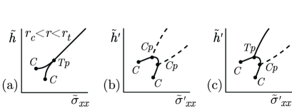
Figure 3: Schematic phase diagrams in the $h$(or $h^{\prime}$)-stress plane. The points $Tp$, $C$ and $Cp$ are, respectively, triple points, liquid-gas-like critical points, and critical endpoints. (a) Diagrams for the minimal model, where all transitions are first order; (b) and (c) Phase diagrams for more general $f_{\text{ani}}$ or $f_{\text{ext}}$ in which the first-order line from $S_{Y}$ is replaced by a surface terminated by two second-order (dashed) lines or one first-order line and one second-order line. $h^{\prime}$ and $\sigma^{\prime}_{xx}$ are, respectively, the generalized aligning field and generalized external stress resulting from the more general $f_{\text{ani}}$ or $f_{\text{ext}}$.

We have ignored boundary conditions and random stress, both of which can modify stress-strain curves. When Frank elastic energies are ignored, detailed calculations of domain structure induced by boundary conditions reproduce soft and semi-soft response ContiDol2002a . Small isotropic randomness appears not to affect soft response, but large randomness does Uchida2000 . Our approach should serve as a basis for further study of randomness.

We can now consider modifications of the minimal model. A simple modification is to replace the constraint $\text{Tr}\bm{u}=0$ with the real volume constraint $\det\bm{\Lambda}=1$. This replacement does not change the validity of the Ward identity and the resulting phase diagram has the same structure as that for $\text{Tr}\bm{u}=0$ but with different boundaries for the $CC$ and $DC$ surfaces. In particular, the mechanical critical point is at $(\tilde{r}_{c},\tilde{h}_{c})=(0.1279,0.0052)$ and the tricritical point is at $(\tilde{r}_{t},\tilde{h}_{t})=(0.1900,0.0247)$. Other modifications of the minimal model replace $f_{\text{ani}}$ with nonlinear functions of $u_{zz}$. Modifications of this kind can spread the $CC$ surface $S_{Y}$ into a finite volume or convert it to a $DC$ surface, as shown in Fig. 3. If $f_{\text{ani}}=-hu_{zz}^{2}$, two states coexist, whereas with other forms such as might arise in a hexagonal lattice, three or more discrete states might coexist. When $S_{Y}$ is a $DC$ surface, rather than exhibiting a homogeneous rotation of the biaxial order parameter (if boundary conditions are ignored) in response to an imposed $u_{xx}$, samples will break up into disrete domains of the allowed states. In other words, their response to external stress will be martensitic Bhattacharya2003 rather than semi-soft.

The neo-classical model BlandonWar1994 can also be discussed in our language. The free energy of this model is a function of $\bm{\Lambda}$ and $\bm{Q}$. It consists of an isotropic part, invariant under simultaneous rotations of $\bm{\Lambda}$ and $\bm{Q}$ in the target space and under rotations of $\bm{\Lambda}$ in the reference space, and a semi-soft anisotropic energy VerwayWar1995 , which is effectively nonlinear in the strain, that breaks rotational symmetry in the reference space. The phase diagram of this model is similar to that of the minimal model in the space of $r$-$h$-$\sigma_{xx}^{I}$. In it, semi-soft behavior also persists above the mechanical critical point YeLub2007 .

In summary, we determined the complete phase diagram of nematic elastomers subject to an internal aligning field and a perpendicular external stress. Our results underscore the validity of semi-softness in the interpretation of their remarkable stress-strain curves.

This work was supported by NSF grant DMR 0404570 and the NSF MRSEC under DMR 05-20020.

References

- (1) M. Warner and E. M. Terentjev, Liquid Crystal Elastomers (Oxford University Press, Oxford, 2003).
- (2) M. Warner, P. Bladon, and E. M. Terentjev, J. Phys. II (France) 4, 93 (1994).
- (3) P. D. Olmsted, J. Phys. II (France) 4, 2215 (1994).
- (4) L. Golubović and T. C. Lubensky, Phys. Rev. Lett. 63, 1082 (1989).
- (5) J. Küpfer and H. Finkelmann, Makromol. Chem. Rapid Commun. 12, 717 (1991).
- (6) G. Verway and M. Warner, Macromolecules 28, 4303 (1995).
- (7) J. Küpfer and H. Finkelmann, Macromol. Chem. Phys. 195, 1353 (1994).
- (8) M. Warner, J. Mech. Phys. of Solids 47, 1355 (1999).
- (9) O. Stenull and T. C. Lubensky, Eur. Phys. J. E 14, 333 (2004).
- (10) P. de Gennes, C.R. Acad. Sci. Ser. B 281, 101 (1975).
- (11) A. Lebar et al., Phys. Rev. Lett. 94, 197801 (2005).
- (12) D. Rogez et al., Eur. Phys. J. E 20, 369 (2006).
- (13) H. R. Brand, H. Pleiner, and P. Martinoty, Soft Matter 2, 182 (2006).
- (14) P. de Gennes and J. Prost, The Physics of Liquid Crystals (Oxford University Press, Oxford, 1993).
- (15) T. C. Lubensky et al., Phys. Rev. E 66, 031704 (2002).
- (16) B. J. Frisken, B. Bergersen, and P. Palffy-Muhoray, Mol. Cryst. Liq. Cryst. 148, 45 (1987).
- (17) C.-P. Fan and M. J. Stephen, Phys. Rev. Lett. 25, 500 (1970); R. G. Priest, Phys. Lett. 47A, 475 (1974).
- (18) M. Blume, V. Emery, and R. Griffiths, Phys. Rev. A 4, 1071 (1971).
- (19) A. Hotta and EṀ. Terentjev, Eur. Phys. J. E 10, 291 (2003); E. M. Terentjev, et al., Phil. Trans. R. Soc. Lond. A 361, 653 (2003).
- (20) The deformation tensor of the anisotropic equilibrium state at temperature relative to is . The strain and stress relative to are, respectively, and .
- (21) S. Conti, A. DeSimone, and G. Dolzmann, J. Mech. Phys. of Solids 50, 1431 (2002); Phys. Rev. E 66, 061710 (2002).
- (22) N. Uchida, Phys. Rev. E 62, 5119 (2000).
- (23) K. Bhattacharya, Microstructure of Martensite (Oxford University Press, New York, 2003).
- (24) P. Blandon, E. Terentjev, and M. Warner, J. Phys. II (France) 4, 75 (1994).
- (25) F. Ye and T. C. Lubensky (unpublished).