Relation between exchange-only optimized potential and Kohn-Sham methods with finite basis sets; solution of a paradox

Abstract

Arguments showing that exchange-only optimized effective potential (xOEP) methods, with finite basis sets, cannot in general yield the Hartree-Fock (HF) ground state energy, but a higher one, are given. While the orbital products of a complete basis are linearly dependent, the HF ground state energy can only be obtained via a basis set xOEP scheme in the special case that all products of occupied and unoccupied orbitals emerging from the employed orbital basis set are linearly independent from each other. In this case, however, exchange potentials leading to the HF ground state energy exhibit unphysical oscillations and do not represent a Kohn-Sham (KS) exchange potential. These findings solve the seemingly paradoxical results of Staroverov, Scuseria and Davidson that certain finite basis set xOEP calculations lead to the HF ground state energy despite the fact that within a real space (or complete basis) representation the xOEP ground state energy is always higher than the HF energy. Moreover, whether or not the occupied and unoccupied orbital products are linearly independent, it is shown that basis set xOEP methods only represent exact exchange-only (EXX) KS methods, i.e., proper density-functional methods, if the orbital basis set and the auxiliary basis set representing the exchange potential are balanced to each other, i.e., if the orbital basis is comprehensive enough for a given auxiliary basis. Otherwise xOEP methods do not represent EXX KS methods and yield unphysical exchange potentials. The question whether a xOEP method properly represents a KS method with an exchange potential that is a functional derivative of the exchange energy is related to the problem of the definition of local multiplicative operators in finite basis representations and to the fact that the Hohenberg Kohn theorem does not apply in finite basis representations. Plane wave calculations for bulk silicon illustrate the findings of this work.

I Introduction

In a recent stimulating article with important implications for the use of finite basis sets, Staroverov, Scuseria, and Davidson staroverov06 presented an exchange-only optimized effective potential (xOEP) scheme that yields, for given finite Gaussian orbital basis sets, ground state energies that surprisingly equal exactly the ground state Hartree-Fock (HF) energies for these basis sets. Moreover, their xOEP scheme not only yields one unique but an infinite number of exchange potentials and each of the latter leads to the corresponding ground state HF energy if used as the exchange potential in the corresponding exchange-only KS Hamiltonian operator. On the other hand, it is known that in a complete basis set limit, which corresponds to a complete real space representation of all quantities, the xOEP method is identical sahni82 to the exact exchange-only Kohn-Sham method and yields ground state energies that always lie above ivanov03 the corresponding ground state HF energy. Staroverov, Scuseria, and Davidson then state: ”Our conclusions may appear paradoxical. For any finite basis set, no matter how large, there exist infinitely many xOEP’s that deliver exactly the ground-state HF energy in that basis, however close it may be to the HF limit. Nonetheless, in the complete basis set limit, the xOEP is unique and E(xOEP) is above E(HF)”. (Here E(xOEP) and E(HF) denote the xOEP and HF total energies, respectively, that are denoted $E^{xOEP}$ and $E^{HF}$ in this work.) Furthermore they state: ”The non-uniqueness of OEPs in a finite basis set raises doubt about their usefulness in practical applications”

We here first show, by different means including a constrained-search one, that the above statement of Staroverov, Scuseria, and Davidson, that it is always possible to construct optimized effective potentials that deliver exactly the ground state HF energy, holds if and only if the products of the orbital basis functions, or at least the products of the corresponding occupied and unoccupied HF orbitals from a given orbital basis set, form a linearly independent set. Otherwise, the xOEP scheme for finite orbital basis sets, in general, does not deliver exactly the ground state HF energy. Secondly, we show that the xOEP approach of Staroverov, Scuseria, and Davidson, does not really represent an exchange-only KS method and does not yield physically meaningfull KS exchange potentials, even if the products of orbital basis functions are linearly independent. In order to get physically meaningfull KS exchange potentials via xOEP schemes, the latter have to be set up in a way that they represent KS methods, otherwise they are indeed of little usefulness in practical applications. However, if xOEP schemes are set up properly then they are of great usefulness in practice as demonstrated, e.g., by numerically stable plane-wave xOEP procedures for solids stadele97 ; stadele99 ; magyar04 ; qteish05 ; rinke05 .

II Relation of xOEP and HF energies within finite basis set methods

We start by briefly reconsidering the xOEP approach of Staroverov, Scuseria, and Davidson staroverov06 . The relevant Hamiltonian operators are the HF Hamiltonian operator

$$\hat{H}^{HF} = -{\textstyle\frac{1}{2}}\nabla^{2}+{v}_{ext}({\bf r})+{v}_{H}({\bf r})+\hat{v}_{x}^{NL}$$ (1)

and the exchange-only KS Hamiltonian operator

$$\hat{H}^{xKS} = -{\textstyle\frac{1}{2}}\nabla^{2}+{v}_{s}({\bf r})$$ (2)

$$= -{\textstyle\frac{1}{2}}\nabla^{2}+{v}_{ext}({\bf r})+{v}_{H}({\bf r})+{v}_{x}({\bf r})$$

Atomic units are used throughout. In Eqs. (1) and (2), ${v}_{ext}({\bf r})$ denotes the external potential, usually the electrostatic potential of the nuclei, ${v}_{H}({\bf r})$ is the Hartree potential, i.e., the Coulomb potential of the electron density, ${v}_{x}({\bf r})$ is the local multiplicative KS exchange potential, ${v}_{s}({\bf r})={v}_{H}({\bf r})+{v}_{x}({\bf r})+{v}_{ext}({\bf r})$ the effective KS potential, and $\hat{v}_{x}^{NL}$ the nonlocal exchange operator with the kernel

$$\hat{v}_{x}^{NL}({\bf r},{\bf r}^{\prime}) = \frac{\rho({\bf r},{\bf r}^{\prime})}{|{\bf r}-{\bf r}^{\prime}|}$$ (3)

in a real space representation. Here $\rho({\bf r},{\bf r}^{\prime})$ designates the first-order density matrix. In the HF-Hamiltonian operator of Eq. (1) the first-order density matrix occuring in the nonlocal exchange operator of Eq. (3) equals the HF first order density matrix $\rho^{HF}({\bf r},{\bf r}^{\prime})$ and the nonlocal exchange operator subsequently equals the HF exchange operator. For simplicity we consider closed shell systems with non-degenerate ground states. In this case orbitals, first-order density matrices, and basis functions can all be chosen to be real-valued.

Next we introduce an orbital basis set $\{\chi_{\mu}\}$ of dimension $N$. The representations of the HF- and exchange-only KS-Hamiltonian operators in this basis set are

$${\bf H}^{HF} = {\bf T}+{\bf V}_{H}+{\bf V}_{x}^{NL}+{\bf V}_{ext}$$ (4)

and

$${\bf H}^{xKS} = {\bf T}+{\bf V}_{s}$$ (5)

$$= {\bf T}+{\bf V}_{H}+{\bf V}_{x}+{\bf V}_{ext}\,,$$

respectively. The matrices ${\bf T}$, ${\bf V}_{H}$, ${\bf V}_{ext}$, ${\bf V}_{x}^{NL}$ and ${\bf V}_{x}$ are defined by the corresponding matrix elements $T_{\mu\nu}=\langle\chi_{\mu}|-{\textstyle\frac{1}{2}}\nabla^{2}|\chi_{\nu}\rangle$, $V_{H,\mu\nu}=\langle\chi_{\mu}|{v}_{H}|\chi_{\nu}\rangle$, $V_{ext,\mu\nu}=\langle\chi_{\mu}|{v}_{ext}|\chi_{\nu}\rangle$, $V_{x,\mu\nu}^{NL}=\langle\chi_{\mu}|\hat{v}_{x}^{NL}|\chi_{\nu}\rangle$, and $V_{x,\mu\nu}=\langle\chi_{\mu}|\hat{v}_{x}|\chi_{\nu}\rangle$, respectively, and by ${\bf V}_{s}={\bf V}_{H}+{\bf V}_{x}+{\bf V}_{ext}$. Because the orbital basis functions are real-valued all matrices are symmetric

Now we expand the KS exchange potential in an auxiliary basis set $\{f_{k}\}$ of dimension $M^{aux}$, i.e.,

$${v}_{x}({\bf r})=\sum_{k=1}^{M^{aux}}\;b_{k}\,f_{k}({\bf r})\,.$$ (6)

The auxiliary basis set, of course, shall be chosen such that its basis functions are linearly independent. The crucial question arising now is how many and what types of matrices ${\bf V}_{x}$ representing the KS density-functional exchange potential can be constructed for a given auxiliary basis set $\{f_{k}\}$. This question was answered in Ref. [gorling95, ]. Firstly we consider the case when the $M=(1/2)N(N+1)$ different products $\chi_{\mu}({\bf r})\chi_{\nu}({\bf r})$ of orbital basis functions are linearly independent. In this case, if $M^{aux}=M$ and the auxiliary basis functions span the same space as the products of the orbital basis functions, then a symmetric matrix ${\bf V}_{x}$ can be constructed in a unique way by determining appropriate expansion coefficients $b_{k}$ for the exchange potential. The reason is that the determination of the $M^{aux}=M$ expansion coefficients $b_{k}$ for the construction of the $M^{aux}=M$ different matrix elements of the symmetric matrix ${\bf V}_{x}$ leads to a linear system of equations

$${\bf A}\,{\bf b}={\bf W}_{x}$$ (7)

with

$${A}_{\mu\nu,t}=\langle\chi_{\mu}\chi_{\nu}|f_{k}\rangle$$ (8)

for the coefficients $b_{k}$ of dimension $M^{aux}=M$ that is nonsingular and thus has a unique solution gorling95 . In Eq.  (7), ${\bf A}$ is a $M\times M^{aux}$ matrix that contains the overlap matrix elements $\langle\chi_{\mu}\chi_{\nu}|f_{k}\rangle$. The first index of ${\bf A}$, i.e., $\mu\nu$, is a superindex refering to products of orbital basis functions while the second index, $k$, refers to auxiliary basis functions. The vector ${\bf b}$ collects the expansion coefficients of Eq. (6) for the exchange potential and the right hand side ${\bf W}_{x}$, a vector with superindices $\mu\nu$, contains the $M=N(N+1)/2$ independent elements of an arbitrarily chosen matrix ${\bf V}_{x}$. If we chose ${\bf V}_{x}$ to be equal to the matrix representation of an arbitrary nonlocal operator with respect to the orbital basis set then Eqs. (6) and (7) define a local potential with the same matrix representation. This demonstrates that a distinction of local multiplicative and nonlocal operators is not clearly possible for orbital basis sets with linearly independent products of orbital basis functions.

If $M^{aux}>M$ and the space spanned by the auxiliary functions contains the space spanned by the product of orbital functions then gorling95 an infinite number of sets of coefficients $b_{k}$ lead to any given symmetric matrix ${\bf V}_{x}$. The real space KS exchange potentials ${v}_{x}({\bf r})$ corresponding according to Eq. (6) to these sets of coefficients $b_{k}$ are all different but all represent local multiplicative potentials. Next we construct KS Hamiltonian operators (2) by adding these different KS exchange potentials to always the same external and Hartree potential. The resulting effective KS potentials in real space, i.e., the ${v}_{s}({\bf r})$ are all different. Nevertheless the resulting basis set representations ${\bf H}^{xKS}$ of the corresponding KS Hamiltonian operators are all identical because the basis set representations ${\bf V}_{x}$ of the different exchange potentials ${v}_{x}({\bf r})$, by construction, are all identical. As a consequence the KS orbitals resulting from diagonalizing the KS Hamiltonian matrix ${\bf H}^{xKS}$ and subsequently also the resulting ground state electron densities are identical in all cases. We thus have a situation where different local multiplicative KS potentials ${v}_{s}({\bf r})$ lead to the same ground state electron density. This seems to constitute a violation of the Hohenberg-Kohn theorem. Indeed it was shown in Ref. [harriman86, ] and discussed in Ref. [gorling95, ] that the Hohenberg-Kohn theorem does not hold for finite orbital basis sets in its original formulation, i.e., that different local potentials, e.g., local potentials obtained by different linear combinations of auxiliary basis funtions, must lead to different KS determinants and thus different KS electron densities. We will come back to this point later on. Finally, if $M^{aux}<M$ then not all symmetric matrices ${\bf V}_{x}$ can be constructed from a local KS exchange potential given by an expansion (6).

In their xOEP approach Staroverov, Scuseria, and Davidson staroverov06 can expand the KS exchange potential in $M^{aux}=M$ auxiliary basis functions and determine the coefficients such that the resulting matrix ${\bf V}_{x}$ exactly equals the HF exchange matrix ${\bf V}_{x}^{NL}$. If additionally the KS Hartree potential is set equal to the HF one then the resulting HF and KS Hamiltonian operators are identical. Subsequently also the HF and KS orbitals, the ground state electron densities, and the ground state energies are identical. Because the HF and the KS electron densities turn out to be identical, the Coulomb potential of this density can equally well be considered as a HF or a KS Hartree potential. It follows immediately that the KS exchange potential constructed in this way is the xOEP exchange potential: The HF total energy is the lowest total energy any Slater determinant can yield. Thus if a local multiplicative KS potential leads to this total energy it is clearly the optimized effective potential defined as the potential that yields the lowest total energy achievable by any local multiplicative KS potential. The xOEP ground state energy resulting from this construction equals the corresponding HF energy. Moreover by enlarging the number of auxiliary basis functions, resulting in $M^{aux}>M$, not only one optimized exchange potential leading to the HF energy but infinitely many can be constructed.

Staroverov, Scuseria, and Davidson obtained the HF energy in their xOEP scheme even if the number of auxiliary functions only equaled the product $M^{ov}$ of occupied and virtual orbitals staroverov06 . In this case a similarity transformation of the HF and the KS Hamiltonian matrices and their constituents was carried out in order to obtain representations of all matrices with respect to the HF orbitals. Then it is sufficient to chose the expansion coefficients of the KS exchange potential such that only the occupied-virtual block of the KS exchange matrix equals that of the HF exchange matrix. The resulting KS Hamiltonian matrix then may differ from the HF Hamiltonian matrix in the occupied-occupied and the virtual-virtual block but this merely leads to unitary transformations of the occupied and virtual orbitals among themselves and thus does not change the ground state energy or the electron density.

Indeed it is straightforward to show that the occupied-virtual block of the exchange matrix equals that of the HF exchange matrix if the products of occupied and unoccupied orbitals are linearly independent. To that end we consider the xOEP equation determining the xOEP exchange potential sharp53 ; talman76

$$4\sum_{i}^{occ.}\sum_{a}^{unocc.}\;\phi_{i}({\bf r})\phi_{a}({\bf r})\;\frac{\langle\phi_{a}|v_{x}|\phi_{i}\rangle}{\varepsilon_{i}-\varepsilon_{a}} = 4\sum_{i}^{occ.}\sum_{a}^{unocc.}\;\phi_{i}({\bf r})\phi_{a}({\bf r})\;\frac{\langle\phi_{a}|v_{x}^{NL}|\phi_{i}\rangle}{\varepsilon_{i}-\varepsilon_{a}}\,.$$ (9)

In Eq. (9) $\phi_{i}$ and $\phi_{a}$ denote occupied and unoccupied KS orbitals, respectively, with eigenvalues $\varepsilon_{i}$ and $\varepsilon_{a}$. Both sides of Eq. (9) are a linear combination of products $\phi_{i}({\bf r})\phi_{a}({\bf r})$ of occupied and unoccupied KS orbitals with coefficients ${\langle\phi_{a}|v_{x}|\phi_{i}\rangle}/{(\varepsilon_{i}-\varepsilon_{a})}$ and ${\langle\phi_{a}|v_{x}^{NL}|\phi_{i}\rangle}/{(\varepsilon_{i}-\varepsilon_{a})}$, respectively. However, if the products $\phi_{i}({\bf r})\phi_{a}({\bf r})$ are linearly independent then the two linear combinations can only be identical if the coefficients multiplying the products are all identical. This, however, requires that $\langle\phi_{a}|v_{x}|\phi_{i}\rangle=\langle\phi_{a}|v_{x}^{NL}|\phi_{i}\rangle$, i.e., that the occupied-virtual block of the KS exchange matrix equals that of the corresponding exchange matrix of a nonlocal exchange operator of the form of the HF exchange operator. Replacement of the KS exchange matrix by the matrix of the nonlocal exchange operator thus again leads only to a unitary transformation of the occupied and virtual orbitals among themselves. Therefore the corresponding xOEP determinant can also be interpreted as HF determinant.

Next we consider the crucial point what happens if the products of orbital basis functions $\chi_{\mu}({\bf r})\chi_{\nu}({\bf r})$ are linearly dependent. Then the rows of the matrix ${\bf A}$ of Eq. (7) are linearly dependent, thus the rank of the matrix ${\bf A}$ is lower than $M$, and as consequence Eq. (7), in general, has no solution. For an alternative argument, observe that for linear dependent products of orbital basis functions $\chi_{\mu}({\bf r})\chi_{\nu}({\bf r})$, there exists at least one linear combination of such products that equals zero

$$0=\sum_{\mu\nu}\;a_{\mu\nu}\,\chi_{\mu}({\bf r})\chi_{\nu}({\bf r})\,.$$ (10)

In Eq. (10) the $a_{\mu\nu}$ denote the coefficients of that linear combination. The corresponding sum of matrix elements of ${\bf V}_{x}$ also equals zero, i.e.,

$$0=\sum_{\mu\nu}\;a_{\mu\nu}\,\langle\chi_{\mu}|v_{x}|\chi_{\nu}\rangle=\int\!d{\bf r}\,v_{x}({\bf r})\,\sum_{\mu\nu}\;a_{\mu\nu}\,\chi_{\mu}({\bf r})\chi_{\nu}({\bf r})$$ (11)

for any choice of expansion coefficients $b_{t}$ in Eq. (6) because the product of any local function and thus of any KS exchange potential ${v}_{x}({\bf r})$ with the sum (10) equals zero. The products $\chi_{\mu}({\bf r})\chi_{\nu}({\bf r}^{\prime})$ for two different arguments ${\bf r}$ and ${\bf r}^{\prime}$, on the other hand, are always linearly independent because the orbital basis set $\{\chi_{\mu}\}$ has to be linearly independent. Therefore the linear combination $\sum_{\mu\nu}\;a_{\mu\nu}\,\chi_{\mu}({\bf r})\chi_{\nu}({\bf r}^{\prime})$ can not be identical to zero for all values of the arguments ${\bf r}$ and ${\bf r}^{\prime}$. Then, however, also the integral of this linear combination with $\rho^{HF}({\bf r},{\bf r}^{\prime})/|{\bf r}-{\bf r}^{\prime}|$, i.e., with the kernel of the nonlocal HF exchange operator, in general, is not equal to zero, i.e., in general

$$0\neq\sum_{\mu\nu}\;a_{\mu\nu}\,\langle\chi_{\mu}|\hat{v}_{x}^{HF}|\chi_{\nu}\rangle\,.$$ (12)

Comparison of Eqs. (11) and (12) shows that, in general, the exchange matrices ${\bf V}_{x}$ and ${\bf V}_{x}^{NL}$ are different no matter how the expansion coefficients $b_{k}$ of the KS exchange potential, Eq. (6), are chosen. This demonstrates that, in general, neither the xOEP scheme of Staroverov, Scuseria, and Davidson staroverov06 nor any other leads to an xOEP Hamiltonian operator that equals the HF Hamiltonian operator when the orbital basis products are linearly dependent. If we consider the version of Staroverov, Scuseria, and Davidson’s xOEP scheme that refers only to the occupied-virtual block of the xOEP and HF exchange matrices then by completely analogous arguments it follows that this scheme only works if the products of occupied and unoccupied HF orbitals are linearly independent. However, in general, if the products of occupied and unoccupied HF orbitals are linearly dependent then it is not possible to obtain the HF ground state energy via an xOEP scheme.

II.1 Constrained-search analysis

Before we discuss the question how products of basis functions can become linearly dependent for given orbital basis sets we elucidate the situation from a constrained-search levy79 point of view. We start with a constrained-search proof that the xOEP ground state energy, $E^{xOEP}$, must equal the HF ground state energy, $E^{HF}$, in their common finite orbital basis, when there is no linear dependence in the products of orbital basis functions. To accomplish this we appeal to the work of Harriman harriman86 . He showed that only one first-order density matrix may yield any density generated by a given finite orbital basis whose basis products form a linearly independent set. This means that since an idempotent first-order density matrix uniquely fixes a corresponding single determinant, it follows that only one single determinant, constructed from a given finite orbital basis whose products are linearly independent, may yield a density that is constructed from this same basis. Consequently, with use of a common finite orbital basis set, the xOEP single determinant must equal the HF single determinant if there exists an effective KS potential $v_{s}$ in Eq (2) such that the corresponding KS ground state density is the same as the Hartree-Fock density. That this $v_{s}$ exists for the situation when the basis products are linearly independent, as discussed above, follows from Ref.[gorling95, ] and was shown in practice by Staroverov, Scuseria, and Davidson staroverov06 .

What happens when the products are not linearly independent? Due to the idempotency property of the first-order density matrix for a single determinant, a density generated from a given finite orbital basis could still generate a unique determinant if the basis products are linearly dependent, provided that this linear dependency is mild enough levy87 , i.e., if the products of occupied and unoccupied orbitals remain linearly independent. However, if the linear dependency of the basis product pairs is not sufficiently mild, then the situation changes dramatically in that more than one single determinant will yield the same density from a given finite basis set levy87 . In this case we do not have equality $E^{xOEP}=E^{HF}$. Instead, we have inequality $E^{xOEP}>E^{HF}$, which arises from the following contradiction.

Assume that the xOEP determinant $\Phi^{xOEP}$ equals the HF determinant $\Phi^{HF}$ through respective optimizations in their common finite orbital basis set. Then it follows that their densities must be the same. But, from a constrained-search analysis constrainedsearch , the xOEP determinant $\Phi^{xOEP}$ would yield this HF density and minimize, within this common basis, just the expectation value $\langle\Phi|\hat{T}|\Phi\rangle$ of the kinetic energy, while the HF determinant $\Phi^{HF}$ yields this HF density and minimizes, within the common basis, the expectation value $\langle\Phi|\hat{T}+\hat{V}_{ee}|\Phi\rangle$ of the kinetic energy plus the electron-electron repulsion energy. Here $\hat{T}$ denotes the many-electron kinetic energy operator, $\hat{V}_{ee}$ the corresponding electron-electron repulsion operator, and $\Phi$ Slater determinants that yield the HF density. (Equivalently, the xOEP determinant would yield the HF density and minimize $\langle\Phi|\hat{H}-\hat{V}_{ee}|\Phi\rangle$ while the HF determinant yields this HF density and of course minimizes $\langle\Phi|\hat{H}\Phi\rangle$. Here $\hat{H}$ denotes the many-electron Hamiltonian operator.). Because the Slater determinants $\Phi^{xOEP}$ and $\Phi^{HF}$ minimize different expectation values, i.e., $\langle\Phi|\hat{T}|\Phi\rangle$ and $\langle\Phi|\hat{T}+\hat{V}_{ee}|\Phi\rangle$, respectively, they are different, in general, and the inequality $E^{xOEP}>E^{HF}$ applies for this common finite orbital basis case. However, there is only one possible determinant $\Phi$ that yields the HF density from a given finite basis when the basis products are linearly independent or the extent of linear dependency is weak. In this case both minimizations yield this one Slater determinant simply because both minimization only run over one Slater determinant. Thus there is no contradiction and the finite basis set conclusion of Staroverov, Scuseria, and Davidson follows in that the equality $E^{xOEP}=E^{HF}$ applies. Hence we are now able to provide the resolution of the xOEP paradox staroverov06 stated by Staroverov, Scuseria, and Davidson: For a finite basis set case, no matter how large the basis, $E^{xOEP}$ equals $E^{HF}$ provided that the basis products form a linearly independent set or the extent of linear dependence is sufficiently weak. However, in going from any starting finite basis set to the complete basis set limit, $E^{xOEP}$ may become greater than $E^{HF}$ somewhere along the way because as more and more basis orbitals are added to the finite basis set, the onset of sufficient linear dependency eventually occurs (see Appendix) .

We have provided an explanation for what might very well seem counterintuitive to the reader without knowledge of the analysis provided here. As one keeps adding more and more orbital basis functions, both $E^{HF}$ and $E^{xOEP}$ decrease and they continually remain equal to each other. Past a certain ΄critical point‘ in the addition of orbital basis functions, however, $E^{HF}$ and $E^{xOEP}$ may start to differ from each other and $E^{HF}$ keeps decreasing while the behavior of $E^{xOEP}$ depends on the chosen orbital basis set and it might actually be that $E^{xOEP}$ rises! The latter behavior for example occurs if the exact HF orbitals as they correspond to a real space representation are themselves chosen as the basis set. If the basis set is restricted to the occupied HF orbitals, $E^{HF}$ and $E^{xOEP}$ are of course equal. If unoccupied HF orbitals are added to the basis set, $E^{HF}$ remains unchanged at first. In contrast, beyond a certain point $E^{xOEP}$ raises. The cause, of course, is the appearance of sufficient linear dependence at the critical point. (Ref. [staroverov06, ] does analyse certain linear dependency situations but the authors do not discuss the energy consequences for finite basis sets.)

II.2 Creation of linear dependence

Next we consider how products of orbitals basis functions become linearly dependent. As example we consider a plane wave basis set corresponding to a unit cell defined by the three linearly independent lattice vectors ${\bf a}_{1}$, ${\bf a}_{2}$, and ${\bf a}_{3}$. The plane waves representing the orbital basis set $\{\chi_{\bf G}\}$ then are given by

$$\chi_{\bf G}({\bf r})=\frac{1}{\sqrt{\Omega}}\;e^{i{\bf G}{\bf r}}$$ (13)

with

$${\bf G}=\ell\,{\bf b}_{1}+m\,{\bf b}_{2}+n\,{\bf b}_{3}$$ (14)

and

$$\ell,n,m\;\in\;\mathbbm{Z}\;\;\;\;\;\;\mbox{and}\;\;\;\;\;\;|{\bf G}|\leq{G}_{cut}\,.$$ (15)

In Eq. (14), ${\bf b}_{1}$, ${\bf b}_{2}$, ${\bf b}_{3}$ denote three reciprocal lattice vectors defined by the conditions ${\bf a}_{\ell}\cdot{\bf b}_{m}=2\pi\delta_{\ell m}$ for $\ell,m=1,2,3$. By $\mathbbm{Z}$ the space of all integer numbers is denoted, ${G}_{cut}$ denotes the cutoff that determines the size of the plane wave basis set, and $\Omega$ stands for the crystal volume. We have assumed before that basis functions are real-valued. This is not the case for plane waves. However, we can always obtain a real valued basis set by linear combining all pairs of plane waves with wave vectors ${\bf G}$ and $-{\bf G}$ to real-valued basis functions. This real valued basis set and the original complex-valued plane wave basis set are related by a unitary transformation that does not change any of the arguments of this paper. All arguments therefore are also valid for the complex-valued plane wave basis sets considered here and below. The number $M$ of basis functions roughly equals $(4\pi/3){G}_{cut}^{3}(V/8\pi^{3})$. The exact value of $M$ depends on whether reciprocal lattice vectors ${\bf G}$ that lie in the immediate vicinity of the surface of the sphere with radius ${G}_{cut}$ have lengths that are slightly larger or slightly smaller than ${G}_{cut}$. The relation

$$\chi_{\bf G}({\bf r})\chi_{{\bf G}^{\prime}}({\bf r})=V^{-1}\;e^{i{\bf G}{\bf r}}e^{i{\bf G}^{\prime}{\bf r}}=V^{-1}\;e^{i({\bf G}+{\bf G}^{\prime}){\bf r}}=\frac{1}{\sqrt{V}}\;\chi_{{\bf G}+{\bf G}^{\prime}}({\bf r})$$ (16)

shows that the products of plane waves of the orbital basis set are again plane waves of the same type with reciprocal lattice vectors ${\bf G}+{\bf G}^{\prime}$ that obey the relation ${\bf G}+{\bf G}^{\prime}\leq 2{\bf G}_{cut}$. Due to the latter relation the number of different products $\chi_{\bf G}\chi_{{\bf G}^{\prime}}$ is about 8 times as large as the number $N$ of orbital basis functions, i.e., equals about $8N$. If $N>15$ then $8N<N(N+1)/2$. In this case the number of different products of orbital basis functions is smaller than the number of products of orbital functions. Thus some products of orbital functions are equal and thus linearly dependent. For realistic systems the number of plane wave basis functions is much larger than 15. In a plane wave framework therefore xOEP and HF methods, in general, lead to different ground state energies with $E^{xOEP}>E^{HF}$. Results from plane wave xOEP and HF calculations for silicon discussed below illustrate this point.

III Relation of xOEP and exchange-only KS methods

In this Section we show that the xOEP approach of Staroverov, Scuseria, and Davidson staroverov06 does not really correspond to an exact exchange KS method and does not yield a KS exchange potential, irrespective of whether or not the products of basis functions of the chosen orbital basis set are linearly independent. To this end we consider the xOEP or exact exchange (EXX) equation written in a form that slightly differs from that of Eq. (9)

$$\int\!d{\bf r}^{\prime}\;X_{s}({\bf r},{\bf r}^{\prime})\,v_{x}({\bf r}^{\prime}) = 4\sum_{i}^{occ.}\sum_{a}^{unocc.}\;\phi_{i}({\bf r})\phi_{a}({\bf r})\;\frac{\langle\phi_{a}|v_{x}^{NL}|\phi_{i}\rangle}{\varepsilon_{i}-\varepsilon_{a}}\,.$$ (17)

The response function $X_{s}$ in Eq. (17) is given by

$$X_{s}({\bf r},{\bf r}^{\prime}) = 4\sum_{i}^{occ.}\sum_{a}^{unocc.}\;\frac{\phi_{i}({\bf r})\phi_{a}({\bf r})\phi_{a}({\bf r}^{\prime})\phi_{i}({\bf r}^{\prime})}{\varepsilon_{i}-\varepsilon_{a}}\,.$$ (18)

Eq. (17) can be derived in completely different ways. Firstly, following Refs. [sharp53, ] and [talman76, ], one can consider the expression of the HF total energy and search for those orbitals that minimize this energy under the constraint that the orbitals are eigenstates of a Schrödinger equation with an Hamiltonian operator of the form

$$\hat{H}^{OEP} = -{\textstyle\frac{1}{2}}\nabla^{2}+{v}^{OEP}({\bf r})\,.$$ (19)

The search for these orbitals is tantamount to searching the optimal effective potential ${v}^{xOEP}$, therefore the name optimized effective potential method. The optimized effective potential ${v}^{xOEP}$ can always be expressed as

$${v}^{xOEP}({\bf r}) = {v}_{ext}({\bf r})+{v}_{H}({\bf r})+{v}_{x}({\bf r})\,.$$ (20)

with the Hartree potential given as the Coulomb potential of the electron density generated by the orbitals. As shown in Refs. [sharp53, ] and [talman76, ] the optimized effective potential ${v}^{xOEP}$ is obtained if the exchange potential potential ${v}_{x}$ of Eq. (20) obeys the xOEP or EXX equation (17).

Alternatively the xOEP or EXX equation (17) can be derived within an exact exchange-only KS framework. The Hamiltonian operator $\hat{H}^{xKS}$ of the exact exchange-only KS equation is given by Eq. (2) with the effective KS potential

$${v}_{s}({\bf r}) = {v}_{ext}({\bf r})+{v}_{H}({\bf r})+{v}_{x}({\bf r})\,.$$ (21)

The KS exchange potential in Eq. (21) is defined as the functional derivative of the exchange energy

$$E_{x} = -\;\sum_{i}^{occ.}\sum_{j}^{occ.}\int\!d{\bf r}\int\!d{\bf r}^{\prime}\;\frac{\phi_{i}({\bf r}^{\prime})\phi_{j}({\bf r}^{\prime})\phi_{j}({\bf r})\phi_{i}({\bf r})}{|{\bf r}-{\bf r}^{\prime}|}$$ (22)

with respect to the electron density $\rho$, i.e, as

$$v_{x}({\bf r}) = \frac{\delta E_{x}}{\delta\rho({\bf r})}\,.$$ (23)

Following Ref. [gorling95b, ; gorling05, ] we now exploit that according to the Hohenberg-Kohn theorem there exists a one-to-one mapping between effective potentials ${v}_{s}$ and resulting electron densities $\rho$. Therefore all quantities that are functionals of the electron density, here in particular the exchange energy, can be simultaneously considered as functionals of the effective potential $v_{s}$. Taking the functional derivative $\delta E_{x}/\delta v_{s}({\bf r})$ of the exchange energy with respect to the effective potential $v_{s}$ in two different ways with the help of the chain rule yields

$$\int\!d{\bf r}^{\prime}\;\frac{\delta E_{x}}{\delta\rho({\bf r}^{\prime})}\;\frac{\delta\rho({\bf r}^{\prime})}{\delta v_{s}({\bf r})} = \sum_{a}^{occ.}\int\!d{\bf r}^{\prime}\;\frac{\delta E_{x}}{\delta\phi_{a}({\bf r}^{\prime})}\;\frac{\delta\phi_{a}({\bf r}^{\prime})}{\delta v_{s}({\bf r})}\,.$$ (24)

The functional derivative $\delta\rho({\bf r})/\delta v_{s}({\bf r}^{\prime})$ equals the response function (18) and the right hand side of Eq. (24) equals the right hand side of the xOEP or EXX equation (17). Furthermore the response function $X_{s}$ is symmetric in its arguments for real valued orbitals. Therefore Eq. (24) is identical to the OEP or EXX equation (17). This shows that the exchange potentials arising in the xOEP and the exact exchange-only KS schemes and subsequently the xOEP and the exact exchange-only KS schemes itself are identical. The xOEP or EXX equation can be derived in various ways within a KS framework gorling05 . A crucial point, however, is that all derivations within a KS framework rely on real space representations in the sense that functional derivatives are taken within real space because the KS exchange potential is defined in real space as the functional derivative $\delta E_{x}/\delta\rho({\bf r})$. Thus the above conclusion that the xOEP and the exact exchange-only KS schemes are equivalent holds only in real space, i.e., if all quantities are respresented in real space. Calculations, however, are usually carried out in basis sets and we will show next that in this case an xOEP and an exact exchange-only KS scheme, in general, are not equivalent.

The xOEP or EXX equation (17) turns into the matrix equation

$${\bf X}_{s}\;{\bf v}_{x} = {\bf t}$$ (25)

with matrix and vector elements elements

$${X}_{s,k\ell} = 4\;\sum_{i}^{occ.}\sum_{a}^{unocc.}\;\frac{\langle\phi_{i}|f_{k}|\phi_{a}\rangle\langle\phi_{a}|f_{\ell}|\phi_{i}\rangle}{\varepsilon_{a}-\varepsilon_{s}}\,,$$ (26)

$${v}_{x,k} = \int\!d{\bf r}\;f_{k}({\bf r})\,v_{x}({\bf r})\,,$$ (27)

and

$${\bf t}_{k} = 4\sum_{i}^{occ.}\sum_{a}^{unocc.}\;\frac{\langle\phi_{i}|f_{k}|\phi_{a}\rangle\langle\phi_{a}|v_{x}^{NL}|\phi_{i}\rangle}{\varepsilon_{i}-\varepsilon_{a}}\,.$$ (28)

if an auxiliary basis set $\{f_{k}\}$ is introduced to represent the response function, the exchange potential, and the right hand side of the EXX equation (17). For simplicity we assume at this point that the auxiliary basis set is an orthonormal basis set. This is actually the case for plane wave basis sets but not for Gaussian basis sets. However, without changing the following arguments we can assume that we have orthonormalized any auxiliary Gaussian basis set.

As long as the orbitals are represented in real space there is an infinite number of them and the summations over unoccupied orbitals in the response function (18) and the right hand side of the xOEP or EXX equation (17) remains infinite and complete. For simplicity we assume that the considered electron system is either periodic and thus exhibits periodic boundary conditions or, in case of a finite system, is enclosed in a large but finite box with an infinite external potential outside the box. Then the number of orbitals is infinite but countable. As long as all orbitals are taken into account in the summation over unoccupied orbitals, the basis set representation of the exchange potential resulting from the basis set xOEP or EXX equation (25) becomes the more accurate the larger the auxiliary basis set and converges against the real space representation of the exchange potential and can be interpreted both as exact exchange-only KS or xOEP exchange potential.

This changes dramatically if the orbitals are represented in a finite orbital basis set. Then, provided a reasonable orbital basis set is chosen, the occupied and the energetically low unoccupied orbitals are well represented. Most of the energetically higher unoccupied orbitals, however, are not represented at all simply because a finite orbital basis set can not give rise to an infinite number of unoccupied orbitals. Moreover, the energetically higher orbitals arising in a finite orbital basis set are quite poor representations of true unoccupied orbitals. Let us now concentrate on the representation of the response function. The integrals $\langle\phi_{a}|f_{k}|\phi_{i}\rangle$ occuring in the matrix elements (26) of the response function contain the three functions $\phi_{i}$, $\phi_{a}$, and $f_{k}$. The occupied orbitals $\phi_{i}$ have few nodes and thus are relatively smooth functions. The energetically low lying unoccupied orbitals still are relatively smooth, the higher ones however, with an increasing number of nodes and with increasing kinetic energy become more and more rapidly oscillating. For smooth auxiliary basis functions $f_{k}$ the integrals $\langle\phi_{a}|f_{k}|\phi_{i}\rangle$ approach zero if they contain an energetically high unoccupied orbital $\phi_{a}$ because the product of the smooth functions $f_{k}$ and $\phi_{i}$ again is a smooth function and the integral of this smooth product with a rapidly oscillatory unoccupied orbital $\phi_{a}$ is zero due to the fact that any integral of a smooth with a rapidly oscillating function vanishes. This means that for matrix elements ${X}_{s,k\ell}$ of the response function with two sufficiently smooth functions $f_{k}$ and $f_{\ell}$ the summation over unoccupied orbitals in Eq. (26) can be restricted to unoccupied orbitals $\phi_{a}$ below a certain energy depending on the smoothness of the involved auxiliary basis functions $f_{k}$ and $\chi_{\ell}$. For sufficiently smooth functions $f_{k}$ and $\chi_{\ell}$ the contributing unoccupied orbitals $\phi_{a}$ thus are well represented in a finite orbital basis set. Therefore the matrix elements ${X}_{s,k\ell}$ of the response functions are correct for indices $k$ and $\ell$ referring to sufficiently smooth auxiliary basis functions. For a more rapidly oscillating auxiliary basis function nonvanishing matrix elements $\langle\phi_{a}|f_{k}|\phi_{i}\rangle$ with energetically high unoccupied orbitals $\phi_{a}$ occur. The energetically high unoccupied orbitals $\phi_{a}$, however, are poorly described in the finite orbital basis set and moreover there are too few of them. Therefore the matrix elements ${X}_{s,k\ell}$ of the response functions turn out to be wrong if at least one index refers to a more rapidly oscillating auxiliary basis functions. Indeed, if an auxilliary function $f_{k}$ oscillates much more rapidly than the energetically highest unoccupied orbitals $\phi_{a}$ obtained for a given orbital basis set then all matrix elements $\langle\phi_{a}|f_{k}|\phi_{i}\rangle$ and thus all corresponding elements ${X}_{s,k\ell}$ of the response function is erroneously zero.

For a given auxiliary basis set, according to the above argument, a representation of the response function is correct only if the orbital basis set is balanced to the auxiliary basis set in the sense that it describes well unoccupied orbitals up to a sufficiently high energy. Otherwise an incorrect representation of the response function is obtained. The matrix representation of the response function like the response function itself is negative semidefinite. This is easily seen if a matrix element of the type $\langle f|X_{s}|f\rangle$ for an arbitrary function $f$ is considered. Such a matrix element is obtained by summing up the contributions occuring in the summation over occupied and unoccupied orbitals in Eq. (18). Each single contribution and thus also the complete sum is nonpositive. Therefore an insufficient orbital basis set leading to too few energetically high unoccupied orbitals results in eigenvalues of the response matrix that have a too small magnitude. Solutions of the matrix equation (25) are given by the product of the inverse of the response matrix with the right hand side of the equation, i.e., by ${\bf X}_{s}^{-1}\,{\bf t}$. If ${\bf X}_{s}$ contains eigenvalues that are too small then the corresponding eigenvectors contribute with a too large magnitude to the solution of equation (25). The eigenvectors with too small eigenvalues correspond to rapidly oscillatory functions. Therefore the resulting exchange potential exhibits rapidly oscillatory features. This is exactly what is observed in the xOEP scheme of Staroverov, Scuseria, and Davidson staroverov06 . If the response matrix even contains eigenvectors with eigenvalues that are erroneously zero then an infinite number of solutions arise of the matrix equation (25) corresponding to an infinite number of exchange potentials, which yield, within the finite basis set, the same KS orbitals.

Therefore if the auxilliary and the orbital basis sets are chosen unbalanced, e.g., if one chooses a too small orbital basis set for a given auxiliary basis set or a too large auxiliary basis set for a given orbital basis set, then the resulting response matrix ${\bf X}_{s}$ is corrupted and no longer represents a proper representation of the response function in real space. In this case the xOEP scheme no longer represents an exact exchange KS scheme and the resulting exchange potential is unphysical and no longer represents the KS exchange potential. However, even in this case the xOEP scheme still is a proper optimized potential scheme in the sense that it yields a linear combination of auxiliary basis functions that results in the lowest total energy for this orbital basis set that can be obtained if the exchange potential shall be a linear combination of the auxiliary basis functions. While the resulting exchange potential is unphysical and does not resemble the KS exchange potential it obeys the above requirement of the xOEP scheme. The reason is that the arguments used for the xOEP derivation of the real space EXX or xOEP equation can also be used if orbital and auxiliary basis sets are introduced whereas no analogue to the DFT derivation exists anymore in this case.

IV Examples

We now illustrate the arguments of the previous two Sections by specific examples. These examples also demonstrate that an auxiliary basis set that consists of all products of occupied and unoccupied orbitals is not balanced to the corresponding orbital basis set in the sense that a correct representation of the response function and a proper KS exchange potential can not be obtained for such an auxiliary basis set. Firstly a system of electrons in a box with periodic boundary conditions and an external potential equal to a constant is considered. The box shall be defined by corresponding unit cell vectors ${\bf a}_{i}$ with $i=1,2,3$. If the box, i.e., the unit cell vectors, become infinitely large then the system turns into an homogeneous electron gas. The KS eigenstates $\phi_{\bf G}$ of such a system are determined by symmetry and are simple plane waves $\chi_{\bf G}$ as they are given in Eq. (13). All plane waves with ${\bf G}$ vectors of a length smaller than some given constant G_F, i.e., with $|{\bf G}|\leq G_{F}$, shall represent occupied KS orbitals, all plane waves with $|{\bf G}|>G_{F}$ represent unoccupied KS orbitals. The maximal length ${G_{F}}$ of the vectors ${\bf G}$ of the occupied orbitals determines the Fermi level. For the orbital basis set as well as for the auxiliary basis set we chose plane waves, $\chi_{\bf G}$ and $f_{\bf G}$, respectively, again as given in Eq. (13). Thus, for the considered system, arises the special case that each orbital basis function $\chi_{\bf G}$ represents a KS orbital $\phi_{\bf G}$. Obviously, the cutoff $G_{cut}$ of the orbital basis set has to be chosen equal to or larger than $G_{F}$.

The matrix representation ${\bf X}_{s}$ of the response function in the considered case is diagonal with diagonal elements

$${X}_{s,{\bf G}{\bf G}} = 4\;\sum_{|{\bf G}^{\prime}|\leq G_{F}}\;\frac{\langle\phi_{{\bf G}^{\prime}}f_{{\bf G}}|\phi_{{\bf G}^{\prime}+{\bf G}}\rangle\langle\phi_{{\bf G}^{\prime}+{\bf G}}|f_{{\bf G}}\,\phi_{{\bf G}^{\prime}}\rangle}{(|{\bf G}^{\prime}|^{2}-|{\bf G}^{\prime}+{\bf G}|^{2})/2}$$ (29)

$$= \frac{8}{V}\;\sum_{|{\bf G}^{\prime}|\leq G_{F}}\;\frac{1}{(|{\bf G}^{\prime}|^{2}-|{\bf G}^{\prime}+{\bf G}|^{2})}\,.$$

The auxiliary basis set shall be characterized by the cutoff radius $G_{cut}^{aux}$, i.e., the auxiliary basis set shall consist of all plane waves $f_{\bf G}$ with $0<|{\bf G}|\leq G_{cut}^{aux}$. Note that the auxiliary function with ${\bf G}={\bf 0}$ that equals a constant function has to be excluded from the auxiliary basis set because the xOEP or EXX equation in agreement with the basic formalism determines the exchange potential only up to an additive constant. A constant function would be an eigenfunction of the reponse function with zero eigenvalue. Now three cases can be distinguished: (i) If $G_{cut}^{aux}\leq G_{cut}-G_{F}$ then the corresponding matrix elements ${X}_{s,{\bf G}{\bf G}}$ of the reponse function are obtained with their correct value in a basis set calculation with an orbital basis set characterized by the cutoff radius $G_{cut}$ because all unoccupied orbitals $\phi_{{\bf G}^{\prime}+{\bf G}}$ occuring in the summation in Eq. 29 can be represented by the orbital basis set. (ii) If $G_{cut}-G_{F}<G_{cut}^{aux}\leq G_{cut}+G_{F}$ then for the matrix elements ${X}_{s,{\bf G}{\bf G}}$ with $G_{cut}-G_{F}<|{\bf G}|\leq G_{cut}+G_{F}$ incorrect values are obtained because some of the unoccupied orbitals $\phi_{{\bf G}^{\prime}+{\bf G}}$ occuring for these matrix elements in the sum in Eq. 29 can not be represented in the orbital basis set and therefore are not taken into account. Because all terms in the sum in Eq. 29 have the same sign the magnitudes of the resulting matrix elements ${X}_{s,{\bf G}{\bf G}}$ are too small. (iii) If $G_{cut}+G_{F}<G_{cut}^{aux}$ then the resulting ${\bf X}_{s}$ not only contains elements with a too small magnitude but additionally all matrix elements ${X}_{s,{\bf G}{\bf G}}$ with $G_{cut}+G_{F}<|{\bf G}|$ are erroneously zero because all of the unoccupied orbitals $\phi_{{\bf G}^{\prime}+{\bf G}}$ occuring in the summation in Eq. 29 can not be represented in the orbital basis set and therefore are not taken into account.

If the auxiliary basis set is chosen to be the space spanned by all products of occupied and unoccupied orbitals then it consists of all plane waves $f_{\bf G}$ with $0<|{\bf G}|\leq G_{cut}+G_{F}$, i.e., $G_{cut}^{aux}=G_{cut}+G_{F}$. Thus the auxiliary basis set is chosen according to the above cases (ii). Therefore some of the resulting matrix elements ${X}_{s,{\bf G}{\bf G}}$ of the reponse function are incorrect. This demonstrates that an auxiliary basis set given by all products of occupied and unoccupied orbitals is not balanced with the corresponding orbital basis set.

The considered system is special in that the right hand side of the xOEP or EXX matrix equation is zero due to the translational symmetry. Therefore also the resulting exchange potential is zero or more precisely equals an arbitrary constant. If the auxiliary basis set is chosen according to the above cases (i) and (ii) then a basis set calculation yields the correct exchange potential, i.e., zero or a constant. If the auxiliary basis set contains functions according to the above case (iii), however, then the xOEP or EXX matrix equation erroneously has an infinite number of solutions that equal a constant plus an arbitrary contribution of auxiliary basis functions with $G_{cut}+G_{F}<|{\bf G}|$. The reason why the correct exchange potential is obtained for an auxiliary basis set chosen according to the above case (ii) despite the fact that in this case the response function is already corrupted is that for the special system considered here the right hand side of the xOEP or EXX matrix equation is zero. Therefore any values for the diagonal elements ${X}_{s,{\bf G}{\bf G}}$ that differ from zero lead to the correct result. However, in general the right hand side of xOEP or EXX matrix equation is not equal to zero and then a response matrix with eigenvalues with erroneously too small magnitudes leads to a wrong exchange potential that exhibits too large contributions from those linear combinations of auxiliary basis functions that correspond to the too small eigenvalues of the response matrix. This is demonstrated in the following example.

We consider plane wave xOEP calculations for bulk silicon carried out with the method of Ref. [stadele97, ]. The integrable singularity occuring in HF and xOEP exchange energies in plane wave treatments of solids is taken into account according to Ref. [carrier06, ]. The lattice constant was set to the experimental value of 5.4307Å. The set of used k-points was chosen as a uniform $4\times 4\times 4$ mesh covering the first Brillouin zone. In all calculations, all unoccupied orbitals resulting for a given orbital basis set were taken into account for the construction of the response function and the right hand side of the xOEP equation. EXX pseudopotentials engel01 ; engel01b with angular momenta $l=0,1,2$ and cutoff radii, in atomic units, of $r_{c,l=0}^{Si}\!=\!1.8$, $r_{c,l=1}^{Si}\!=\!2.0$, and $r_{c,l=2}^{Si}\!=\!2.0$ were employed. The pseudopotential with $l=1$ was chosen as local pseudopotential.

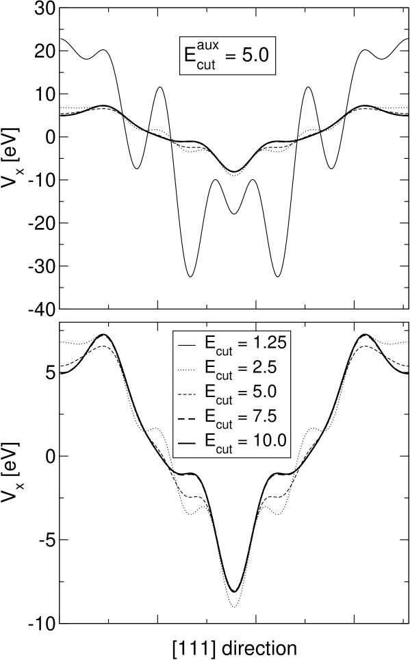
Figure 1: xOEP exchange potential along the silcion-silicon bond axis, i.e., the unit cell’s diagonal, for an auxiliary basis set cutoff $E_{cut}^{aux}=5.0\,a.u.$ and different orbital basis set cutoffs $E_{cut}$. The upper and lower panels differ in the energy scale. The curve for $E_{cut}=1.25\,a.u.$ is only displayed in the upper panel.

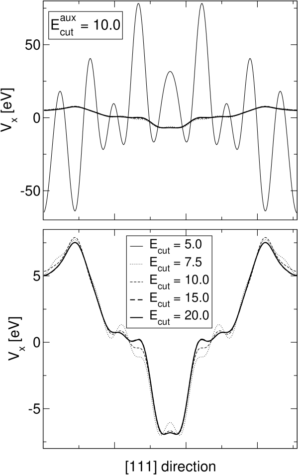
Figure 2: xOEP exchange potential along the silcion-silicon bond axis, i.e., the unit cell’s diagonal, for an auxiliary basis set cutoff $E_{cut}^{aux}=10.0\,a.u.$ and different orbital basis set cutoffs $E_{cut}$. The upper and lower panels differ in the energy scale. The curve for $E_{cut}=5.0\,a.u.$ is only displayed in the upper panel.

Figs. 1 and 2 display xOEP exchange potentials along the silcion-silicon bond axis, i.e., the unit cell’s diagonal, for auxiliary basis set cutoffs $E_{cut}^{aux}$ of 5.0 and 10.0 a.u. ($G_{cut}^{aux}$ of 3.2 and 4.5 a.u.), and for various different orbital basis set cutoffs $E_{cut}$. Note that in figures and tables instead of the cutoffs $G_{cut}$ and $G_{cut}^{aux}$ that refer to the length of the reciprocal lattice vectors of the plane waves the corresponding energy cutoffs $E_{cut}=\frac{1}{2}G_{cut}^{2}$ and $E_{cut}^{aux}=\frac{1}{2}(G_{cut}^{aux})^{2}$ are displayed. Fig. 1 shows that the combination of an auxiliary basis set with cutoff $E_{cut}^{aux}=5.0$ ($G_{cut}^{aux}=3.2$) with a orbital basis set with cutoff $E_{cut}=1.25$ ($G_{cut}=1.6$) leads to a highly oscillating unphysical exchange potential. The cutoff of the auxiliary basis set in the considered case is about twice as large as the cutoff of the orbital basis. This means that the space spanned by the auxiliary basis is the same as that of all products of occupied and unoccupied orbitals. In this case the matrix representing the response function is corrupted and the resulting exchange potential turns out to be unphysical. With increasing cutoff $E_{cut}$ of the orbital basis set the xOEP exchange potentials converge towards the physical KS exchange potential, more precisely towards the representation of the physical KS exchange potential in an auxiliary basis set with cutoff $E_{cut}^{aux}=5.0$ ($G_{cut}^{aux}=3.2$). If the cutoff $E_{cut}$ of the orbital basis set is about 1.5 times as large as the cutoff of the auxiliary basis set $E_{cut}^{aux}$, i.e., equals 7.5 ($G_{cut}=3.9$), then the exchange potential is converged. A further increase of $E_{cut}$ to $E_{cut}=10.0$ ($G_{cut}=4.5$) leads to an exchange potential that is indistinguishable from that for $E_{cut}=7.5$ ($G_{cut}=3.9$) on the scale of Fig. 1. Fig. 2 gives an analogous picture for a cutoff of the auxiliary basis set of $E_{cut}^{aux}=10.0$ ($G_{cut}^{aux}=4.5$). Again, if the space spanned by the auxiliary basis set equals that of the product of occupied and unoccupied orbitals, curve for $E_{cut}=5.0$ ($G_{cut}=3.2$), an highly oscillating unphysical exchange potential is obtained. If $E_{cut}\approx 1.5E_{cut}^{aux}$ then the exchange potential is converged towards the representation of the physical KS exchange potential in an auxiliary basis set with cutoff $E_{cut}^{aux}=10.0$ ($G_{cut}^{aux}=4.5$).

This demonstrates the point that the xOEP scheme only represents a KS scheme if the orbital basis set is balanced to the auxiliary basis set. In the case of a plane wave basis set this requires the energy cutoff $E_{cut}$ of the orbital basis set to be about 1.5 times larger than the energy cutoff $E_{cut}^{aux}$ of the auxiliary basis set.

Table 1 lists for a number of orbitals basis set cutoffs $E_{cut}$ exchange and ground state energies for series of auxiliary basis set cutoffs $E_{cut}^{aux}$. Table 1 shows that the ground state energies for a given $E_{cut}$ always decrease with increasing $E_{cut}^{aux}$ even if the values of $E_{cut}^{aux}$ is that large that the resulting exchange potential is unphysical. This demonstrates that the xOEP scheme remains well-defined even if unbalanced basis sets are used. In this case, however, the xOEP scheme no longer represents a KS method and the resulting exchange potential is unphysical and does not represent the KS exchange potential. Table 1 also lists the differences of the xOEP and HF ground state energies and shows that the xOEP energy does not converge to the HF energy. In the combinations $E_{cut}=2.5/E_{cut}^{aux}=10.0$, $E_{cut}=5.0/E_{cut}^{aux}=20.0$, and $E_{cut}=7.5/E_{cut}^{aux}=29.9$ the space spanned by the auxiliary basis set roughly equals that of the product of occupied and unoccupied orbitals. The ground state xOEP energies in these cases is de facto the lowest that can be achieved by the xOEP method for the given orbital basis set. The fact that this energy is higher than the HF total energy shows that the xOEP energy does not reach the HF ground state energy if the products of occupied and unoccupied orbitals become linearly dependent as it is usually the case in plane wave calculations and as it is the case in the presented calculations.

V Summary

We have given arguments leading to the conclusion that exchange-only optimized potential (xOEP) methods, with finite basis sets, cannot in general yield the Hartree-Fock (HF) ground state energy, but a ground state energy that is higher. This holds true even if the exchange potential that is optimized in xOEP schemes is expanded in an arbitrarily large auxiliary basis set. The HF ground state energy can only be obtained via an xOEP scheme in the special case that all products of occupied and unoccupied orbitals emerging for the orbital basis set are linearly independent from each other. In this case, however, exchange potentials leading to the HF ground state energy exhibit unphysical oscillations and do not represent Kohn-Sham (KS) exchange potentials. These findings solve the seemingly paradoxical results of Staroverov, Scuseria and Davidson staroverov06 that certain finite basis set xOEP calculations lead to the HF ground state energy despite the fact that it was shown ivanov03 that within a real space representation (complete basis set) the xOEP ground state energy is always higher than the HF energy. A key point is that the orbital products of a complete basis are linearly dependent.

Moreover, whether or not the products of occupied and unoccupied orbitals are linearly independent, we have shown that basis set xOEP methods only represent exchange-only (EXX) KS methods, i.e., proper density-functional methods, if the orbital basis set and the auxiliary basis set representing the exchange potential are balanced to each other, i.e., if the orbital basis set is comprehensive enough for a given auxiliary basis set. Otherwise xOEP schemes do not represent EXX KS methods. We have found that auxiliary basis sets that consist of all products of occupied and unoccupied orbitals are not balanced to the corresponding orbital basis set. The xOEP method, even in cases of unbalanced orbital and auxiliary basis sets, works properly in the sense that it determines among all exchange potentials that can be represented by the auxiliary basis set the one that yields the lowest ground state energy. However, in these cases the resulting exchange potential is unphysical and does not represent a KS exchange potential. Therefore the xOEP method is of little practical use in those cases for which it does not represent a EXX KS method. Remember that, at present, the main reason to carry out xOEP methods in most cases is to obtain a qualitatively correct KS one-particle spectrum, either for the purposes of interpretation or as input for other approaches like time-dependent density-functional methods. However, the unphysical oscillations of the exchange-potential of xOEP schemes with unbalanced basis sets affect the unoccupied orbitals and eigenvalues. Another reason to carry out xOEP methods that represent EXX KS methods is that the latter may be combined with new, possibly orbital-dependent, correlation functionals to arrive at a new generation of density-functional methods. Also in this case it is important that the xOEP methods represents proper KS methods.

A balancing of auxiliary and orbital basis sets is straightforward for plane wave basis sets. In this case xOEP schemes are proper EXX KS methods if the energy cutoff for the orbital basis set set is about 1.5 times as large as that of the auxiliary basis set. This as well as other results of this work were illustrated with plane wave calculations for bulk silicon. For Gaussian basis sets on the other hand, a proper generally applicable and reasonably simple balancing scheme of orbital and auxiliary basis sets is so far not available despite much efforts gorling99 ; ivanov99 ; hamel01 ; veseth01 ; hirata01 ; yang02 . Therefore effective exact exchange-only methods like the KLI krieger92 , the ’localized Hartree-Fock’ dellasala01 , the equivalent ’common energy denominator approximation’ method gritsenko01 , or the closely related very recent method of Ref. staroverov06b, , are in use as numerically stable alternatives that yield results very cose to those of full EXX KS methods.

Table 1: xOEP exchange and ground state energies $E_{\mathrm{x}}^{\mathrm{xOEP}}$ and $E^{\mathrm{xOEP}}$, respectively, and the difference between HF and xOEP ground state energy for various combinations of and orbital auxiliary basis sets, characterized by energy cutoffs $E_{cut}$ and $E_{cut}^{aux}$, respectively. ($N$ and $M^{\mathrm{aux}}$ denote the corresponding number of basis functions.) All quantities are given in a.u.

$E_{cut}$ / $N$	$E_{cut}^{aux}$	$M^{\mathrm{aux}}$	$E_{x}^{xOEP}$	$E^{xOEP}$	$E^{HF}$-ExOEP
2.5 / 59	2.5	59	-2.1423	-7.4028	0.0054
	5.0	137	-2.1434	-7.4033	0.0050
	6.0	181	-2.1463	-7.4043	0.0039
	7.4	259	-2.1474	-7.4051	0.0031
	10.0	411	-2.1479	-7.4053	0.0030
5.0 / 150	2.5	59	-2.1451	-7.5061	0.0077
	5.0	137	-2.1460	-7.5065	0.0073
	7.4	259	-2.1468	-7.5069	0.0070
	10.0	411	-2.1481	-7.5076	0.0062
	14.9	725	-2.1501	-7.5087	0.0051
	20.0	1139	-2.1502	-7.5088	0.0050
7.5 / 274	2.5	59	-2.1482	-7.5269	0.0080
	5.0	137	-2.1487	-7.5272	0.0078
	7.4	259	-2.1494	-7.5274	0.0075
	10.0	411	-2.1495	-7.5275	0.0075
	14.9	725	-2.1520	-7.5286	0.0063
	24.9	1639	-2.1539	-7.5296	0.0053
	29.9	2085	-2.1540	-7.5297	0.0053
10.0 / 415	2.5	59	-2.1489	-7.5287	0.0081
	5.0	137	-2.1494	-7.5290	0.0078
	7.4	259	-2.1500	-7.5292	0.0076
	10.0	411	-2.1501	-7.5292	0.0076
	14.9	725	-2.1505	-7.5294	0.0074
	20.0	1139	-2.1511	-7.5296	0.0072

VI Appendix: Linear dependence of products of basis functions of a complete basis

Let $\{\phi_{k}(x)\}$ be a complete set of functions of a complex valued variable $x$ such that any arbitrary square integrable function can be written as a linear combination of the functions in the complete set. We show that the set $\{\phi_{k}(x)\phi_{l}(x)\}$ is linearly dependent.

Using our complete sets, an arbitrary function $f(x,y)$ of two complex valued variables $x$ and $y$ may be expanded in terms of $\{\phi_{k}(x)\}$ and $\{\phi_{\ell}(y)\}$

$$f(x,y)=\sum_{k=1}^{\infty}\sum_{\ell=1}^{\infty}b_{k,\ell}\,\phi_{\ell}(y)\phi_{k}(x)$$ (30)

Set $y=x$ to get:

$$f(x,x)=\sum_{k=1}^{\infty}\sum_{\ell=1}^{\infty}\,b_{k,\ell}\,\phi_{\ell}(x)\phi_{k}(x)$$ (31)

Now choose a function $f(x,x)$ and a $\phi_{n}(x)$ out of the set $\{\phi_{k}(x)\}$ such that (i) $\lim_{x\to\infty}\frac{f(x,x)}{\phi_{n}(x)}=0$ and (ii) at least one $b_{k,\ell}\neq 0$ when $\ell\neq n$ and $k\neq n$. Since $\frac{f(x,x)}{\phi_{n}(x)}$ is just a function of $x$, we may expand it in term of the $\{\phi_{k}(x)\}$:

$$\frac{f(x,x)}{\phi_{n}(x)}=\sum_{m=1}^{\infty}d_{m}\phi_{m}(x)$$ (32)

Solving for $f(x,x)$,

$$f(x,x)=\phi_{n}(x)\sum_{m=1}^{\infty}d_{m}\phi_{m}(x)=\sum_{m=1}^{\infty}d_{m}\phi_{m}(x)\phi_{n}(x)$$ (33)

and equating Eq. (31) with Eq. (33), we get

$$\sum_{m=1}^{\infty}d_{m}\phi_{m}(x)\phi_{n}(x)=\sum_{k=1}^{\infty}\sum_{\ell=1}^{\infty}b_{k,\ell}\phi_{k}(x)\phi_{\ell}(x)$$ (34)

or by setting $k=m$,

$$\sum_{m=1}^{\infty}d_{m}\phi_{m}(x)\phi_{n}(x)-\sum_{m=1}^{\infty}\sum_{\ell=1}^{\infty}b_{m,\ell}\phi_{m}(x)\phi_{\ell}(x)=0$$ (35)

or

$$(d_{n}-b_{n,n})\phi_{n}(x)\phi_{n}(x)+\sum_{\begin{subarray}{c}j=1\\ j\neq n\end{subarray}}^{\infty}(d_{j}-b_{j,n}-b_{n,j})\phi_{n}(x)\phi_{j}(x)-\sum_{\begin{subarray}{c}\ell=1\\ \ell\neq n\end{subarray}}^{\infty}\sum_{\begin{subarray}{c}m=1\\ m\neq n\end{subarray}}^{\infty}b_{m,\ell}\phi_{m}(x)\phi_{\ell}(x)=0\,.$$ (36)

Eq. (36) is a linear combination of a subset of $\{\phi_{k}(x)\phi_{l}(x)\}$ broken up into disjoint components and equated to zero. If a subset of a set is linearly dependent, then the set must also be linearly dependent. We show such a case by contradiction: According to Eq. (36), for the subset $\{\phi_{k}(x)\phi_{l}(x)\}_{\subset}$ (appearing in the equation) to be linearly independent, three conditions must be met:

1. $d_{n}=b_{n,n}$

2. $d_{j}-b_{j,n}-b_{n,j}=0$ ($\forall$ $j\in\mathbb{N}$ with $j\neq n$)

3. $b_{m,\ell}=0$ ($\forall$ $m,\ell\in\mathbb{N}$ with $m\neq n$ and $\ell\neq n$)

But according to our condition on $f(x,x)$ there is at least one $b_{m,\ell}\neq 0$ with $m\neq n$ and $\ell\neq n$, which is a contradiction to number three of our linear independence criteria. Therefore $\{\phi_{k}(x)\phi_{l}(x)\}_{\subset}$ must be linearly dependent by contradiction, and therefore $\{\phi_{k}(x)\phi_{l}(x)\}$ for all $k,l\in\mathbb{N}$ is linearly dependent because $\{\phi_{k}(x)\phi_{l}(x)\}_{\subset}$ is linearly dependent.

One may take the result one step further to show with an induction argument that for any complete set such as $\{\phi_{k}(x)\}$ the set defined by $\{\prod_{i=1}^{N}\phi_{p_{i}}(x)|$ $N,i,p_{i}\in\mathbb{N}$} is complete and linearly dependent.

References

- (1) V. K. Staroverov, G. E. Scuseria, and E. R. Davidson, J. Chem. Phys. 124, 141103 (2006).
- (2) V. Sahni, J. Gruenbaum, and J. P. Perdew, Phys. Rev. B 26, 4371 (1982).
- (3) S. Ivanov and M. Levy, J. Chem. Phys. 119, 7087 (2003).
- (4) M. Städele, J. A. Majewski, P. Vogl, and A. Görling, Phys. Rev. Lett. 79, 2089 (1997).
- (5) M. Städele, M. Moukara, J. A. Majewski, P. Vogl, and A. Görling, Phys. Rev. B 59, 10031 (1999).
- (6) R. J. Magyar, A. Fleszar, and E.K.U. Gross, Phys. Rev. B 69, 045111 (2004).
- (7) A. Qteish, A.I. Al-Sharif, M. Fuchs, M. Scheffler, S. Boeck, and J. Neugebauer, Comp. Phys. Comm. 169, 28 (2005).
- (8) P. Rinke, A. Qteish, J. Neugebauer, C. Freysoldt, and M. Scheffler, New J. Phys. 7, 126 (2005).
- (9) A. Görling and M. Ernzerhof, Phys. Rev. A 51, 4501 (1995).
- (10) R. T. Sharp and G. K. Horton, Phys. Rev. 90, 317 (1953).
- (11) J. D. Talman and W. F. Shadwick, Phys. Rev. A 14, 36 (1976).
- (12) W. Kohn and L. J. Sham, Phys. Rev. 140, A1133 (1965).
- (13) M. Levy, Proc. Natl. Acad. Sci. USA 76, 6062 (1979).
- (14) J. E. Harriman, Phys. Rev. A 27, 632 (1983); 34, 29 (1986).
- (15) M. Levy and J. A. Goldstein, Phys. Rev. B 35, 7887 (1987).
- (16) See the ’constrained search‘ discussion in Ref [ivanov03, ], which includes appropriate references on the approach in this context .
- (17) H. Ou-Yang and M. Levy, Phys. Rev. Lett. 65, 1036 (1990).
- (18) M. Levy and J. P. Perdew, Phys. Rev. A32, 2010 (1985).
- (19) M. Levy and A. Görling, Phys. Rev. A 53, 3140 (1996).
- (20) A. Görling and M. Levy, Int. J. Quantum Chem. Symp. 29, 93 (1995).
- (21) A. Görling, J. Chem. Phys. 123, 062203 (2005); and references therein.
- (22) P. Carrier, S. Rohra, and A. Görling, submitted.
- (23) E. Engel, A. Höck, and S. Varga, Phys. Rev. B 63, 125121 (2001).
- (24) E. Engel, A. Höck, R. N. Schmid, and R. M. Dreizler Phys. Rev. B 64, 125111 (2001).
- (25) A. Görling, Phys. Rev. Lett. 83, 5459 (1999).
- (26) S. Ivanov, S. Hirata, and R. J. Bartlett, Phys. Rev. Lett. 83, 5455 (1999).
- (27) S. Hamel, M. E. Casida, and D. R. Salahub, J. Chem. Phys. 114, 7342 (2001).
- (28) L. Veseth, J. Chem. Phys. 114, 8789 (2001).
- (29) S. Hirata, S. Ivanov, I. Grabowski, R. Bartlett, K. Burke, and J. D. Talman, J. Chem. Phys. 115, 1635 (2001).
- (30) W. Yang and Q. Wu, Phys. Rev. Lett. 89, 143002 (2002).
- (31) J. B. Krieger, Y. Li, and G. J. Iafrate, Phys. Rev. A 46, 5453 (1992).
- (32) F. Della Sala and A. Görling, J. Chem. Phys. 115, 5718 (2001).
- (33) O. V. Gritsenko and E. J. Baerends, Phys. Rev. A 64, 042506 (2001).
- (34) V. K. Staroverov, G. E. Scuseria, and E. R. Davidson, J. Chem. Phys. 125, 081104 (2006).