Broken spin-Hall accumulation symmetry by magnetic field
and coexisted Rashba and Dresselhaus interactions

Abstract

The spin-Hall effect in the two-dimensional electron gas (2DEG) generates symmetric out-of-plane spin $S_{z}$ accumulation about the current axis, in the absence of external magnetic field. Here we employ the real space Landauer-Keldysh formalismKel by considering a four-terminal setup to investigate the circumstances in which this symmetry is broken. For absence of Dresselhaus interaction, starting from the applied out-of-plane $B$ corresponding to Zeeman splitting energy $\Delta=0$ to $0.5$ times the Rashba hopping energy $t_{SO}^{R}$, the breaking process is clearly seen. The influence of the Rashba interaction on the magnetization of the 2DEG is studied herein. For coexisted Rashba $t_{SO}^{R}$ and Dresselhaus $t_{SO}^{D}$ spin-orbit couplings in the absence of $B$, interchanging $t_{SO}^{R}$ and $t_{SO}^{D}$ reverses the entire accumulation pattern.

The generation and transport of spin currents dominates the applications of spintronics. The spin-orbit (SO) interaction, which couples the electric degree of freedom with the magnetic one serves as the mechanism to achieve this. A number of basic designs${}^{\text{\cite[cite]{\@@bibref{Authors Phrase1YearPhrase2}{design}{\@@citephrase{(}}{\@@citephrase{)}}}}}$ for spintronic devices, such as field-effect switches, spin transistors, spin filters, and spin waveguides, have been proposed by taking advantage of this interaction to control spins. One of the phenomena originating from the SO interaction is the spin-Hall (SH) effect${}^{\text{\cite[cite]{\@@bibref{Authors Phrase1YearPhrase2}{Sinova}{\@@citephrase{(}}{\@@citephrase{)}}}}}$ in which a transverse spin current is induced by a longitudinal electrical current. The semiclassical SO force${}^{\text{\cite[cite]{\@@bibref{Authors Phrase1YearPhrase2}{SOforce}{\@@citephrase{(}}{\@@citephrase{)}}}}}$ proportional to $(\mathbf{p}\times\mathbf{e}_{z})\sigma$, oppositely deflects the spin up ($\sigma=1$) and down ($\sigma=-1$) wave packets with momentum $\mathbf{p}$ in the transverse directions so that different spins accumulate in the lateral edges. The effect is particularly notable in that it produces a spin current with no magnetic field applied, and no accompanying charge current present. Recent experimental work using scanning Kerr microscopy${}^{\text{\cite[cite]{\@@bibref{Authors Phrase1YearPhrase2}{experiment1,experiment2,experiment3,experiment4}{\@@citephrase{(}}{\@@citephrase{)}}}}}$ in n-type unstrained GaAs, strained InGaAs${}^{\text{\cite[cite]{\@@bibref{Authors Phrase1YearPhrase2}{experiment1}{\@@citephrase{(}}{\@@citephrase{)}}}}}$ and 2DEG,${}^{\text{\cite[cite]{\@@bibref{Authors Phrase1YearPhrase2}{experiment3}{\@@citephrase{(}}{\@@citephrase{)}}}}}$ have inspired a host of theoretical studies on SH effect.

The 2DEG confined in the InGaAs/InAlAs semiconductor heterostructure${}^{\text{\cite[cite]{\@@bibref{Authors Phrase1YearPhrase2}{heture}{\@@citephrase{(}}{\@@citephrase{)}}}}}$ possesses intrinsic SO coupling known as the Rashba and Dresselhaus interactions. The inversion asymmetry of the structure gives this system the Rashba interaction with adjustable strength via the gate voltage${}^{\text{\cite[cite]{\@@bibref{Authors Phrase1YearPhrase2}{heture,Das}{\@@citephrase{(}}{\@@citephrase{)}}}}}$ while the bulk inversion asymmetry${}^{\text{\cite[cite]{\@@bibref{Authors Phrase1YearPhrase2}{Dresselhaus}{\@@citephrase{(}}{\@@citephrase{)}}}}}$ gives rise to the Dresselhaus interaction whose strength is material dependent. A number of studies regarding the intrinsic SH (ISH) effect in the 2DEG have been reported, but most of these focus on evaluating the spin current which is, due to its nonconservation, not easily measured. The SO coupling leads an electron to precess around a momentum-dependent effective magnetic field which produces a source or a sink of the spin current in the continuity equation. Due to this nonconservation the spin current is not uniquely defined.${}^{\text{\cite[cite]{\@@bibref{Authors Phrase1YearPhrase2}{notuni1,notuni2}{\@@citephrase{(}}{\@@citephrase{)}}}}}$ Although a possible definition of a conserved spin current has been suggested in Ref. condef, , the present work follows Ref. Kel, by employing the Landauer-Keldysh formalism in the four-terminal setup to investigate a more directly measurable physical quantity: the accumulation of the out-of-plane spin $S_{z}$. If only the Rashba interaction exists then the accumulation induced by the electric potential deposits spins symmetrically along the transverse direction, i.e., the up-spins accumulate on one side while the down-spins accumulate symmetrically on the other. The majority of current studies focuses on how this SH symmetry (SHS) is generated. By contrast, in the paper we answer the essential question of the circumstances under which the SHS is broken.

With the help of the finite difference method,${}^{\text{\cite[cite]{\@@bibref{Authors Phrase1YearPhrase2}{Dattabook}{\@@citephrase{(}}{\@@citephrase{)}}}}}$ the linear Rashba and Dresselhaus model with applied field $B$ is, in the tight binding limit, expressed as

$$\hat{H}^{\left(c\right)} =\sum_{\mathbf{m\sigma}}\varepsilon_{\mathbf{m}}c_{\mathbf{m\sigma}}^{\dagger}c_{\mathbf{m\sigma}}$$ (1)

$$+\sum_{\mathbf{mm}^{\prime}\sigma\sigma^{\prime}}c_{\mathbf{m}\sigma}^{\dagger}t_{\mathbf{mm}^{\prime}}^{\sigma\sigma^{\prime}}c_{\mathbf{m}^{\prime}\sigma^{\prime}}+\sum_{\mathbf{m\sigma}}\sigma\frac{\Delta}{2}c_{\mathbf{m\sigma}}^{\dagger}c_{\mathbf{m\sigma}},$$

where $c_{\mathbf{m}\sigma}^{\dagger}$ ($c_{\mathbf{m}^{\prime}\sigma^{\prime}}$) denotes the creation (annihilation) operator for $\sigma=+1$ (spin-up) or $\sigma=-1$ (spin-down) at the site $\mathbf{m}=(\mathbf{m}_{x},\mathbf{m}_{y})$. The electric potential and disorder can be accounted for by the on-site energy $\varepsilon_{\mathbf{m}}$. To see how SHS is destroyed either by $B$ or coexisted Dresselhaus and Rashba interactions, we consider the clean limit and set the tight-binding bottom energy, for convenience, to be $-4t_{0}$ (corresponding to $\varepsilon_{\mathbf{m}}=0$), with $t_{0}=\hbar^{2}/2ma^{2}$ being the hopping energy. The Zeeman splitting $\Delta=-e\hbar B/mc$ is induced by the magnetic field while the Rashba (Dresselhaus) SO coupling $t_{SO}^{R(D)}=\alpha(\beta)/2a$ is taken into account by the neareast-neighbor hopping matrix element $t_{\mathbf{mm}^{\prime}}^{\sigma\sigma^{\prime}}=\left\langle\sigma\right|-t_{0}I_{s}-it_{SO}^{R}\sigma_{y}-it_{SO}^{D}\sigma_{x}|\sigma^{{}^{\prime}}\rangle$ for $\mathbf{m}=\mathbf{m}^{\prime}+\mathbf{e}_{x}$, and $\left\langle\sigma\right|-t_{0}I_{s}+it_{SO}^{R}\sigma_{x}+it_{SO}^{D}\sigma_{y}|\sigma^{{}^{\prime}}\rangle$ for $\mathbf{m}=\mathbf{m}^{\prime}+\mathbf{e}_{y}$. Here the identity matrix in spin space is $I_{s}$, the lattice constant is $a$, and the Rashba (Dresselhaus) coupling strength is $\alpha$ ($\beta$). In order to subject the conductor to an electric potential difference along the $x$ axis we consider the Landauer setup with the four ideal leads $p=1$ (left), $2$ (right), $3$ (bottom)$,4$ (top) shown in Fig. 1(a).

To acquaint the reader with the method employed herein we present here a brief review of the Landauer-Keldysh Formalism. In general, in a conductor the non-equilibrium spin accumulation at time $t$, $\left\langle S_{\mathbf{m}}^{z}(t)\right\rangle$ $=\hbar/2\sum_{\sigma}\sigma\left\langle c_{\mathbf{m\sigma}}^{\dagger}(t)c_{\mathbf{m\sigma}}(t)\right\rangle=\hbar/2\sum_{\sigma}\sigma\left[\left\langle\mathbf{m}\sigma\right|\mathbf{G}^{<(c)}(t,t)\left|\mathbf{m}\sigma\right\rangle\hbar/i\right],$ depends on the switching time $t_{s}$ (at which leads are brought into contact) via the lesser Green function

$$\mathbf{G}^{<\left(c\right)}(t_{1},t_{1}^{{}^{\prime}})$$ (2)

$$=\int_{t_{s}}^{\infty}dt_{2}\int_{t_{s}}^{\infty}dt_{3}\mathbf{G}^{r\left(c\right)}(t_{1},t_{2})\mathbf{\Sigma}^{<\left(c\right)}(t_{2,}t_{3})\mathbf{G}^{r\left(c\right)\dagger}(t_{3},t_{1}^{{}^{\prime}})$$

$$+\mathbf{G}^{r\left(c\right)}(t_{1},t_{s})\mathbf{G}^{<\left(c\right)}(t_{s},t_{s})\mathbf{G}^{r\left(c\right){\dagger}}(t_{s},t_{1}^{\prime}),$$

which includes both the steady state (second line), and also the transient state (third line). For the measuring time $t$ much later than $t_{s}$ (this is the case of interest here) one can approximately write in Eq. (2) $t_{s}=-\infty$. The transient solution can then be neglected, and $\mathbf{G}^{<(c)}(t_{1},t_{1}^{{}^{\prime}})$ $=\mathbf{G}^{<(c)}(\tau)$ depends only on the the time interval $\tau\equiv t_{1}-t_{1}^{\prime}.$ A Fourier transformation of Eq. (2) then yields the kinetic equation

$$\mathbf{G}^{<(c)}(E)=\mathbf{G}^{r(c)}(E)\mathbf{\Sigma}^{<(c)}(E)\mathbf{G}^{r(c)\dagger}(E)$$ (3)

with the retarded Green function $\mathbf{G}^{r(c)}(E)=[E-\mathbf{H}^{(c)}-\mathbf{\Sigma}^{(c)}(E)]^{-1}$, so that the steady accumulation is expressed as $S_{\mathbf{m}}^{z}(t=0)=\frac{\hbar}{2}\sum_{\sigma\sigma^{\prime}=\pm 1}\left\langle\sigma\right|\mathbf{\sigma}_{z}|\sigma^{{}^{\prime}}\rangle\int_{-\infty}^{\infty}dE(\mathbf{G}(E)^{<(c)})_{\mathbf{mm}\sigma^{\prime}\sigma}/2\pi i$. The lead interacts with the conductor through the self-energy${}^{\text{\cite[cite]{\@@bibref{Authors Phrase1YearPhrase2}{Dattabook}{\@@citephrase{(}}{\@@citephrase{)}}}}}$ $\mathbf{\Sigma}^{(c)}=\sum_{p}\mathbf{\Sigma}_{p}^{(c)},$ with matrix elements $\left\langle\mathbf{m,}\sigma\right|\mathbf{\Sigma}_{p}^{(c)}|\mathbf{m}^{\prime},\sigma^{{}^{\prime}}\rangle\equiv\Sigma_{p\mathbf{m},\mathbf{m}^{\prime}}^{(c)\sigma\sigma^{\prime}}=t_{0}^{2}g^{(p)}(\mathbf{r}_{\mathbf{m}},\mathbf{r}_{\mathbf{m}^{\prime}}^{\prime})\delta_{\sigma\sigma^{\prime}}$ for $\mathbf{m}$ and $\mathbf{m}^{\prime}$ (in the conductor) being adjacent points to $\mathbf{r}_{\mathbf{m}}$ and $\mathbf{r}_{\mathbf{m}^{\prime}}^{\prime}$ (in leads), and $\Sigma_{p\mathbf{m},\mathbf{m}^{\prime}}^{(c)\sigma\sigma^{\prime}}=0$ otherwise. The hopping energy $t_{0}$ for these points allows electrons to flow through the interfaces. While the lesser self-energy is written as

$$\mathbf{\Sigma}^{<(c)}(E)=-2i\operatorname{Im}\mathbf{\Sigma}_{p}(E-eV_{p})f(E-eV_{p}),$$ (4)

where $f(E)=1/\left[1+\exp(-E/k_{B}T)\right]$ is the Fermi-Dirac distribution and the quasi-particle escaping time, in the conductor, is inversely proportional to $\operatorname{Im}\mathbf{\Sigma}^{(c)}(E)$. The retarded Green function $\hat{g}^{(p)}$ for the isolated lead $p$ can be evaluated by considering the single particle Green operator $\hat{g}^{(p)}=1/(E+i0_{+}-\hat{H}^{(p)})$ in the eigenfunction expansion $g^{(p)}(\mathbf{r}_{1},\mathbf{r}_{2})=\sum_{n\gamma}\psi_{n\gamma}^{(p)}(r_{1l},r_{1t})\psi_{n\gamma}^{(p)\ast}(r_{2l},r_{2t})/(E+i0_{+}-\varepsilon_{n\gamma}^{(p)})$, where $\mathbf{r=(}r_{l},$ $r_{t})$ is the position vector (within the lead) composed by the longitudinal component $r_{l}$ and the transverse component $r_{t}$ with $n$ and $\gamma$ accounting the transverse and longitudinal modes, respectively. The eigenfunction $\psi_{n\gamma}^{\left(p\right)}\left(r_{l},r_{t}\right)=2\sin(n\pi r_{t}/W)\sin(\gamma\pi r_{l}/L)/(a\sqrt{WL})$, with the normalization $\sum_{n\gamma}$ $\psi_{n\gamma}^{(p)}(\mathbf{r}^{\prime})\psi_{n\gamma}^{(p)\ast}(\mathbf{r)}=\delta_{\mathbf{rr}^{\prime}}$, is obtained by solving the eigenequation $\hat{H}_{p}\psi_{n\gamma}^{(p)}(r_{l},r_{t})=[-(\hbar^{2}/2m)d^{2}/dr_{l}^{2}+V_{conf}^{(p)}(r_{t})]\psi_{n\gamma}^{(p)}(r_{l},r_{t})=\varepsilon_{n\gamma}\psi_{n\gamma}^{(p)}(r_{l},r_{t})$ under the hard-wall boundary condition in which the confining potential $V_{conf}^{(p)}$ $=$ $\infty$ ($0$) outside (inside) the lead $p$. The width (length) of the lead is $W$ ($L$). For semi-infinite lead $L\rightarrow\infty$, $g^{(p)}(\mathbf{r}_{1},\mathbf{r}_{2})$ can be directly computed by replacing the summation of longitudinal modes $\sum_{\gamma}$ with $\int_{0}^{\infty}d\gamma L/\pi.$

Consider now the InGaAs/InAlAs heterostructure${}^{\text{\cite[cite]{\@@bibref{Authors Phrase1YearPhrase2}{heture}{\@@citephrase{(}}{\@@citephrase{)}}}}}$ with typical parameters. The effective mass $m=0.05m_{e}$ ($m_{e}$ is the electron mass) and the lattice constant $a=3$ nm yield the hopping energy $t_{0}=84.68$ m$\operatorname{eV}$. We set $t_{SO}^{R}=0.1t_{0}$, $eV_{1}=-eV_{2}=eV/2$, $eV_{3}=eV_{4}=0$, $eV=10^{-3}t_{0}$ and conductor size to be $8a\times 8a$. Select the Fermi energy $E_{F}=-3.8t$ close to the band bottom at $-4t_{0},$ so that the tight-binding approximation valid. To examine how $\Delta$ and the coexistence of $t_{SO}^{R}$ and $t_{SO}^{D}$ affect the SHS, we show the spatial $S_{z}$ accumulation in units of $\hbar/2$ in Fig. 1 (with $t_{SO}^{D}=0$) and Fig. 2 (with $\Delta=0$).

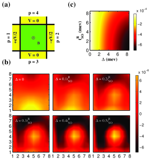
Figure 1: (Color online) (a) Illustration of the Landauer four-terminal setup with the out-of-plane $B$. Contacting the 2DEG (green square) with four ideal semi-infinite leads (yellow rectangles) $p=1$ (left), $2$ (right), $3$ (bottom), $4$ (top) which are biased with $eV_{1}=-eV_{2}=eV/2$, $eV_{3}=eV_{4}=0$ and $eV=10^{-3}t_{0},$ the spatial out-of-plane $S_{z}$ accumulations, in units of $\hbar/2$ with Zeeman splitting $\Delta$ being varied from $0$ to $0.5t_{SO}^{R}$, are plotted in (b). The magnetization, obtained by summing over every accumulation on each site, in units of $\hbar/2$, decreases with $t_{SO}^{R}$ but increases with $\Delta$ as shown in (c).

Obviously, the applied field $B$ polarizes the 2DEG or, from perspective of the band theory, it induces a Zeeman splitting $\Delta$ such that the SHS is destroyed. Starting from $\Delta=0$ and going to $\Delta=0.5t_{SO}^{R},$ two effects are found to break the symmetry [see Fig. 1(b)]: (i) The area of the majority spins is enlarged. (ii) The magnitude of the majority magnetization is increased. On the other hand, for parameters $\Delta$ and $t_{SO}^{R}$ varying between $0$ and $0.1t_{0}$, the magnetization (or the total $z$-polarization) of the system, obtained by summing over every $S_{z}$ on each site, is decreased with increasing Rashba interaction as shown in [Fig. 1(c)]. To explain this, we note that, under the Rashba interaction, electrons precess with respect to an in-plane ($x$-$y$) effective Rashba magnetic field which yields vanishing mean $z$-polarization so that magnetization is reduced.

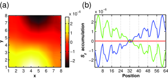
Figure 2: (Color online) (a) The spatial $S_{z}$ accumulation with $\left(t_{SO}^{R},t_{SO}^{D}\right)=\left(0.1t_{0},0.05t_{0}\right).$ (b) The $S_{z}$ accumulations in units of $\hbar/2$ as functions of positions with parameters $\left(t_{SO}^{R},t_{SO}^{D}\right)=\left(0.1t_{0},0.05t_{0}\right)$ (green) and $\left(t_{SO}^{R},t_{SO}^{D}\right)=\left(0.05t_{0},0.1t_{0}\right)$ (blue). The red line sums up these two functions.

Even $B$ is absent, the SHS can also be broken by the coexistence of $t_{SO}^{R}$ and $t_{SO}^{D}$. Consider the Dresselhaus coupling $t_{SO}^{D}=0.1t_{0}$ ($0.05t_{0}$), corresponding to $\beta\thickapprox\gamma\left\langle k_{z}^{2}\right\rangle=0.5$ ($0.025$) $\operatorname{eV}\operatorname{\text{\AA}}$, assuming a $z$ direction quantum well width $22$ $\operatorname{\text{\AA}}$ ($31\operatorname{\text{\AA}}$) with typical value of the coefficient${}^{\text{\cite[cite]{\@@bibref{Authors Phrase1YearPhrase2}{Knap}{\@@citephrase{(}}{\@@citephrase{)}}}}}$ $\gamma=25$ $\operatorname{eV}\operatorname{\text{\AA}}^{3}$. Our results indicate that the SHS is preserved by the presence of $t_{SO}^{R}$ or $t_{SO}^{D}$ alone, but it is destroyed if the Rashba and Dresselhaus interactions coexist. Figure 2(a) shows the accumulation pattern for $t_{SO}^{R}=0.1t_{0}$, $t_{SO}^{D}=0.05t_{0}$, and $B=0$. In comparison to the $\Delta=0$ result of Fig. 1(b) it is tilted upwards in the left hand region, and downwards in the right hand region. Furthermore, if the strength of the Rashba $t_{SO}^{R}$ and the Dresselhaus $t_{SO}^{D}$ interactions is interchanged then the pattern is entirely reversed, i.e., the up (down) accumulation becomes the down (up) accumulation. To illustrate this effect we label the spin component $S_{z}$ by numbering the position of each site row by row. For example, $\mathbf{m}=(a,a)$ is labeled by position $1$ and $\mathbf{m}=(8a,8a)$ is labeled by position $64$. The accumulation of the component $S_{z}$ in the absence of the field $B$ is plotted in Fig. 2(b) as a function of position for two special cases: (i) $\left(t_{SO}^{R},t_{SO}^{D}\right)=\left(0.1t_{0},0.05t_{0}\right)$ denoted by the green line, and (ii) $\left(t_{SO}^{R},t_{SO}^{D}\right)=\left(0.05t_{0},0.1t_{0}\right)$ denoted by the blue line. Summing up these two functions at every position we obtain zero accumulation everywhere (the red line). This suggests an inverse correlation between the cases (i) and (ii). In the case of equal strengths, $t_{SO}^{R}=t_{SO}^{D}$, one therefore expects that $S_{z}$ accumulates nowhere, since swapping $t_{SO}^{R}$ and $t_{SO}^{D}$ has no effect. Finally, we recall that we address a finite 2DEG. Comparing our results with previous works on infinite systems we identify the predicted sign change${}^{\text{\cite[cite]{\@@bibref{Authors Phrase1YearPhrase2}{Sign}{\@@citephrase{(}}{\@@citephrase{)}}}}}$ in the spin-Hall conductivity.

In conclusion, we investigate the out-of-plane $S_{z}$ spin accumulation using the Landauer-Keldysh formalism in a four terminal setup. Taking into account the Rashba $t_{SO}^{R}$ and the Dresselhaus $t_{SO}^{D}$ couplings and Zeeman splitting $\Delta$ we obtain an accumulation pattern different from the one which results from pure Rashba interactions. In particular, destructions of the SHS are found in two special cases: in the presence of a magnetic field $B$ and in the presence of coexisting Rashba and Dresselhaus couplings. In the former case, beginning with both $\Delta=0$ and $t_{SO}^{D}=0$, the applied field $B$ breaks the SHS by not only extending the area of the majority spin accumulation, but also by strengthening its magnitude. Meanwhile, the gate-voltage-tunable Rashba interaction reduces the magnetization induced by the Zeeman splitting. In the latter case (where both SO couplings are present), interchanging the Rashba and Dresselhaus interactions reverses the whole accumulation pattern. These features thus provide an electric control of a magnetic property.

This work is supported by the Republic of China National Science Council Grant No. 95-2112-M-002-044-MY3.

References

• (1) B. K. Nikolić, S. Souma, L. P. Zârbo, and J. Sinova, Phys. Rev. Lett. 95, 046601 (2005); B. K. Nikolić, L. P. Zârbo, and S. Souma, Phys. Rev. B 73, 075303 (2006).
• (2) S. Datta and B. Das, Appl. Phys. Lett. 56, 665 (1990); J. Nitta et al., Appl. Phys. Lett. 75, 695 (1999); Francisco Mireles and George Kirczenow, Phys. Rev. B 64, 024426 (2001); T. Koga et al., Phys. Rev. Lett. 88, 126601 (2002); X. F. Wang et al., Phys. Rev. B 65, 165217 (2002); D. Frustaglia and K. Richter, Phys. Rev. B 69, 235310 (2004); J. Carlos Egues, Guido Burkard, D. S. Saraga, John Schliemann, and Daniel Loss, Phys. Rev. B 72, 235326 (2005).
• (3) J. Sinova, D. Culcer, Q. Niu, N.A. Sinitsyn, T. Jungwirth, and A.H. MacDonald, Phys. Rev. Lett. 92, 126603 (2004).
• (4) Branislav K. Nikolić, Liviu P. Zârbo, and Sven Welack, Phys. Rev. B 72, 075335 (2005).
• (5) Y.K. Kato, R.C. Myers, A.C. Gossard, D.D. Awschalom, Science 306 1910 (2004).
• (6) J. Wunderlich, B. Kaestner, J. Sinova, and T. Jungwirth, Phys. Rev. Lett. 94, 047204 (2005).
• (7) V. Sih, R.C. Myers, Y.K. Kato, W.H. Lau, A.C. Gossard, D.D. Awschalom, Nature Phys. 1 31 (2005).
• (8) N. P. Stern, S. Ghosh,1 G. Xiang, M. Zhu, N. Samarth, and D. D. Awschalom, Phys. Rev. Lett. 97, 126603 (2006).
• (9) J. Nitta, T. Akazaki, H. Takayanagi, and T. Enoki, Phys. Rev. Lett. 78, 1335 (1997).
• (10) B. Das, D.C. Miller, S. Datta, R. Reifenberger, W.P. Hong, P.K. Bhattacharya, J. Singh, and M. Jaffe, Phys. Rev. B 39, R1411 (1989).
• (11) G. Dresselhaus, Phys. Rev. 100, 580 (1955).
• (12) P. Zhang, J. Shi, D. Xiao, and Q. Niu, cond-mat/0503505.
• (13) S. Murakami, N. Nagaosa and S. C. Zhang, cond-mat/0310005, to appear in Phys. Rev. B.
• (14) J. Shi, P. Zhang, D. Xiao, and Q. Niu, Phys. Rev. Lett. 96, 076604 (2006).
• (15) Supriyo Datta, Electronic Transport in Mesoscopic Systems (Cambridge University Press, 1997).
• (16) W. Knap, C. Skierbiszewski, A. Zduniak, E. Litwin-Staszewska, D. Bertho, F. Kobbi, and J. L. Robert, Phys. Rev. B 53, 3912 (1996).
• (17) N. A. Sinitsyn, E. M. Hankiewicz, W. Teizer, and J. Sinova, Phys. Rev. B 70, 081312(R) (2004).