The non-equilibrium work relation. Thermodynamic analysis and microscopic foundations

Abstract

We discuss the conditions for which the non-equilibrium work relation is valid by means of thermodynamic and microscopic arguments.

1 Introduction

The question of dissipation and the approach to equilibrium in mesoscopic and macroscopic systems has been a long standing problem since the early years of statistical mechanics as a science. Already at the beginning of the XX century Einstein and Ehrenfest were unsatisfied with the fundamental principles of statistical mechanics postulated by Bolztmann and Gibbs, since in their opinion those principles lack of a sound microdynamical basis.PAIS ; COHEN1 ; COHEN2 Their main idea was that the real problem concerns the approach towards the equilibrium state, and not equilibrium in itself. So, the knowledge of the dynamics of the irreversibility and the approach to equilibrium that follows enables one to draw the framework embodying equilibrium as a limiting behavior.

This subject has acquired a renewed interest, mainly due to the technological advances in biophysics and microrheology that make a more detailed analysis of the question possible.liphart ; mackintosh

Related to this problem, attempts have been made to go beyond equilibrium in order to establish some rules for extracting information from irreversible processes. SENGERS ; Groot ; REVIEWjpcb ; pnas ; COHEN-GALLAVOTI ; Jarzynski Recently it has been claimed that there are only a few known relations in statistical mechanics that are valid for systems arbitrarily driven far from equilibrium. One of these relations is the one proposed by Jarzynski Crooks ; Jarzynski for which equilibrium properties can be obtained from non-equilibrium work measurements. For Hamiltonian isolated systems and systems in contact with a heat bath through weak interactions, theoretical justification for this assertion has been given in terms of ensembles of trajectories represented by means of a phase space density.Jarzynski However, from the thermodynamic point of view this assertion seems to be true only for very specific situations.COHEN3 As a consequence, it is important to stipulate the conditions in which one can make use of this relation. On the other hand, the knowledge of the range of applicability of this and other non-equilibrium relations is deeply rooted in the understanding of the microscopic bases of irreversibility.SENGERS ; Groot ; REVIEWjpcb ; pnas ; COHEN-GALLAVOTI

In this article, we will use thermodynamic and statistical arguments to show that the non-equilibrium work relation is valid only in isothermal and near-equilibrium conditions. Moreover, we will revise the validity of the original derivation of this non-equilibrium work relation Jarzynski and then establish a quantitative criterion for determining these conditions by making use of a microscopic theory involving the BBGKY (Bogoliubov-Born-Green-Kirkwood-Yvon) hierarchy of equations balescu .

The paper is organized as follows. In Section 2, we analyze the non-equilibrium work relation by considering the thermodynamic definition of the minimum work done on a system to change its state. After this, in Sec. 3 we analyze the problem of irreversibility in the context of a microscopic theory and propose the entropic time as a quantitative criterion to distinguish quasistatic and nonquasistatic processes. Finally, the last section is devoted to summarize and discuss our main results.

2 Thermodynamics and cumulants

In the very general case, a system driven out of equilibrium does not satisfy the condition of thermal equilibrium with the bath, since the temperature $T$ of the system differs from that of the bath $T_{0}$ ZWANZIG-LIBRO . Among others, typical systems illustrating this situation are glasses and supercooled colloidal fluids.stillinger ; weeks

Since irreversible processes are present in this general case, the total work $R$ performed on the system in order to change its state satisfies the relation LANDAU

$$R\geq\Delta E-T_{0}\Delta S,$$ (1)

where $\Delta E$ and $\Delta S$ are the energy and the entropy variation of the system in the process. Hence, in the case of a reversible process, from Eq. (1) one can infer that the minimum amount of work $R_{min}$ necessary to reverse the state of the system is given by

$$R_{min}=\Delta E-T_{0}\Delta S.$$ (2)

In the isothermal case, when the system is in contact with a heat bath, $T=T_{0}$, Eq. (2) can be used to define the variation of the Helmholtz free energy of the system $\Delta F$

$$R_{min}=\Delta(E-T_{0}S)=\Delta F.$$ (3)

Therefore, thermodynamics requires that the change of the free energy of the system be equal to the work performed on it only in a reversible process in which at least the initial and final states satisfy the thermal equilibrium condition $T=T_{0}$.

In Ref. Jarzynski , the following equation has been established

$$\Delta F=-k_{B}T_{0}\ln\langle e^{-R/k_{B}T_{0}}\rangle,$$ (4)

where $k_{B}$ is the Boltzmann constant and $\langle\,\rangle$ represents the average over an ensemble of measurements of the work $R$.

In view of the thermodynamic relations (1)-(3), one may legitimately ask about the conditions of validity of Eq. (4). To answer this question, it is very important to take into account that, in general, an arbitrary external perturbation will produce an internal irreversible process in which the system approaches equilibrium, in accordance with the Le Chatelier principle.LANDAU

For simplicity we will assume that work is done in isothermal conditions; therefore, we have

$$R=\Delta F+R_{diss},$$ (5)

where $R_{diss}$ is the dissipated work.LANDAU Now, by taking the exponential of Eq. (5) one simply obtains

$$e^{R/k_{B}T_{0}}=e^{\Delta F/k_{B}T_{0}}e^{R_{diss}/k_{B}T_{0}}.$$ (6)

After averaging this expression over the ensemble of measurements of $R$ one obtains

$$\langle e^{-R/k_{B}T_{0}}\rangle=e^{-\Delta F/k_{B}T_{0}}\langle e^{-R_{diss}/k_{B}T_{0}}\rangle,$$ (7)

where we have taken into account that $\Delta F$ is a constant quantity between two equilibrium states. Therefore, from Eq. (7) it follows that the relation $\langle e^{-R/k_{B}T_{0}}\rangle\simeq e^{-\Delta F/k_{B}T_{0}}$ is valid only if the time scales characterizing the variation of the external parameters are larger than the time scales characterizing the decay of the irreversible processes taking place within the system, since then $R_{diss}\ll\Delta F$. A quantitative criterion for this time scale will be given in the following section, where these irreversible processes will be analyzed on microscopic basis.

For situations not far from equilibrium the implications of Eq. (6) can be viewed in the context of the linear response theory. Thus, by expanding the exponential containing $R_{diss}$ and averaging over the ensemble of measurements of $R$. Up to first order,ZWANZIG-LIBRO the result is

$$\left\langle e^{R/k_{B}T_{0}}\right\rangle\simeq e^{\Delta F/k_{B}T_{0}}\left[1+\frac{\left\langle R_{diss}\right\rangle}{k_{B}T_{0}}+O(2)\right],$$ (8)

which seems to imply that Eq. (4) does not contain the first-order correction related to the response function of the system, included here in $R_{diss}$.

This conclusion is in accordance with the requirement that Eq. (4) be valid for fluctuations of the work smaller than $k_{B}T$ as assumed in Ref.Jarzynski : ”the fluctuations in the work R must not be much greater than $k_{B}T$, if we are to have any hope of verifying Eq. (4) experimentally…”. A similar result can be obtained, for example, by expanding the average $\langle e^{R/k_{B}T_{0}}\rangle$ around the mean value $\langle R\rangle$ assuming that the distribution of work is a Gaussian. Due to the symmetry of this distribution one obtains

$$\langle e^{R/k_{B}T_{0}}\rangle\simeq e^{\langle R\,\rangle/k_{B}T_{0}}\left[1+\frac{\langle R^{2}\rangle-\langle R\rangle^{2}}{2(k_{B}T_{0})^{2}}+..\right],$$ (9)

which as compared with Eq. (8), leads to the estimate

$$\frac{\left\langle R_{diss}\right\rangle}{k_{B}T_{0}}\sim\frac{\left\langle R^{2}\right\rangle-\langle R\rangle^{2}}{2(k_{B}T_{0})^{2}}.$$ (10)

This is precisely the result obtained in Ref. Jarzynski in the paragraph that follows Eq. (12) in this reference. In addition, given that $\langle R\rangle=\Delta F+\langle R_{diss}\rangle$, by subtracting (8) from (9) and taking into account (10), one obtains $e^{\langle R_{diss}\,\rangle/k_{B}T_{0}}=1$, which means that $\left\langle R_{diss}\right\rangle\,/k_{B}T_{0}\simeq 0$. Our linear response analysis, although it may seem naive, runs parallel to the one underlying in the assumptions concerning the work fluctuations in Ref. Jarzynski . A more elaborated linear response analysis has been done in Ref. ronis , in which the authors conclude that what the non-equilibrium work relation really offers is not the thermodynamic free energy difference but merely an upper bound: ”most significantly, $\Delta A_{j}$ is not the free energy change predicted by thermodynamics…..”. This assertion is relevant since it also indicates that Eq. (4) gives only an approximate value of $\Delta F$, thus implying that this is not valid in general, contrary to what is commonly claimed. This is a widely extended misinterpretation which we attempt to clarify here.

The previous results highlight the thermodynamic implications of the two assumptions underlying Eq. (4). However, a deeper analysis can be performed by noticing that $\langle e^{R/k_{B}T_{0}}\rangle$ is the moment-generating function of the probability distribution of $R$. cramer ; kampen Hence, in a general case we get more clarity if we perform a series expansion of the quantity $-k_{B}T_{0}\ln\langle e^{-R/k_{B}T_{0}}\rangle$,

$$-k_{B}T_{0}\ln\langle e^{-R/k_{B}T_{0}}\rangle=-k_{B}T_{0}\sum_{n=1}^{\infty}\frac{1}{n!}\frac{\kappa_{n}}{\left(-{k_{B}T_{0}}\right)^{n}}.$$ (11)

where $\kappa_{n}$ is the n-th order cumulant.

Using now the theory of Thiele semi-invariants, cramer ; zwanzig we can define the $n$-th order cumulant in terms of the moments of ${\left\langle R^{k}\right\rangle}$. For the first few values of $n$, we have

$$\mathbf{\ }\kappa_{1} = {\left\langle R\right\rangle}$$ (12)

$$\kappa_{2} = {\left\langle R^{2}\right\rangle-\langle R\rangle^{2}}$$ (13)

$$\kappa_{3} = {\left\langle R^{3}\right\rangle-3\langle R}^{2}{\rangle\left\langle R\right\rangle+2\left\langle R\right\rangle}$$ (14)

$$\kappa_{4} = {\left\langle R^{4}\right\rangle-4\left\langle R^{3}\right\rangle\left\langle R\right\rangle-3\left\langle R^{2}\right\rangle+12\langle R}^{2}{\rangle\left\langle R\right\rangle-6\left\langle R\right\rangle}.$$ (15)

It can be shownkampen that for a Gaussian distribution, $\kappa_{n}=0$ for $n>2$. So, the value of the quantity $-k_{B}T_{0}\ln\langle e^{-R/k_{B}T_{0}}\rangle$ depends on the probability distribution, and therefore cannot coincide with the thermodynamic free energy since the thermodynamic free energy must be independent from the statistics. As we have shown above, this coincidence occurs only in the Gaussian case when the system is not arbitrarily far away from equilibrium (i.e., in the fluctuation-dissipation regime). A cumulant analysis has been also performed in several papers, in Ref. Jarzynski itself or in Refs. ronis ; presse just to cite a few exemples. Nonetheless, the approach in these works differs from ours since in these the non-equilibrium work relation is taken for granted and the cumulant expansion serves to test how great the statistic must be to compute the free energy. For us however, the cumulant expansion is less restrictive since the only thing that this gives us for sure is information about the probability distribution of work fluctuations and very little else.

Let us illustrate our point with a simple example which shows that Eq. (4) is not general. A typical distribution in non-equilibrium situations is the chi-squared or gamma distribution, papoulis for which

$$-k_{B}T_{0}\ln\langle e^{-R/k_{B}T_{0}}\rangle=-k_{B}T_{0}\ln\langle e^{-\left(R/\Delta F\right)\left(\Delta F/k_{B}T_{0}\right)}\rangle=$$ (16)

$$\frac{k_{B}T_{0}}{2}\frac{{\left\langle R\right\rangle}}{\Delta F}\sum_{n=1}^{\infty}\frac{1}{n}\left(2\frac{\Delta F}{{k_{B}T_{0}}}\right)^{n},$$ (17)

where work has been measured in units of $\Delta F$. The sum in Eq. (17) is a Mercator series which is convergent when $2\Delta F/{k_{B}T_{0}<1}$. Hence in this case, we obtain

$$-k_{B}T_{0}\ln\langle e^{-R/k_{B}T_{0}}\rangle = -\frac{k_{B}T_{0}}{2}\frac{{\left\langle R\right\rangle}}{\Delta F}\ln\left(1-2\frac{\Delta F}{{k_{B}T_{0}}}\right)\simeq$$ (18)

$${\left\langle R\right\rangle}={\left\langle R_{diss}\right\rangle}+\Delta F = \Delta F\left(1+\frac{{\left\langle R_{diss}\right\rangle}}{\Delta F}\right)\neq\Delta F.$$ (19)

Therefore, clearly the non-equilibrium work relation is not satisfied in this case. Thus, by considering nonequilibrum situations where the distribution of $R_{diss}$ can be fitted to a chi-square distribution

$$F(x)dx={1}/{[2\Gamma(f/2)]}\left({x}/{2}\right)^{f/2-1}e^{-x/2}dx,$$ (20)

with variance $\sigma_{x}^{2}=2f$ and mean $m_{x}=f$, with $x\equiv R_{diss}/k_{B}T_{0}$ and $f\sim\left\langle x\right\rangle$, we can compute

$$\left\langle e^{-x}\right\rangle=\int_{0}^{\infty}e^{-x}F(x)dx=\left({1}/{3}\right)^{f/2}\neq 1$$ (21)

Hencen, since according to Eq. (21) $\left\langle e^{-x}\right\rangle\neq 1$ one concludes that $\langle e^{-R/k_{B}T_{0}}\rangle\neq e^{-\Delta F/k_{B}T_{0}}$ which violates the conditions we have found through Eqs. (8)-(10). These results clearly show that unlike what is claimed in the current literature Crooks , for arbitrary large fluctuations the non-equilibrium work relation is not applicable and thus is only valid for equilibrium fluctuations.

Experimentally, the mean value $\langle\,R\rangle$ is obtained through an arithmetic mean. A Gaussian distribution centered in $\left\langle R\right\rangle$ is used to account for data dispersion. Since the number of experiments performed is finite, this distribution corresponds to the statistical distribution of frequencies of the measured values of $R$. However, as is emphasized in Fig. 1, this statistical distribution does not necessarily coincide with the limiting distribution whose maximum value corresponds to the free energy difference $\Delta F$. As a consequence, it is quite possible that the measurements will have values near those of the limiting distribution, and any difference will be interpreted as a statistical error and not due to other kind of bias.

To conclude our analysis of Eq. (4), we will consider a system far from equilibrium which is in contact with a heat bath, whose entirety constitutes an isolated systemJarzynski . Under these conditions, it is very important to note that the temperature $T\propto\beta^{-1}$ is a function of the energy, Huang ; Pathria regardless of the size of the system hill-small . There is also more recent literature emphasizing this fact, evans ; powles ; rugh . Therefore, for a time-dependent Hamiltonian system, $T$ is not a thermodynamic variable in itself but rather a time-dependent parameter. Hence, the use of a constant equilibrium temperature $T_{0}\propto\beta_{0}^{-1}$ as a prefactor in the exponentials of Eqs. (7) and (8) of Ref. Jarzynski is not appropriate, since its time dependence must be taken into account. In our opinion this non-adequate treatment of the temperature is also present in Ref. Jarzynski_2 . It should be noted that our perception about the temperature is coincident with the same objection raised in Refs. COHEN3 ; cohen_4 . In view of this, we may follow Ref. Jarzynski in order to write

$$f(z;t)e^{-\beta_{0}w(z;t)} = Z_{0}^{-1}e^{-\beta_{0}H_{0}(z_{0})}e^{-\beta_{0}w(z;t)}$$ (22)

$$= Z_{0}^{-1}e^{-\beta_{0}H_{\lambda}(z;t)},$$ (23)

where $w(z;t)=H_{\lambda}(z;t)-H_{0}(z_{0})$ is the work done along a trajectory $z(z_{0},t)$ with initial condition $z_{0}$. However, since for a finite switching time $t_{s}$ $\beta(t_{s})=\beta_{1}\neq\beta_{0}$, one obtains

$$\int dzexp[-\beta_{0}H_{1}]\neq Z_{1}\equiv\int dzexp[-\beta_{1}H_{1}],$$ (24)

in contradiction with the result given in Ref. Jarzynski . Additionally, it must be emphasized that the definition of work $w$ in Eq. (23) is not consistent with the one corresponding to thermodynamic processes. The consistency between these two definitions arises only when the processes considered are slow enough, i.e., for adiabatic processes for which the entropy is a constant and therefore constitute reversible processes.LANDAU

As a consequence of the previous analysis, it follows that it is not correct to identify the quantity $w$Jarzynski with the thermodynamic work $R$ which, through Eqs. (3) and (5), constitutes the definition of the free energy difference $\Delta F$. Thus, after using Eq. (7), one can write

$$\Delta F=-k_{B}T_{0}\ln\left[\frac{\langle e^{-R/k_{B}T_{0}}\rangle}{\langle e^{-R_{diss}/k_{B}T_{0}}\rangle}\right],$$ (25)

which is the general relation arising from thermodynamic arguments.

3 Microscopic analysis: The entropic time

The discussion in the previous section allows us to conclude that, far away from equilibrium, the approximations made in order to derive non-equilibrium work relation’s (4) are no longer valid. Hence, the evaluation of the dissipated work becomes necessary.

In order to achieve this objective and to obtain a quantitative criterion establishing when Eq. (4) can be applied, we will write the work dissipated by a system in contact with a heat bath and due to the action of an external force $X_{j}$ in the formKATCHALSKI

$$R_{diss}=X_{j}\Delta\xi_{j},$$ (26)

where $\xi_{j}$ is an internal parameter characterizing the state of the system. Since in view of Eq. (26) $\ R_{diss}$ is related to the entropy production of the system $\dot{\sigma}$, we may write Eq. (7)

$$\langle e^{-R/k_{B}T_{0}}\rangle\simeq e^{-\Delta F/k_{B}T_{0}}\left[1-\frac{\dot{\sigma}\tau_{s}}{k_{B}}+O(2)\right],$$ (27)

where $\tau_{s}$ is an elapsed time. From this equation it follows that it is necessary to estimate the characteristic relaxation time of the entropy production in order to determine when Eq. (4) is valid.

This task can be accomplished by means of a microscopic theory that we will summarize here. For an isolated N-body system, in Ref. JSM-Agustin ; JCP-Agustin ; PHY-Agustin it was postulated the non-equilibrium entropy $S$ in the BBGKY scenario as a functional of the set of $s$-particle reduced distribution functions ($s\leq N$), represented in the distribution vector $\mathbf{f}$

$$S = -k_{B}tr\left\{\mathbf{{f}\ln\left({f}_{eq}^{-1}{f}\right)}\right\}+S_{eq}=\,\,\,\,\,\,\,\,\,\,\,\,$$ (29)

$$-k_{B}\sum_{s=1}^{N}\frac{1}{s!}\int f_{s}\ln\frac{f_{s}}{f_{eq,s}}dx_{1}...dx_{s}+S_{eq},$$

which generalizes the Gibbs entropy postulateGroot ; REVIEWjpcb ; pnas . In this relation $S_{eq}$ is the (thermodynamic) entropy at equilibrium and $\mathbf{{f}_{eq}}$ is the distribution vector that corresponds to the equilibrium state. Hence, $\mathbf{{f}_{eq}}$ is the equilibrium solution of the BBGKY hierarchy, in other words this is a solution of the YBG (Yvon-Born-Green) hierarchy balescu ; hansen , and therefore is not a Boltzmann-like function. Additionally, the non-equilibrium entropy (29) reaches its maximum value at equilibrium, when $\mathbf{{f}={f}_{eq}}$.

In the framework of the BBGKY description, the system is assumed to be a mixture of $s$-particle interacting fluids in the phase space and each fluid is made up of particle-clusters of equal size.JSM-Agustin As a consequence of the interaction among those fluids a compressible multiphase flow is established in the phase space, so it has been proved JSM-Agustin that Eq. (29) is a monotonically increasing function in time that properly describes the regression to equilibrium of a system originally under non-equilibrium conditions.

In Ref. JSM-Agustin , it was also shown that the dynamics of the non-equilibrium entropy (29) follows from the dynamics of the distribution vector $\mathbf{f}$ given through

$$\frac{\partial\mathbf{f}(t)}{\partial t}=\mathbf{\mathcal{L}{f}(t),}$$ (30)

which is the generalized Liouville equation expressing the BBGKY hierarchy in a compact way, where $\mathcal{L}$ is the generalized Liouvillian. As it is known, Eq. (30) is obtained by projecting adequately the Liouville equation onto each one of the $s$-particle phase space. Therefore, using Eqs. (29) and (30) one can compute the entropy production

$$\dot{\sigma}\equiv\frac{\partial S}{\partial t}=-\frac{1}{T}\sum_{s=1}^{N}\frac{1}{s!}\sum_{j=1}^{s}\int J_{j}\Delta{\mathcal{F}}_{j}dx_{1}...dx_{s},$$ (31)

where $\Delta{\mathcal{F}}_{j}$ is the averaged non-equilibrium force between the $j$-th particle and the particles of the remaining fluids. Moreover, $J_{j}$ arises from deviations of the distribution function with respect to equilibrium.

From Eq. (31) we may estimate the relaxation time of the irreversible processes taking place in the system. To this end, note that the product $J_{j}dx_{1}...dx_{s}$ has dimensions of velocity whereas $\Delta\mathcal{F}$ has dimensions of force. Introducing the characteristic velocity $\overline{v}$ and taking into account that $\Delta\mathcal{F}$ contains the interaction forces among the components of the system, then $\Delta{\mathcal{F}}\sim\phi_{0}/r_{0}$ with $\phi_{0}$ and $r_{0}$ being the characteristic energy and the characteristic length of the interaction potential. Thus, the entropic time scale $\tau_{s}={m\overline{v}r_{0}}/{\phi_{0}}$ (with $m$ the mass of the system) related to the approach to equilibrium is the time associated to the relaxation of the non-equilibrium entropy to its equilibrium value. If we assume that $\overline{v}\sim\sqrt{k_{B}T/m}$ with $m$ the mass of the system, we finally obtain

$$\tau_{s}\simeq\sqrt{mk_{B}T}\,({r_{0}}/{\phi_{0}}),$$ (32)

which has the expected physical limits at low and high temperatures. Eq. (32) implies that experimental measurements can be interpreted in the context of Eq. (4) only if the time elapsed before taking a measurement in each point of the trajectory is larger than $\tau_{s}$. It is important to note that the dependence on mass of Eq. (32) implies that the time of decay of irreversible processes in nanoscale systems could be very short, thus making them appropriate candidates to make the misleading interpretation that Eq. (4) is a far-from equilibrium relation.

Here, it is convenient to consider that the thermodynamics of small systems,hill-small introduces corrections to the thermodynamic variables and state functions which make them different from their corresponding macroscopic counterparts. The magnitude of these corrections depend directly on the size of the ensemble of systems which is considered. hill-small From a dynamical point of view, for small systems these deviations from the macroscopic behavior are not small and may affect, in general, not only the extensive quantities but also the intensive ones (as, for example, the Massieu function). This fact is important, since these fluctuations modify the dynamics in such a way that may introduce multiplicative stochastic noises in the corresponding evolution equations for the variables determining the state of the system. Often, these multiplicative fluctuations lead to polynomial corrections to the local Gaussian distributions associated with the fluctuating quantities. As shown in the previous section, these corrections will affect the cumulant expansion of the corresponding distribution. The assumption that for arbitrary nonequilibrium processes the higher order terms of Eqs. (8)-(13) cancel between them in general, seems to be incorrect.

In the previous paragraph we analyzed the irreversible behavior of an isolated system. However, since most of the experiments are performed in the presence of a bath, we should generalize our analysis.

In the case when the system is in contact with a bath, it is necessary to extend the full phase-space in order to account for the presence of the bath. In this framework, the volume elements of the new phase space are conserved and therefore the Liouville theorem is satisfied. Thus, we will include a set of pairs of conjugated generalized coordinates $(\lambda,\dot{\lambda})$ so that the Hamiltonian is now a function of $\lambda$ and $\dot{\lambda}$, $H(p,q,\lambda,\dot{\lambda})$.LANDAU Here, $\lambda$ represents the set of external parameters determining the state of the system and accounting for the interaction with the bath and $\dot{\lambda}$ the set of conjugated generalized momenta (which can be also understood as external currents).

Therefore, in this case equation (30) is rewritten in the form

$$\frac{d_{\lambda}\mathbf{f}(t)}{dt}\equiv\left(\frac{\partial}{\partial t}+\dot{\lambda}\frac{\partial}{\partial\lambda}\right)\mathbf{{f}(t)=\mathcal{L}{f}(t),}$$ (33)

where $d_{\lambda}/dt$ is the convective derivative associated with the external currents. Following the procedure that bring us Eq. (31), equations (29) and (33) lead to

$$\frac{d_{\lambda}S}{dt}=\dot{\sigma}_{\lambda}+\frac{\dot{Q}}{T_{0}},$$ (34)

with $\ \dot{Q}$ being the rate of heat exchange between the system and the bath. In addition, $\dot{\sigma}_{\lambda}$ stands for the entropy production of the system at a given value of the external parameter $\lambda$ imposed by the bath. In this case Eq. (27) is written as

$$\langle e^{-R/k_{B}T_{0}}\rangle\simeq e^{-\Delta F/k_{B}T_{0}}\left[1-\frac{\dot{\sigma}_{\lambda}\tau_{s}}{k_{B}}+O(2)\right].$$ (35)

In addition, when the internal irreversible processes in the system have decayed ($t\geq\tau_{s}$), Eq. (34) reduces to the well known Clausius relation $\delta S=\delta Q/T_{0}$, valid for quasiestatic processes.

4 Conclusions

In this article, we have analyzed the non-equilibrium work relation on the grounds of equilibrium thermodynamics and in terms of the underlying microscopic dynamics based on the BBGKY description. Our analysis is applicable no matter how distant from equilibrium the system is.

We have shown that, in general, in order to be valid non-equilibrium work relation’s (4) should include a correction taking into account the internal dissipation in the system. Additionally, we have shown that Eq. (4) corresponds to the zero order term in a linear response analysis and thus is merely a near equilibrium result (i.e., it applies when the fluctuations are gaussian, in the fluctuation-dissipation regime).

From the microscopic dynamics of the system, given through the generalized Liouville equation and from the entropy postulate (29), we have computed the entropy production and provide an estimate of the characteristic time scale for the irreversible process taking place in the system, the entropic time $\tau_{s}$. This quantity depends on the mass, the temperature, the characteristic length and the magnitude of the interaction potential and therefore establishes the criterion that must be satisfied by a process in order to be quasiestatic. This phase-space analysis is the most appropriate for small systems characterized by smooth phase-space distribution functions.

Once again to avoid misunderstandings we emphasize that our microscopic analysis is based on a generalization of the Gibbs entropy postulate defined through Eq. (29) which is a functional of the distribution vector $\mathbf{f}(t)$. This distribution vector represents the whole set of s-particle reduced distribution functions with $s=0,.....,N$ whose dynamics is given by the generalized Liouville equation (30). Therefore, our entropy (29) is not a constant of motion under the generalized Liouville dynamics (30) as repeatedly has been shown in several applications JSM-Agustin ; JCP-Agustin ; PHY-Agustin ; PHY_2-Agustin . Also incorporated in the theory is the presence of a bath which introduces a drive. This has been carried out by including the degrees of freedom of the bath into the full phase space through the external parameters used to characterize the state of the system. In this way, the volumes of the phase space are conserved and the generalized Liouville equation (33) remains valid. These external parameters originate currents entering the generalized Liouville equation and consequently also in the distribution function. In this scenario, the non-equilibrium entropy depends on the external currents through the distribution functions.

The present discussion establishes $\tau_{s}$ as a useful quantitative criterion to implement experiments in good agreement with the theory.

ACKNOWLEDGMENTS

We acknowledge Prof. R. F. Rodríguez for interesting discussions. This work was supported by UNAM-DGAPA under the grant IN-108006.

Fig. 1. Limiting (solid line) and frequency (dashed line) distributions as a functions of the reduced work $R^{\ast}=R/k_{B}T$. The figure shows that $\langle R\rangle\simeq\Delta F$ only when the number of experimental measurements $N\rightarrow\infty$ and the internal irreversible processes of the system have relaxed.

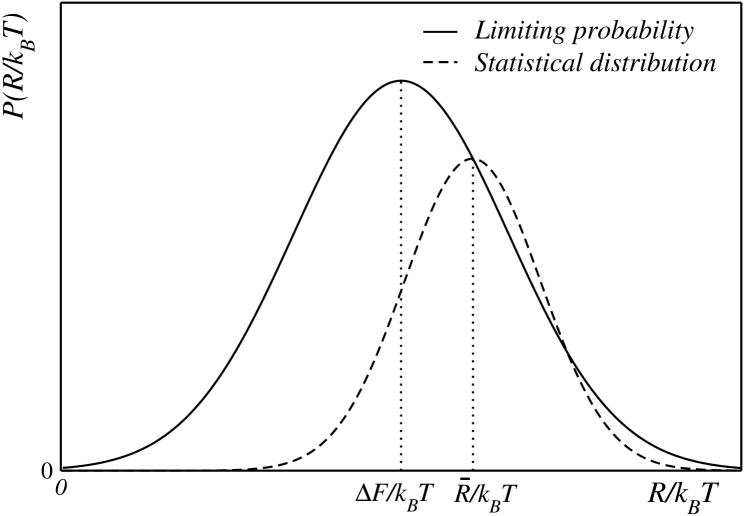
Figure 1:

References

- (1) A. Pais, Subtle is the Lord… (Oxford, 1982), Chapter II.
- (2) E. G. D. Cohen, Physica A 305, 19 (2002).
- (3) E. G. D. Cohen, PRANAMA J. Phys. 64, 635 (2005).
- (4) J. Liphart, S. Dumont, S. B. Tinoco I Jr and C. Bustamante, Science 296, 1832 (2002).
- (5) C. Storm, J. J. Pastore, F. C. MacKintosh, T. C. Lubensky, P. A. Janmey, Nature 435, 191(2005)
- (6) J. M. Ortíz de Zárate, J.V. Sengers, Hydrodynamic fluctuations in fluids and fluid mixtures (Elsevier, Amsterdam, 2006).
- (7) S. R. de Groot and P. Mazur, Non-equilibrium thermodynamics (Dover, New York, 1984).
- (8) D. Reguera, J. M. G. Vilar, J. M. Rubí, J. Phys. Chem. B 109, 21502 (2006).
- (9) J. M. G. Vilar and J. M. Rubí, Proc. Natl. Acad. Sci. 98, 11081 (2001).
- (10) G. Gallavotti and E. G. D. Cohen, Phys. Rev. Lett. 74, 2694 (1995).
- (11) C. Jarzynski, Phys. Rev. Lett. 78, 2690 (1997).
- (12) G. E. Crooks, Phys. Rev. E 60, 2721 (1999).
- (13) E. G. D. Cohen and D. Mauzerall, J. Stat. Mech. P07006 (2004).
- (14) R. Balescu, Equilibrium and Non-equilibrium Statistical Mechanics (Wiley-Interscience, NY, 1975) See also R. Balescu, Statistical Dynamics. Matter out of Equilibriu (Imperial College Press, London, 1997).
- (15) R. Zwanzig, Nonequilibrium Statistical Mechanics (Oxford, New York, 2001).
- (16) P. G. Debenedetti and F. H. Stillinger, Nature 410, 259 (2001).
- (17) E. R. Weeks and D. A. Weitz, Phys. Rev. Lett. 89, 095704 (2002).
- (18) L. D. Landau and E. M. Lifshitz, Statistical Physics (Pergamon, New York, 1988).
- (19) Benoit Palmieri and David Ronis, Phys. Rev. E 75, 011133 (2007).
- (20) H. Cramér, Mathematical Methods of Statistics (Princeton University Press, Princeton, 1946).
- (21) N.G. van Kampen, Stochastic Processes in Physics and Chemistry (North-Holland, Amsterdam, 1990).
- (22) R. Zwanzig, J. Chem. Phys. 22, 1420 (1954).
- (23) Steve Pressé and Robert Silbey, J. Chem. Phys. 124, 054117 (2006).
- (24) A. Papoulis, Probability, stochastic variables and random processes (McGraw Hill, Singapore, 1991).
- (25) Kerson Huang, Statistical Mechanics (John Wiley & Sons, 1987), Chapter 6.
- (26) R.K. Pathria, Statistical Mechanics (Pergamon Press, 1988), Chapter 2.
- (27) T. L. Hill, Thermodynamics of Small Systems (Dover, New York, 2002), Chapter 1.
- (28) Owen G. Jepps, Gary Ayton, and Denis J. Evans, Phys. Rev. E 62, 4757 (2000).
- (29) Gerald Rickayzen and Jack G. Powles, J. Chem. Phys. 114, 4333 (2001).
- (30) Hans Henrik Rugh, Phys. Rev. Lett 78, 772 (1997).
- (31) Chris Jarzynski, J. Stat. Mech. P09005 (2004).
- (32) E.G.D. Cohen and D. Mauzerall, Molec. Phys. 103, 2923 (2005).
- (33) A. Katchalski, P. F. Curran, Nonequilibrium thermodynamics in biophysics (Harvard, Cambridge, 1975).
- (34) A. Pérez-Madrid, J. Stat. Mech. P09015 (2006).
- (35) A. Pérez-Madrid, J. Chem. Phys. 123, 204108 (2005).
- (36) A. Pérez-Madrid, Physica A 339, 339 (2004).
- (37) Jean Pierre Hansen, Ian R. McDonald, Theory of simple liquids (Academic Press, London, 1986).
- (38) A. Pérez-Madrid, Physica A 378, 299 (2007).