Correlated multi-asset portfolio optimisation
with transaction cost

Abstract

We employ perturbation analysis technique to study multi-asset portfolio optimisation with transaction cost. We allow for correlations in risky assets and obtain optimal trading methods for general utility functions. Our analytical results are supported by numerical simulations in the context of the Long Term Growth Model.

1 Introduction

In recent years, the study of portfolio optimisation under non-zero transaction cost has received its due attention (Davis & Norman 1990; Atkinson & Wilmott 1995; Morton & Pliska 1995; Akian et al. 1996; Atkins & Dyl 1997; Atkinson & Al-Ali 1997; Atkinson et al. 1997; Atkinson & Mokkhavesa 2001, 2003, 2004; Mokkhavesa & Atkinson 2002; Chellathurai & Draviam 2005). In the literature, it is found that the incorporation of transaction fees into the model introduces a no-transaction region around the original optimal curve, surrounded by purchase and sale regions (cf. figure 1). Most of previous work focused on having only one risky asset (stock) and one risk-free asset (bond), except the study by Atkinson and Mokkhavesa (2004) in which portfolio with multiple risky assets is analysed. In this work, the authors are able to obtain the optimal investment strategy with the assumption that the risky assets are uncorrelated. Here, we go beyond this restriction and consider correlated risky assets. By assuming that the purchase and sale boundaries are of an equal distance away from the optimal curve, we obtain analytical expressions for the optimal trading strategy for general utility functions. We further support our analytical results with numerical simulations in the context of the Long Term Growth Model.

The plan of the paper is as follows: In §2, we will consider portfolio optimisation without transaction costs, thereby introduce the dynamic programming method employed. We will then consider trading with transaction cost in §3. The details of our simulation method in support of our analytical results are given in 4. For reference, the expressions for the derivatives of the value function in terms of the expansion parameter are given in 4.

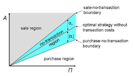
Figure 1: A schematic diagram depicting the optimal trading strategy for the long term growth model. The optimal holding of the risky asset, $A^{*}(\propto\Pi)$, is shown by the red curve. The sale-no-transaction boundary is given by $(A^{*}+\alpha_{+})$ and the purchase-no-transaction boundary is given by $(A^{*}+\alpha_{-})$ where $\alpha_{-}<0$ (cf. equation 11). In this work, we assume that $\alpha_{+}=-\alpha_{-}$.

2 Trading without transaction costs

We consider a market with investment opportunities on $n$ stocks and a risk free bond, and we let $A_{i}(t)$, $B(t)$ and $\Pi(t)\equiv B(t)+\sum_{i=1}^{n}A(t)$ be the values held in stock $i$, the value held in risk free bond and the total wealth at time $t$ respectively. We assume that $A_{i}(t)$ follows a geometric Brownian motion with growth rate $\mu_{i}$ and volatility $\sigma_{i}$, and the risk free bonds, $B$, compounds continuously with risk free rate $r$. The volatilities $\sigma_{i}$, growth rates $\mu_{i}$ and interest rate $r$ are assumed to be constant. Cash generated or needed from the purchase or sale of stocks is immediately invested or withdrawn from the risk free bonds. In the absence of transaction costs, the problem is easily solved without recourse to perturbation analysis and this section will serve to familiarise the readers with the use of dynamic programming method in this optimisation problem.

The market model equations are represented by the followings:

$${\rm d}A_{i} = \mu_{i}A_{i}{\rm d}t+\sigma_{i}A_{i}{\rm d}X_{i}\ ,\ \ i=1,\cdots,n$$

$${\rm d}B = rB{\rm d}t=r\left(\Pi-\sum^{n}_{i=1}A_{i}\right){\rm d}t$$

$${\rm d}\Pi = rB{\rm d}t+\sum^{n}_{i=1}\mu_{i}A_{i}{\rm d}t+\sum^{n}_{i=1}\sigma_{i}A_{i}{\rm d}X_{i}\ ,$$ (1)

where $X_{i}$ , $i=1,\ldots,n$, are Weiner processes whose correlations, $-1\leq\rho_{ij}\leq 1$, are assumed constant. At time $t=0$, an investor has an amount $\Pi(t=0)$ of resources and the problem is to allocate investments over the time horizon $t\in[0,T]$, so as to maximise the following expectation value:

$${\mathbf{E}}\left[F(\Pi(T))+\int_{0}^{T}I(\Pi(t^{\prime}))dt^{\prime}\right]\ .$$

The functions $I$ and $F$ can represent anything from utility to the year end bonus of the trader. For example, if we assume that $I=0$ and $F(\Pi(T))=\log(\Pi(T))$, then the opimisation problem constitutes the Long Term Growth Model and the goal would then be to optimise the logarithm of the final wealth. To make financial sense, we will assume that the utility functions are increasing and concave down, i.e.,

$$\frac{\partial I}{\partial\Pi}\geq 0\ \ \ \ \ \ \frac{\partial^{2}I}{\partial\Pi^{2}}\leq 0$$ , (2)

$$\frac{\partial F}{\partial\Pi}\geq 0\ \ \ \ \ \ \frac{\partial^{2}F}{\partial\Pi^{2}}\leq 0\ .$$ , (3)

We restate the optimisation problem in dynamic programming form by first defining the optimal expected value function, $J(\Pi,t)$:

$$J(\Pi,t)\equiv\max_{A_{i}}{\mathbf{E}}_{t}\left[F(\Pi)+\int_{t}^{T}I(\Pi(t^{\prime}))d{t^{\prime}}\right]\ .$$ (4)

We now apply the Bellman Principle and Itô’s Lemma to the above value function to obtain the following Hamilton-Bellman-Jacobi equation (Kamien 1991):

$$0 = \max_{A_{1},\ldots,A_{n}}\Bigg{[}I+\frac{\partial J}{\partial t}+r\left(\Pi-\sum^{n}_{i=1}A_{i}\right)\frac{\partial J}{\partial\Pi}$$ (5)

$$+\sum^{n}_{i=1}\mu_{i}A_{i}\frac{\partial J}{\partial\Pi}+\frac{1}{2}\sum^{n}_{i,j=1}\Omega_{ij}A_{i}A_{j}\frac{\partial^{2}J}{\partial\Pi^{2}}\Bigg{]}\ ,$$

with the boundary condition $J(\Pi,T)=F(\Pi(T))$. In the above equation, $\Omega_{ij}\equiv\sigma_{i}\sigma_{j}\rho_{ij}$ is the standard covariance matrix, and $A_{i}$ act as the control parameters in the context of dynamic programming.

In matrix notation, we can rewrite equation (5) as

$$0=\max_{A}\left[J_{t}+I+r\Pi J_{\Pi}+(\hat{\mu}\cdot A)J_{\Pi}+\frac{1}{2}(A\cdot\Omega A)J_{\Pi\Pi}\right]\ .$$ (6)

where symbols without an index denote the corresponding vectors (e.g. $A=(A_{1},\ldots,A_{n})^{T}$). We have also introduced a new vector $\hat{\mu}$, which is defined to be $(\mu_{1}-r,\ldots,\mu_{n}-r)^{T}$.

By differentiating equation (6) with respect to $A$, one obtains as the solution to the HBJ Equation:

$$\frac{\partial J}{\partial\Pi}\hat{\mu}+\frac{\partial^{2}J}{\partial\Pi^{2}}\Omega A=0\ .$$ (7)

Therefore, the optimal portfolio corresponds to:

$$A^{*}=-\frac{\partial J}{\partial\Pi}\left(\frac{\partial^{2}J}{\partial\Pi^{2}}\right)^{-1}\Omega^{-1}\hat{\mu}\ .$$ (8)

2.1 Example: the Long Term Growth Model

In this model, our aim is to maximize ${\mathbf{E}}[\log\Pi(T)]$. The value function is thus

$$J(\Pi,t)=\max_{A}{\mathbf{E}}_{t}[\log(\Pi(T))]\ .$$ (9)

such that $J(\Pi,T)=\log(\Pi(T))$. This boundary condition together with the differential equation obtained by substituting equation (8) into equation (6) implies that

$$J(\Pi,t)=\log\Pi+\left(r+\frac{1}{2}\hat{\mu}\cdot\Omega^{-1}\hat{\mu}\right)(T-t)\ .$$ (10)

The optimal portfolio from equation (8) is therefore given by:

$$A^{*}=\Pi\Omega^{-1}\hat{\mu}\ .$$ (11)

For the case of having two-risky assets, the optimal portfolio corresponds to having $B^{*}=q\Pi$ with $q\equiv 1-{\rm Tr}[\Omega^{-1}\hat{\mu}]$, and $A_{i}^{*}=p_{i}\Pi$ with $p_{i}\equiv[\Omega^{-1}\hat{\mu}]_{i}$. By the Itô’s lemma, we have

$${\rm d}(\log\Pi)=\left(rq+\mu_{1}p_{1}+\mu_{2}p_{2}-\frac{\beta^{2}}{2}\right){\rm d}t+\beta{\rm d}X$$ (12)

where

$$\beta=\sqrt{\sigma_{1}^{2}p_{1}^{2}+2\sigma_{1}\sigma_{2}p_{1}p_{2}\rho_{12}+\sigma_{2}^{2}p_{2}^{2}}\ .$$ (13)

The optimal expected payoff in this model is therefore:

$${\mathbf{E}}[\log(\Pi(T))]={\mathbf{E}}[\log(\Pi(0))]+\left(rq+\mu_{1}p_{1}+\mu_{2}p_{2}-\frac{\beta^{2}}{2}\right)T\ .$$ (14)

We now consider a two-risky-asset market model. With the model parameters given in 4, the optimal stock holdings in this case are $A_{1}^{*}=0.067\times\Pi$ and $A_{2}^{*}=0.467\times\Pi$ (cf. equation (11)). The performances of this optimal trading strategy based on our analytical expression in equation (14) and our numerical simulations (cf. 4 for details of simulation method) are given in figure 2. If the correlation in the risky assets is ignored, the optimal portfolio becomes: $A_{1}^{*}=0.3\times\Pi$ and $A_{2}^{*}=0.5\times\Pi$. The corresponding performance is shown to be sub-optimal in figure 2.

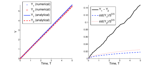
Figure 2: Analytical and simulation results for the two-risky-asset market with model parameters given in 4. Left plot: $Y_{1}\equiv\langle\log(\Pi(T))\rangle$ denotes the performance of the optimal trading strategy, while $Y_{2}$ denotes the performance of the sub-optimal strategy obtained with the correlation between the two risky assets ignored. Right plot: The plots of $(Y_{1}-Y_{2})$ and the standard errors of the means for $Y_{1}$ and $Y_{2}$ versus time based on our simulations. Note that $S=4000$ is the number of samples in the simulations.

3 Trading with transaction cost

We will now include transaction cost into our discussion. As the transaction cost usually amounts to a small percentage ($\sim 0.5\%$) of the total transaction, we employ perturbation method to analyse this optimisation problem with the transaction cost as the expansion parameter. By keeping track of the first few lowest order terms, we will derive the first order correction to the optimal trading strategy determined under no transaction cost.

We assume that the transaction fee is proportional to the asset under transaction and the proportionality constant is denoted by $k$. Note that we again define the total wealth, $\Pi$, as

$$\Pi=B+\sum_{i=1}^{n}A_{i}\ .$$ (15)

The market model equations in this case are:

$${\rm d}B = rB{\rm d}t-(1+k){\rm d}L_{i}(t)+(1-k){\rm d}M_{i}(t)$$

$$= r\left[\Pi-(1-k)\sum^{n}_{i=1}A_{i}\right]{\rm d}t-(1+k){\rm d}L_{i}(t)+(1-k){\rm d}M_{i}(t)$$

$${\rm d}A_{i} = \mu_{i}A_{i}{\rm d}t+{\rm d}L_{i}(t)-{\rm d}M_{i}(t)+\sigma_{i}A_{i}{\rm d}X_{i}\ ,\ \ i=1,\cdots,n$$

$${\rm d}\Pi = r\Pi+(1-k)\sum^{n}_{i=1}\Big{(}-rA_{i}{\rm d}t+\mu_{i}A_{i}{\rm d}t+\sigma_{i}A_{i}{\rm d}X_{i}\Big{)}$$ (16)

$$-k\sum^{n}_{i=1}\Big{(}{\rm d}L_{i}(t)+{\rm d}M_{i}(t)\Big{)}$$

where $L_{i}(t)$ and $M_{i}(t)$ represent the cumulative purchase and cumulative sale of assets $A_{i}$ during the time interval $[0,T]$. The optimal expected value function $J(\Pi,A,t)$ is as before:

$$J(\Pi,A,t)=\max_{L_{i},M_{i}}{\mathbf{E}}\left[F(\Pi(T))+\int_{t}^{T}I(\Pi({t^{\prime}}))d{t^{\prime}}\right]\ ,$$ (17)

and the corresponding HBJ equation is (Kamien 1991):

$$0 = \max_{L_{i},M_{i}}\Bigg{\{}I+\frac{\partial J}{\partial t}+\sum^{n}_{i=1}\left(\mu_{i}A_{i}+\frac{{\rm d}L_{i}}{{\rm d}t}-\frac{{\rm d}M_{i}}{{\rm d}t}\right)\frac{\partial J}{\partial A_{i}}$$ (18)

$$+\left[r\left(\Pi-\sum^{n}_{i=1}A_{i}\right)+\sum^{n}_{i=1}\left(\mu_{i}A_{i}-k\frac{{\rm d}L_{i}}{{\rm d}t}-k\frac{{\rm d}M_{i}}{{\rm d}t}\right)\right]\frac{\partial J}{\partial\Pi}$$

$$+\sum^{n}_{i,j=1}\Omega_{ij}A_{i}A_{j}\left(\frac{1}{2}\frac{\partial^{2}J}{\partial A_{i}\partial A_{j}}+\frac{1}{2}\frac{\partial^{2}J}{\partial\Pi^{2}}+\frac{\partial^{2}J}{\partial A_{i}\partial\Pi}\right)\Bigg{\}}\ .$$

Here, $L_{i}$ and $M_{i}$ are the control parameters from the dynamics programming perspective.

3.1 Three regions

By isolating terms involving ${\rm d}L$ or ${\rm d}M$ separately in equation (18), we arrive at three separate cases:

Case 1: $\frac{\partial J}{\partial A_{i}}-k\frac{\partial J}{\partial\Pi}<0$ and $-\frac{\partial J}{\partial A_{i}}-k\frac{\partial J}{\partial\Pi}\geq 0$.
In this case, the maximum in equation (18) is achieved by choosing ${\rm d}L_{i}=0$ and ${\rm d}M_{i}=\infty$, which is equivalent to selling at maximum rate.

Case 2: $\frac{\partial J}{\partial A_{i}}-k\frac{\partial J}{\partial\Pi}\geq 0$ and $-\frac{\partial J}{\partial A_{i}}-k\frac{\partial J}{\partial\Pi}\leq 0$.
In this case, the maximum is achieved by choosing ${\rm d}L_{i}=\infty$ and ${\rm d}M_{i}=0$, which is equivalent to buying at maximum rate.

Case 3: $\frac{\partial J}{\partial A_{i}}-k\frac{\partial J}{\partial\Pi}<0$ and $-\frac{\partial J}{\partial A_{i}}-k\frac{\partial J}{\partial\Pi}<0$.
In this case, the maximum is achieved by choosing ${\rm d}L_{i}=0$ and ${\rm d}M_{i}=0$, which indicates that no transactions are needed.

We note that it is not possible to have $\frac{\partial J}{\partial A_{i}}-k\frac{\partial J}{\partial\Pi}$ and $-\frac{\partial J}{\partial A_{i}}-k\frac{\partial J}{\partial\Pi}$ be both greater than zero as we assume that $J$ is an increasing function of $\Pi$. This can be broadly interpreted as more wealth cannot decrease the value function from the trader’s point of view.

With the above consideration, the optimal trading strategy can be seen to be partitioned into three separate regions: sale, purchase and no-transaction regions (cf. figure 1). In other words, if the portfolio is in the sale (purchase) region, the optimal strategy is to sell (buy) stocks until the portfolio is at the no-transaction region boundary, and thus bring the portfolio back into the no-transaction region. Inside the no-transaction region, ${\rm d}L$ and ${\rm d}M$ are identically zero and hence $J$ satisfies the HBJ equation with $k=0$.

3.2 Continuity and optimality assumptions

To make progress with our analysis, we will assume that the optimal value function, $J$, is everywhere continuous and that its derivatives are also continuous. We call the latter the optimality assumption. The validities of these assumptions are discussed in Morton & Pliska (1996) and Whalley & Wilmott (1997).

We now restrict ourselves to one risky asset for notational convenience. Suppose that the point $(\Pi,A,t)$ is inside the sale region, when a very small quantity of assets, $h$ is sold, the risk-free bond increases by the amount $h(1-k)$, while the whole portfolio value is reduced by $kh$. As $h\rightarrow 0$, the value function $J$ must be the same after the sale (the continuity assumption), we therefore have

$$\lim_{h\rightarrow 0}J(\Pi+kh,A,t) = \lim_{h\rightarrow 0}J(\Pi,A-h,t)$$ (19)

$$\lim_{h\rightarrow 0}k\frac{J(\Pi+kh,A,t)-J(\Pi,A,t)}{kh} = \lim_{h\rightarrow 0}\frac{J(\Pi,A-h,t)-J(\Pi,A,t)}{h}$$ (20)

$$k\frac{\partial J}{\partial\Pi} = -\frac{\partial J}{\partial A}\ .$$ (21)

By a similar argument, we can conclude that inside the purchase region, we have

$$k\frac{\partial J}{\partial\Pi}=\frac{\partial J}{\partial A}\ .$$ (22)

By applying again the same argument to equations (21) and (22) with the use of the optimality assumption, we have that in the sale region and at the sale-no-transaction boundary:

$$\frac{\partial^{2}J}{\partial A_{i}^{2}}=-k\frac{\partial J}{\partial A_{i}\partial\Pi}\ ;$$ (23)

and in the purchase region and at the purchase-no-transaction boundary:

$$\frac{\partial^{2}J}{\partial A_{i}^{2}}=k\frac{\partial J}{\partial A_{i}\partial\Pi}\ .$$ (24)

Inside the no-transaction region, the value function, $J$, must satisfy equation (18) with ${\rm d}L={\rm d}M=0$, i.e.,

$$0 = I+\frac{\partial J}{\partial t}+\sum^{n}_{i=1}\mu_{i}A_{i}\frac{\partial J}{\partial A_{i}}+\left[r\left(\Pi-\sum^{n}_{i=1}A_{i}\right)+\sum^{n}_{i=1}\mu_{i}A_{i}\right]\frac{\partial J}{\partial\Pi}$$ (25)

$$+\sum^{n}_{i,j=1}\Omega_{ij}A_{i}A_{j}\left(\frac{1}{2}\frac{\partial^{2}J}{\partial A_{i}\partial A_{j}}+\frac{1}{2}\frac{\partial^{2}J}{\partial\Pi^{2}}+\frac{\partial^{2}J}{\partial A_{i}\partial\Pi}\right)\ .$$

These equalities are to be supplemented by the boundary condition at $t=T$: $J(\Pi,A,T)=F(\Pi)$.

3.3 Perturbative expansion and order matching

We now redefine the $A_{i}$ coordinate as $A_{i}=A^{*}_{i}(\Pi,t)+k^{1/3}\alpha_{i}$, where $A^{*}_{i}$ is the optimal value of stock $i$ held when $k$ tends to zero, and introduce the modified value function, $H$, such that $H(\Pi,\alpha,t)={J}(\Pi,A,t)$. In 4, we display the various derivatives of $J$ in terms of $H$ and $\alpha$.

We further expand $H(\Pi,\alpha,t)$ in powers of $k^{1/3}$ as:

$$H_{0}(\Pi,\alpha,t)+k^{1/3}H_{1}(\Pi,\alpha,t)+k^{2/3}H_{2}(\Pi,\alpha,t)$$ (26)

$$+ kH_{3}(\Pi,\alpha,t)+k^{4/3}H_{4}(\Pi,\alpha,t)+{\cal O}(k^{5/3})\ .$$

The reason for expanding $H$ and $A_{i}$ in powers of $k^{1/3}$ is out of necessity and has previously been studied in the literature (Atkinson & Wilmott 1995, Rogers 2004).

We will from now on keep track of the expression up to the first non-trivial correction: ${\cal O}(k^{5/3})$. By matching the orders of $k$, equations (21) and (22) at the sale-no-transaction boundary (corresponds to the + sign in $\pm$) and at the purchase-no-transaction boundary (corresponds to the $-$ sign in $\pm$) become:

$$0 = \frac{\partial H_{m}}{\partial\alpha_{i}}\ \ \ ,\ \ \ 0\leq m\leq 2$$ (27)

$$0 = \frac{\partial H_{3}}{\partial\alpha_{i}}\pm\left(-\sum_{j=1}^{n}\frac{\partial A^{*}_{j}}{\partial\Pi}\frac{\partial H_{0}}{\partial\alpha_{j}}\right)$$ (28)

$$0 = \frac{\partial H_{4}}{\partial\alpha_{i}}\pm\frac{\partial H_{0}}{\partial\Pi}\pm\left(-\sum_{j=1}^{n}\frac{\partial A^{*}_{j}}{\partial\Pi}\frac{\partial H_{1}}{\partial\alpha_{j}}\right)\ ,$$ (29)

and equations (23) and (24) become:

$$0 = \frac{\partial^{2}H_{m}}{\partial\alpha_{i}^{2}}\ \ \ ,\ \ \ 0\leq m\leq 2$$ (30)

$$0 = \frac{\partial^{2}H_{3}}{\partial\alpha_{i}^{2}}\pm\left(-\sum_{j=1}^{n}\frac{\partial A_{j}^{*}}{\partial\Pi}\frac{\partial^{2}H_{0}}{\partial\alpha_{j}^{2}}\right)$$ (31)

$$0 = \frac{\partial^{2}H_{4}}{\partial\alpha_{i}^{2}}\pm\frac{\partial^{2}H_{0}}{\partial\alpha_{i}\partial\Pi}\pm\left(-\sum_{j=1}^{n}\frac{\partial A_{j}^{*}}{\partial\Pi}\frac{\partial^{2}H_{1}}{\partial\alpha_{j}^{2}}\right)\ .$$ (32)

Inside the no-transaction region, after expanding $H$ according to equation (26) and collecting terms of the same order in $k$, we arrive at the following conditions:

1. ${\cal O}(k^{-2/3})$ Equation: ${\cal D}H_{0}=0$, where ${\cal D}$ is an operator defined as $\sum^{n}_{i,j=1}D_{ij}\partial^{2}_{\alpha_{i}\alpha_{j}}$ with

   $$D_{ij}\equiv\frac{1}{2}\frac{\partial A^{*}_{i}}{\partial\Pi}\frac{\partial A^{*}_{j}}{\partial\Pi}\sum_{h,l=1}^{n}\Omega_{hl}A^{*}_{h}A^{*}_{l}+\frac{1}{2}\Omega_{ij}A^{*}_{i}A^{*}_{j}-\frac{\partial A^{*}_{i}}{\partial\Pi}\sum_{h=1}^{n}\Omega_{ih}A^{*}_{i}A^{*}_{h}$$ (33)

2. ${\cal O}(k^{-1/3})$ Equation: ${\cal D}H_{1}=0$.

3. ${\cal O}(1)$ Equation: ${\cal D}H_{2}=-{\cal{M}}H_{0}$, where ${\cal{M}}$ is an operator defined as

   $$\partial_{t}+I+r\left(\Pi-\sum^{n}_{i=1}A^{*}_{i}\right)\partial_{\Pi}+\sum^{n}_{i=1}\mu_{i}A^{*}_{i}\partial_{\Pi}+\frac{1}{2}\sum_{i,j=1}^{n}\Omega_{ij}A^{*}_{i}A^{*}_{j}\partial^{2}_{\Pi\Pi}\ .$$ (34)

4. ${\cal O}(k^{1/3})$ Equation: ${\cal D}H_{3}=-\sum^{n}_{i=1}\alpha_{i}\partial_{A_{i}}({\cal{M}}H_{0})-{\cal{M}}H_{1}$.

5. $O(k^{2/3})$ Equation: ${\cal D}H_{4}=-\frac{1}{2}\frac{\partial^{2}H_{0}}{\partial\Pi^{2}}\sum^{n}_{i,j=1}\Omega_{ij}\alpha_{i}\alpha_{j}-{\cal{M}}H_{2}$.

Combining the ${\cal O}(k^{-2/3})$ equation with equations (27) and (30) when $m=0$, one finds that $H_{0}$ is independent of $\alpha$. Combining the ${\cal O}(k^{-1/3})$ with equations (27) and (30) when $m=1$ shows that $H_{1}$ is independent of $\alpha$. Combining the ${\cal O}(1)$ equation with equations (27) and (30) when $m=2$ shows that $H_{2}$ is independent of $\alpha$. The ${\cal O}(k^{1/3})$ equation together with equations (28) and (31) imply that $H_{3}$ is independent of $\alpha$. In summary, by matching the coefficients of the various orders in $k$, we determine that $H_{0},H_{1},H_{2},H_{3}$ are independent of $\alpha$.

Without loss of generality, we focus on the first asset and let $\alpha_{1+}$ denotes the width of the purchase-no-transaction boundary, and $\alpha_{1-}$ the width of the sale-no-transaction boundary (cf. figure 1). From equations (29) and (30), we find that at the boundary $A^{*}+\alpha_{1-}$:

$$\frac{\partial H_{4}}{\partial\alpha_{1}}+\frac{\partial H_{0}}{\partial\Pi} = 0$$ (35)

$$\frac{\partial^{2}H_{4}}{\partial\alpha_{1}^{2}} = 0\ ,$$ (36)

and at boundary $A^{*}+\alpha_{1+}$, we have:

$$\frac{\partial H_{4}}{\partial\alpha_{1}}-\frac{\partial H_{0}}{\partial\Pi} = 0$$ (37)

$$\frac{\partial^{2}H_{4}}{\partial\alpha_{1}^{2}} = 0\ .$$ (38)

As we have established that $H_{0}$ and $H_{2}$ are independent of $\alpha$, with the ${\cal O}(k^{2/3})$ equation, we can conclude that $H_{4}$ has the following general form:

$$H_{4}(\Pi,\alpha,t)=\sum_{j=0}^{4}h_{j}(\Pi,\alpha_{\bar{1}},t)\alpha_{1}^{j}\ ,$$ (39)

where $\alpha_{\bar{1}}$ denotes the set $\{\alpha_{m}:m>1\}$. In other words, $H_{4}$ is a polynomial in $\alpha_{1}$ with a degree of at most four. We now make the simplifying assumption that $\alpha_{+}=-\alpha_{-}$. This is equivalent to saying that the transaction (buy or sell) boundaries are of the same distance away from the unperturbed optimal curve. We note that this assumption is proved to be true in the case of having uncorrelated risky assets (Atkinson and Mokkhavesa 2004). With the assumption of equal magnitude, we can conclude that $h_{3}=0$ at the boundaries by subtracting equation (36) from equation (38). In particular, we have

$$6h_{4}\alpha_{+}^{2}+h_{2}=0\ .$$ (40)

By summing equations (35) and (37), we can further determine that $h_{1}=0$ at the boundaries. By subtracting equation (35) from equation (37), we conclude that $\alpha_{1+}$ satisfies:

$$-\frac{\partial H_{0}}{\partial\Pi}=4h_{4}\alpha_{1+}^{3}+2h_{2}\alpha_{1+}\ .$$ (41)

Substituting equation (40) into equation (41), we obtain

$$\alpha_{1+}^{3}=\frac{1}{8h_{4}}\frac{\partial H_{0}}{\partial\Pi}\ .$$ (42)

To calculate $h_{4}$, we invoke the ${\cal O}(k^{2/3})$ equation: By comparing the coefficient of the $\alpha_{1}^{2}$ term on both sides, we find that:

$$h_{4}=-\frac{\sigma^{2}_{1}}{24D_{11}}\frac{\partial^{2}H_{0}}{\partial\Pi^{2}}\ .$$ (43)

So finally, $\alpha_{1\pm}$ can be expressed as:

$$\alpha_{1\pm}^{3}=\mp\frac{3D_{11}}{\sigma^{2}_{1}}\frac{\partial H_{0}}{\partial\Pi}\left(\frac{\partial^{2}H_{0}}{\partial\Pi^{2}}\right)^{-1}\ ,$$ (44)

where $H_{0}$ is the optimal value function when transaction cost is absent.

In general, denoting the trading boundary for stock $i$ by $\alpha_{i+}$, we have the following general expression for the widths of the trading boundaries:

$$\alpha_{i+}=\left|\frac{3D_{ii}}{\sigma^{2}_{i}}\frac{\partial H_{0}}{\partial\Pi}\left(\frac{\partial^{2}H_{0}}{\partial\Pi^{2}}\right)^{-1}\right|^{1/3}\ .$$ (45)

For any financial model where $H_{0}$ is known, the above equation together with equation (8) provides an analytical description of the optimal trading strategy. This is the main result of this paper.

3.4 Example: the Long Term Growth Model

According to equations 10 and 11:

$$H_{0}(\Pi,t) = \log\Pi+\left(r+\frac{1}{2}\hat{\mu}\cdot\Omega^{-1}\hat{\mu}\right)(T-t)$$ (46)

$$A^{*} = \Pi\Omega^{-1}\hat{\mu}\ .$$ (47)

Combining these with equation (33), we have

$$D_{ii} = \frac{1}{2}\frac{\partial A^{*}_{i}}{\partial\Pi}\frac{\partial A^{*}_{j}}{\partial\Pi}\sum_{h,l=1}^{n}\Omega_{hl}A^{*}_{h}A^{*}_{l}+\frac{1}{2}\Omega_{ij}A^{*}_{i}A^{*}_{j}-\frac{\partial A^{*}_{i}}{\partial\Pi}\sum_{h=1}^{n}\Omega_{ih}A^{*}_{i}A^{*}_{h}$$ (48)

$$= \Pi^{2}\left\{\frac{1}{2}(\hat{\mu}\cdot\Omega^{-1}\hat{\mu}+\sigma_{i}^{2})[\Omega^{-1}\hat{\mu}]_{i}^{2}-\hat{\mu}_{i}[\Omega^{-1}\hat{\mu}]_{i}^{2}\right\}\ .$$ (49)

The width of the boundary for stock $i$ is therefore (cf. equation (45)):

$$\Pi\left\{\frac{3k}{\sigma_{i}^{2}}\left[\frac{1}{2}(\hat{\mu}\cdot\Omega^{-1}\hat{\mu}+\sigma_{i}^{2})[\Omega^{-1}\hat{\mu}]_{i}^{2}-\hat{\mu}_{i}[\Omega^{-1}\hat{\mu}]_{i}^{2}\right]\right\}^{1/3}\ .$$ (50)

If the risky assets are uncorrelated, the expression above coincides with the result of Atkinson & Mokkkhavesa (2004).

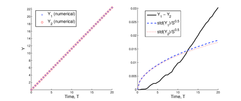
Figure 3: Simulation results for the two-risky-asset market with transaction cost. Left plot: $Y_{1}\equiv\langle\log(\Pi(T))\rangle$ denotes the performance of the optimal trading strategy, while $Y_{2}$ denotes the performance of the sub-optimal strategy obtained if the correlation between the two risky assets is ignored in the calculations for the boundary widths. Right plot: The plots of $(Y_{1}-Y_{2})$ and the standard errors of the means versus time based on our simulations. Note that $S=15000$ is the number of samples in the simulations.

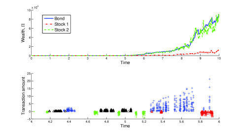
Figure 4: A particular simulation run with the optimal trading strategy in the two-risky asset model. Upper plot: the temporal evolution of values held in bond and stocks. Lower plot: The transactions performed according to the optimal trading strategy in the time interval $t\in[4,6]$. The purchases (sales) of stock $A_{1}$ are denoted by blue (green) crosses, and the purchases (sales) of stock $A_{2}$ are denoted by black (red) triangles. Note that the transaction amount is not infinitesimal only because of the discrete time evolution (tick time) in the simulations (cf.  4).

We now employ this optimal trading strategy to the two-risky-asset market considered before. The optimal curve corresponds to: $A_{1}^{*}=0.067\times\Pi$ and $A_{2}^{*}=0.467\times\Pi$ (cf. equation (11)), and according to equation (50), the boundaries widths are: $\alpha_{1+}=0.167\times k^{1/3}\Pi$ and $\alpha_{2+}=0.710\times k^{1/3}\Pi$. The performance of this strategy is shown in figure 3. If we ignore the correlation between the risky assets in calculating the boundary widths, $\alpha_{1+}$ and $\alpha_{2+}$ become $0.508\times k^{1/3}\Pi$ and $0.760\times k^{1/3}\Pi$ respectively. The trading strategy employing these boundaries together with the same optimal curve as before is shown in figure 3 and can be seen to be sub-optimal, albeit the difference is small.

In figure 4, the portfolio’s temporal evolution of a particular simulation is shown together with the transaction amounts displayed.

4 Conclusion

In conclusion, we have employed perturbation method to study multi-asset optimisation for arbitrary utility functions. By making the assumption that the sale and purchase boundaries are of the same distance away from the optimal curve, we arrived at an analytical expression for the optimal trading strategy. We have also supported our analytical results with numerical simulations in the context of the long term growth model.

Details of numerical simulation method

We consider a portfolio consisting of two risky assets and one risk-free asset. The values in the bond and risky assets are updated as follows:

$$B(t+\triangle t) = B(t)+rB(t)\triangle t$$ (51)

$$A_{1}(t+\triangle t) = A_{1}(t)+\mu_{1}A_{1}(t)\triangle t+\sigma_{1}A_{1}(t)\sqrt{\triangle t}\ z_{1}(t)$$ (52)

$$A_{2}(t+\triangle t) = A_{2}(t)+\mu_{2}A_{2}(t)\triangle t+\sigma_{2}A_{2}(t)\sqrt{\triangle t}\ z_{2}(t)$$ (53)

where $z_{1}(t)$ and $z_{2}(t)$ are random numbers drawn from the normal distribution with zero mean and a standard deviation of one, such that the correlation coefficient between $z_{1}(t)$ and $z_{2}(t)$ is $\rho_{12}$.

In the case of trading without transaction costs, the portfolio is updated after each iteration according to equation (11). When transaction costs are present, trading only occurs when the value of the risky assets are outside of the no-transaction region (cf. figure 1), i.e., if

$$A_{i}(t)\notin[A_{i}^{*}(t)+\alpha_{i+}(t),A_{i}^{*}(t)+\alpha_{i-}(t)]\ .$$ (54)

When such an event occur, the portfolio is adjusted such that $A_{i}(t)$ is moved back to the nearest boundary and the cost of transaction is subtracted from the wealth. For example, if $A_{1}(t)>A_{i}^{*}(t)+\alpha_{+}(t)$, then the portfolio is adjusted so that:

$$B(t) \rightarrow B(t)+(1-k)[A_{1}(t)-A_{1}^{*}(t)-\alpha_{1+}(t)]$$ (55)

$$A_{1}(t) \rightarrow A_{1}^{*}(t)+\alpha_{1+}(t)\ .$$ (56)

The simulations always start with a total wealth of 1 at the optimal portfolio distribution and the set of parameters employed are: $r=1,\mu_{1}=1.3,\mu_{2}=1.5,\sigma_{1}=\sigma_{2}=1,\rho_{12}=0.5,k=0.005$ and $\triangle t=5\times 10^{-5}$.

Change of variables Letting $H(\Pi,\alpha,t)=J(\Pi,A,t)$ with $A=A^{*}(\Pi,t)+k^{1/3}\alpha$, we have the following expressions for the derivative of $J$ in terms of $H$ and $\alpha$.

$$\frac{\partial J}{\partial A_{i}} = k^{-1/3}\frac{\partial H}{\partial\alpha_{i}}$$ (57)

$$\frac{\partial J}{\partial\Pi} = \frac{\partial H}{\partial\Pi}-\sum_{i=1}^{n}k^{-1/3}\frac{\partial H}{\partial\alpha_{i}}\frac{\partial A^{*}_{i}}{\partial\Pi}$$ (58)

$$\frac{\partial J}{\partial t} = \frac{\partial H}{\partial t}-\sum_{i=1}^{n}k^{-1/3}\frac{\partial H}{\partial\alpha_{i}}\frac{\partial A^{*}_{i}}{\partial t}$$ (59)

$$\frac{\partial^{2}J}{\partial A_{i}\partial A_{j}} = k^{-2/3}\frac{\partial^{2}H}{\partial\alpha_{i}\partial\alpha_{j}}$$ (60)

$$\frac{\partial^{2}J}{\partial\Pi^{2}} = \frac{\partial^{2}H}{\partial\Pi^{2}}-k^{-1/3}\sum_{i=1}^{n}\left(2\frac{\partial^{2}H}{\partial\alpha_{i}\partial\Pi}\frac{\partial A^{*}_{i}}{\partial\Pi}+\frac{\partial H}{\partial\alpha_{i}}\frac{\partial^{2}A^{*}_{i}}{\partial\Pi^{2}}\right)$$ (61)

$$+k^{-2/3}\sum_{i,j=1}^{n}\frac{\partial^{2}H}{\partial\alpha_{i}\partial\alpha_{j}}\frac{\partial A^{*}_{i}}{\partial\Pi}\frac{\partial A^{*}_{j}}{\partial\Pi}$$

$$\frac{\partial^{2}J}{\partial\Pi\partial A_{i}} = k^{-1/3}\frac{\partial^{2}H}{\partial\Pi\partial\alpha_{i}}-k^{-2/3}\sum_{j=1}^{n}\frac{\partial^{2}H}{\partial\alpha_{i}\partial\alpha_{j}}\frac{\partial A^{*}_{j}}{\partial\Pi}\ .$$ (62)

Acknowledgements

We would like to thank Colin Atkinson and Michael Giles for valuable comments. SLL thanks the Croucher Foundation, CFL thanks the Glasstone Trust (Oxford) and Jesus College (Oxford), for financial support.