Bit-Interleaved Coded Multiple Beamforming
with Imperfect CSIT

Abstract

This paper addresses the performance of bit-interleaved coded multiple beamforming (BICMB) [1], [2] with imperfect knowledge of beamforming vectors. Most studies for limited-rate channel state information at the transmitter (CSIT) assume that the precoding matrix has an invariance property under an arbitrary unitary transform. In BICMB, this property does not hold. On the other hand, the optimum precoder and detector for BICMB are invariant under a diagonal unitary transform. In order to design a limited-rate CSIT system for BICMB, we propose a new distortion measure optimum under this invariance. Based on this new distortion measure, we introduce a new set of centroids and employ the generalized Lloyd algorithm for codebook design. We provide simulation results demonstrating the performance improvement achieved with the proposed distortion measure and the codebook design for various receivers with linear detectors. We show that although these receivers have the same performance for perfect CSIT, their performance varies under imperfect CSIT.

I Introduction

It is well-known that multiple-input multiple-output (MIMO) systems enhance the throughput of wireless systems, with an increase in reliability and spectral efficiency [3], [4], [5]. While the advantages of MIMO architectures are attainable when only the receiver side knows the channel, the potential gains can be further improved when the transmitter has some knowledge of the channel, which is known as channel state information at the transmitter (CSIT). CSIT can be used to improve diversity order or array gain of a MIMO wireless system. In this work, we are interested in multi-stream precoding to achieve MIMO spatial multiplexing. In this paper “spatial multiplexing order” refers to the number of multiple symbols transmitted, as in [6]. This term is different than “spatial multiplexing gain” defined in [7]. Throughout the paper, we will employ the terminology single beamforming and multiple beamforming to refer to single- and multi-stream precoding, respectively [8], [9].

Precoders based on perfect CSIT are designed in [10], [11], [12] for many different design criteria. The majority of the designs include the channel eigenvectors which are obtained through the singular value decomposition (SVD) of the channel. It is well-known that it may not be practical to have perfect CSIT. In this paper, we will design a system with limited CSIT when the channel obeys the standard block fading (quasi-static) model. In this model, the channel may change from block to block, but remains constant during the transmission of a block. This model is commonly used in the design and simulation of broadband wireless systems.

Recently, limited CSIT feedback techniques have been introduced to achieve a performance close to the perfect CSIT case. In these, a codebook of precoding matrices is known both at the transmitter and receiver. The receiver selects the precoding matrix that satisfies a desired criterion, and only the index of the precoding matrix is sent back to the transmitter. Initial work on limited feedback systems concentrated on single beamforming where a single symbol is transmitted along a quantized version of the optimal beamforming direction. Authors of [13] analyzed single beamforming in a multi-input single-output (MISO) setting where they designed codebooks via the generalized Lloyd algorithm. The relationship between codebook design for quantized single beamforming and Grassmannian line packing was observed in [14], [15] for i.i.d. Rayleigh fading channels. This connection enabled the authors in [14], [15] to leverage the work already carried out for optimal line packing in the mathematics literature. Authors in [16] proposed a systematic way of designing good codebooks for single beamforming inspired from [17]. Rate-distortion theory tools were used in [18] to analyze single beamforming performance when the generalized Lloyd algorithm is used. Random vector quantization (RVQ) technique, where a random codebook is generated for each channel realization, was used to analyze single beamforming in an asymptotic scenario [19]. Later, results were generalized to multiple beamforming [20], [21]. The results in [20] showed that there is a relation between codebook design for multiple beamforming and Grassmannian subspace packing. However the results in [20] are specific to uncoded multiple beamforming. Most papers considered the unitary or semi-unitary constraint on the precoder since the optimal linear precoder is unitary with perfect CSIT for linear receiver architectures [8]. In such a case, it is possible to exploit the properties of unitary matrices and parameterize the optimal precoder into a set of angles to be quantized [22], [23]. hat with the

It has been shown that for a MIMO system with $N$ transmit and $M$ receive antennas, it is possible to achieve full spatial diversity of $NM$, independent of the number of streams $1\leq S\leq\min(N,M)$ transmitted over quasi-static Rayleigh flat fading channels. One possible system achieving this limit is the so-called bit-interleaved coded multiple beamforming (BICMB) [1], [2]. Design criteria for the interleaver and the convolutional encoder which guarantee full diversity and full spatial multiplexing are provided in [1], [2]. Previously, bit-interleaved coded modulation (BICM) [24], [25] was employed in single- and multi-antenna systems without utilizing CSIT [26], [27], [28], [29]. In general, BICMB requires perfect knowledge of only channel eigenvectors at the transmitter, i.e., does not need the channel gains (eigenvalues) at the transmitter. It has linear detection complexity and needs a simple soft-input Viterbi decoder. It also achieves full diversity without any adaptation for the number of streams.

In this paper, the goal is to design a limited feedback scheme for BICMB. We first deal with codeword selection criterion assuming that there is already a given codebook. We provide a new optimal distortion measure for the selection of the best precoder from the codebook. This new distortion measure is due to the non-uniqueness property of the SVD [30]. We then calculate a centroid for this new distortion measure. We analyze the performance of the proposed distortion measure for different receiver structures through extensive simulations. For comparison purposes, we first use a randomly generated codebook. Next, we utilize the generalized Lloyd’s algorithm [31] to design better codebooks. For this new codebook, we employ the minimum mean square error (MMSE) and the zero-forcing (ZF) receivers as well as a new receiver.

Notation: $N$ is the number of transmit antennas, $M$ is the number of receive antennas. The symbol $S$ denotes the total number of symbols transmitted at a time (spatial multiplexing order, in other words the total number of streams used). The superscripts $(\cdot)^{\dagger}$, $(\cdot)^{H}$, $(\cdot)^{T}$, $(\cdot)^{*}$, and the symbol $\forall$ denote the pseudoinverse, Hermitian, transpose, complex conjugate, and for-all respectively.

II System Model

In the limited feedback context, authors of [20] showed that, in their uncoded system, for both the ZF and the MMSE receiver the optimal precoder is in the form of $\mathbf{VQ}$, where is $\mathbf{V}$ is the channel right singular matrix and $\mathbf{Q}$ is any unitary matrix. This characterization enabled authors to see the direct relation between codebook design for multiple beamforming and Grassmannian subspace packing. However, as we will show, in our system, multiplication of the channel right singular matrix $\mathbf{V}$ with a general unitary matrix $\mathbf{Q}$, and employing $\mathbf{VQ}$ as the precoding matrix causes performance degradation. A new selection criterion and codebook design procedure is needed for limited feedback in BICMB.

In BICMB, the output bits of a binary convolutional encoder are interleaved and then mapped over a signal set $\chi\subseteq\mathbb{C}$ of size $|\chi|=2^{m}$ with a binary labeling map $\mu:\{0,1\}^{m}\to\chi$. We use the same interleaver that was previously employed for the perfect CSIT case in [2]. The interleaver is not unique and not necessarily the optimal one, but satisfies the design criterion and enables the system to have full diversity when perfect CSIT is available. Gray encoding is used to map the bits onto symbols. During transmission, the code sequence $\underline{c}$ is interleaved by $\pi$, and then mapped onto the signal sequence $\underline{x}\in\chi$.

Let $\mathbf{H}$ denote the quasi-static, flat fading $M\times N$ MIMO channel, where $M$ and $N$ are the number of receive and transmit antennas, respectively, and assume perfect timing, synchronization and sampling. In this paper, we assume that the transmitter employs multiple beamforming prior to the transmission of the complex baseband symbols. When $S$ symbols are transmitted at the same time, the system input-output relation between transmitted and received baseband complex symbols can be written as

$$\mathbf{y} =\mathbf{HV}_{L}\mathbf{x}+\mathbf{n}$$ (1)

where $\mathbf{x}$ is an $S\times 1$ vector of symbols to be transmitted, $\mathbf{n}$ is an $M\times 1$ additive white Gaussian noise vector whose elements have zero mean and variance $N_{0}=N/SNR$, and $\mathbf{V}_{L}$ is an $N\times S$ precoding matrix, which is dependent on the instantaneous channel realization. The total power transmitted is scaled as $N$. The channel matrix elements are modeled as i.i.d. zero-mean, unit-variance complex Gaussian random variables. Consequently, the received average signal-to-noise ratio is $SNR$.

We assume that the receiver selects a precoder matrix from a finite set of beamforming matrices and sends the index of the selected precoder through an error-free feedback link without any delay. Precoded symbols are transmitted over the channel and at the receiver a linear equalizer is used as a detector prior to the Viterbi decoder. Our aim is to investigate the effects of imperfect CSIT on the BICMB system compared to the perfect CSIT scenario and therefore, we concentrate on a linear detector followed by soft input non-iterative Viterbi decoder as in [1], [2]. In this paper we do not consider nonlinear detectors or iterative decoding techniques.

The bit interleaver of BICMB can be modeled as $\pi:k^{\prime}\to(k,s,i)$ where $k^{\prime}$ denotes the original ordering of the coded bits $c_{k^{\prime}}$, $k$ denotes the time ordering of the signals $x_{k,s}$ transmitted, $s$ denotes the subchannel used to transmit $x_{k,s}$, and $i$ indicates the position of the bit $c_{k^{\prime}}$ on the symbol $x_{k,s}$. Let $\chi_{b}^{i}$ denote the subset of all signals $x\in\chi$ whose label has the value $b\in\{0,1\}$ in position $i$. The bit metrics, i.e., $\gamma^{i}(y_{k,s},c_{k^{\prime}})$, are dependent on the receiver structure and will be revisited in Section III-D. The Viterbi decoder at the receiver makes decisions according to the rule

$$\underline{\boldsymbol{\hat{c}}}=\arg\min_{\underline{\boldsymbol{c}}\in\mathcal{C}}\sum_{k^{\prime}}\gamma^{i}(y_{k,s},c_{k^{\prime}}).$$ (2)

III Bit-Interleaved Coded Multiple Beamforming

III-A Background on SVD

As stated previously, the work in this paper depends on the fact that SVD has an invariance property under diagonal unitary transformation. We provide a formal description of this fact below [30].

Theorem 1

If $\mathbf{H}\in\mathbb{C}^{M\times N}$ has rank $k$, then it may be written in the form $\mathbf{H=U\Sigma V}^{H}$, where $\mathbf{U}$ and $\mathbf{V}$ are unitary matrices whose columns are the left and right singular vectors of $\mathbf{H}$. The matrix $\mathbf{\Sigma}=[\sigma_{ij}]\in\mathbb{R}^{M\times N}$ has $\sigma_{ij}=0$ for all $i\neq j$, and $\sigma_{11}\geq\cdots\geq\sigma_{kk}>0$, and $\sigma_{k+1,k+1}=$ $\cdots=\sigma_{qq}=0$, where $q=\min(N,M)$. The numbers $\sigma_{ii}\equiv\sigma_{i},i=1,2,\ldots,q$ are the nonnegative square roots of the eigenvalues of $\mathbf{HH}^{H}$, and hence are uniquely determined. The columns of $\mathbf{U}$ are eigenvectors of $\mathbf{H}\mathbf{H}^{H}$ and the columns of $\mathbf{V}$ are eigenvectors of $\mathbf{H}^{H}\mathbf{H}$. If $N\leq M$ and if $\mathbf{H}^{H}\mathbf{H}$ has distinct eigenvalues, then $\mathbf{V}$ is determined up to a right diagonal unitary matrix $\mathbf{D}=$ diag$(e^{j\theta_{1}},e^{j\theta_{2}},\ldots,e^{j\theta_{N}})$ with all $\theta_{i}\in[0,2\pi)$; that is, if $\mathbf{H=U}_{1}\mathbf{\Sigma}\mathbf{V}_{1}^{H}=\mathbf{U}_{2}\mathbf{\Sigma}\mathbf{V}_{2}^{H}$, then $\mathbf{V}_{2}=\mathbf{V}_{1}\mathbf{D}$.

Proof:

See [30]. ∎

The conditions of the theorem above hold for the system in this paper, and therefore there are infinitely many right singular matrices for a given channel realization. Note that when $S\leq q$ streams are transmitted, the first $S$ columns of $\mathbf{V}$, i.e., $\overline{\mathbf{V}}$, are employed. Therefore, if $\mathbf{H=U}_{1}\mathbf{\Sigma}\mathbf{V}_{1}^{H}=\mathbf{U}_{2}\mathbf{\Sigma}\mathbf{V}_{2}^{H}$, then $\overline{\mathbf{V}}_{2}=\overline{\mathbf{V}}_{1}\mathbf{D}$ and $\overline{\mathbf{U}}_{2}=\overline{\mathbf{U}}_{1}\mathbf{D}$, where $\mathbf{D}$ is any $S\times S$ diagonal unitary matrix.

III-B Selection Criteria

In this section, we assume that there exists a codebook and we wish to find a criterion to choose the best approximation to $\mathbf{V}$ from the codebook $\mathbb{V}=\{\mathbf{\hat{V}}_{i}\}_{i=1}^{C}$, where $C$ is the codebook size. One could potentially use the well-known Euclidean metric, however the property described in Theorem 1 complicates the problem.

Selection Criterion - Euclidean (SC-E) : The receiver selects $\mathbf{V}_{L}$ such that

$$\mathbf{V}_{L}=\mbox{ }\underset{\mathbf{\hat{V}}_{i}\in\mathbb{V}}{\arg\min}\mbox{ }||\mbox{ }\mathbf{V}-\mathbf{\hat{V}}_{i}\mbox{ }||_{F}^{2}.$$ (3)

This selection criterion aims to find the codebook element closest to the optimal beamforming matrix $\mathbf{V}$. It can be argued that this criterion asymptotically diagonalizes the system as the number of feedback bits goes to infinity.

However, the property in Theorem 1 makes straightforward application of (3) nonpractical. This can be explained with the aid of Figure 1. Assume that an application of SVD for a given instantiation of the $\mathbf{H}$ matrix yields a $\mathbf{V}$ matrix. Assume that when $\mathbf{V}$ is multiplied by all diagonal unitary matrices $\mathbf{D}$, one gets the set $\mathbb{S}_{\mathbf{V}}$ in Figure 1. It should be clear that the closest member of $\mathbb{V}$ to $\mathbf{V}$ is not necessarily the closest member of $\mathbb{V}$ to $\mathbb{S}_{\mathbf{V}}$. As a result, one needs to modify (3) such that the minimum distance between two sets $\mathbb{V}$ and $\mathbb{S}_{\mathbf{V}}$ can be calculated. A way to accomplish this is

$$\mathbf{V}_{L}=\mbox{ }\underset{{\mathbf{\hat{V}}_{i}\in\mathbb{V},\mathbf{D}\in\mathbb{D}}}{\arg\min}\mbox{ }||\mbox{ }\mathbf{VD}-\mathbf{\hat{V}}_{i}\mbox{ }||_{F}^{2}$$ (4)

where $\mathbb{D}$ stands for the set of all diagonal unitary matrices.

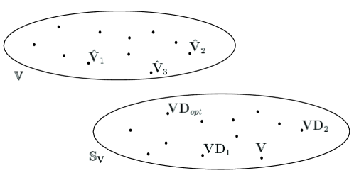
Figure 1: Sets illustrating the the codebook elements,$\mathbb{V}$, and unitary matrices from SVD, $\mathbb{S}_{\mathbf{V}}$.

Proposition 1: The minimization in (4) is equivalent to the following minimization problem

$$\mathbf{V}_{L}=\underset{\mathbf{\hat{V}}_{i}\in\mathbb{V}}{\arg\min}\mbox{ }||\mbox{ }\mathbf{VD}^{opt}-\mathbf{\hat{V}}_{i}\mbox{ }||_{F}^{2}.$$ (5)

The $k^{th}$ diagonal element of the diagonal matrix $\mathbf{D}^{opt}$ is given as

$$\theta_{k}^{opt}=-\phi_{k}\quad\quad{}k=1,2,\ldots,S$$ (6)

where $0\leq\phi_{k}<2\pi$ is the phase of $\mathbf{\hat{v}}_{ik}^{H}\mathbf{v}_{k}$ and where the vectors $\mathbf{\hat{v}}_{ik}$ and $\mathbf{v}_{k}$ correspond to the $k^{th}$ column of $\mathbf{\hat{V}}_{i}$ and $\mathbf{V}$, respectively.

Proof:

Without loss of generality, let $N\leq M$ and $S=N$ streams be used. For the other cases, the matrices are replaced by their first $S$ columns. The term to be minimized in (4) can be expressed as

$$||\mbox{ }\mathbf{VD}-\mathbf{\hat{V}}_{i}\mbox{ }||_{F}^{2}=\mbox{ } 2\textrm{tr}[\mathbf{I}]-\textrm{tr}\left[\mathbf{\hat{V}}_{i}^{H}\mathbf{VD}+(\mathbf{\hat{V}}_{i}^{H}\mathbf{VD})^{H}\right]$$ (7)

$$=\mbox{ } 2N-2\textrm{tr}\left[\Re[\mathbf{\hat{V}}_{i}^{H}\mathbf{VD}]\right]$$

$$=\mbox{ } 2N-2\Re\left[\sum\limits_{k=1}^{N}\mathbf{\hat{v}}_{ik}^{H}\mathbf{v}_{k}e^{j\theta_{k}}\right]$$ (8)

where $\mathbf{D}=$ diag$(e^{j\theta_{1}},e^{j\theta_{2}},\ldots,e^{j\theta_{N}})$, $\mathbf{\hat{v}}_{ik}$ and $\mathbf{v}_{k}$ correspond to the $k^{th}$ column of $\mathbf{\hat{V}}_{i}$ and $\mathbf{V}$, respectively. Minimizing (7) is equivalent to maximizing the second term in (8). It is easy to see that the optimal value of $\theta_{k}$ maximizing the summation in (8) is

$$\theta_{k}^{opt}=-\phi_{k}\quad\quad{}k=1,2,\ldots,N$$ (9)

where $0\leq\phi_{k}<2\pi$ is the phase of $\mathbf{\hat{v}}_{ik}^{H}\mathbf{v}_{k}=|\mathbf{\hat{v}}_{ik}^{H}\mathbf{v}_{k}|e^{j\phi_{k}}$. ∎

Proposition 1 results in the following optimal selection criterion in the Euclidean sense.

Selection Criterion - Optimal Euclidean (SC-OE) : The receiver selects $\mathbf{V}_{L}$ such that

$$\mathbf{V}_{L}=\underset{\mathbf{\hat{V}}_{i}\in\mathbb{V}}{\arg\min}\mbox{ }||\mbox{ }\mathbf{VD}^{opt}-\mathbf{\hat{V}}_{i}\mbox{ }||_{F}^{2}.$$ (10)

Note that, in (10), $\mathbf{D}^{opt}$ depends on both $\mathbf{V}$ and $\mathbf{\hat{V}}_{i}$. Employing (10), one can apply the well-known generalized Lloyd algorithm [31] to design an optimum codebook $\mathbb{V}$. The resulting codebook can then be used together with (10), as a limited-rate CSIT BICMB system. To that end, we will need centroids for the generalized Lloyd algorithm. We will calculate these new centroids in the next subsection.

III-C Codebook Design

Our codebook design is based on generalized Lloyd’s algorithm [31]. We will minimize the average distortion

$$J=E\left[\underset{\mathbf{\hat{V}}_{i}\in\mathbb{V}}{\min}\mbox{ }||\mbox{ }\mathbf{VD}^{opt}-\mathbf{\hat{V}}_{i}\mbox{ }||_{F}^{2}\right].$$ (11)

Here, the distortion measure we intend to use is

$$d(\mathbf{\hat{V}}_{i},\mathbf{V})=||\mbox{ }\mathbf{V}-\mathbf{\hat{V}}_{i}\mbox{ }||_{F}^{2}.$$ (12)

But, due to the previous discussion, we need to calculate the distortion between each $\mathbf{\hat{V}}_{i}$ and the whole set $\mathbb{S}_{\mathbf{V}}$. As a result, we employ

$$d_{1}(\mathbf{\hat{V}}_{i},\mathbf{V})=||\mbox{ }\mathbf{VD}^{opt}-\mathbf{\hat{V}}_{i}\mbox{ }||_{F}^{2}$$ (13)

due to the nonuniqueness property of SVD. We assume that $B$ bits are reserved for the limited feedback link to quantize the optimal beamforming matrix. In this algorithm, we will begin with an initial codebook of matrices $\mathbb{\tilde{V}}_{0}=\{{\mathbf{\tilde{V}}_{0,k}}\}_{k=1}^{2^{B}}$ and iteratively improve it to generate a set of matrices $\mathbb{\tilde{V}}_{m}=\{{\mathbf{\tilde{V}}_{m,k}}\}_{k=1}^{2^{B}}$ until the algorithm converges. The algorithm can be summarized by the following steps:

1) Generate a large training set of channel matrices, $\mathbf{H}(n)$ and their corresponding right singular matrices $\mathbf{V}(n)$. Let $\Psi$ be the set of all $\mathbf{V}(n)$s.

2) Generate an initial codebook of unitary matrices, $\mathbb{\tilde{V}}_{0}=\{{\mathbf{\tilde{V}}_{0,k}}\}_{k=1}^{2^{B}}$.

3) Set $m=1$.

4) Partition the set of training matrices into $P=2^{B}$ quantization regions where the $k^{th}$ region is defined as

$$\mathbb{X}_{k}=\{\mathbf{V}\in\Psi|\mbox{ }||\mbox{ }\mathbf{VD}^{opt}-\mathbf{\tilde{V}}_{m-1,k}\mbox{ }||_{F}^{2}\leq||\mbox{ }\mathbf{VD}^{opt}-\mathbf{\tilde{V}}_{m-1,l}\mbox{ }||_{F}^{2}\mbox{ }\mbox{ }\forall\mbox{ }k\neq l\}$$ (14)

5) Using the given partitions, construct a new codebook $\tilde{\mathbb{V}}_{m}$, with the $k^{th}$ beamforming matrix being

$$\mathbf{\tilde{V}}_{m,k}=\underset{\mathbf{\hat{V}}:\mbox{ }\mathbf{\hat{V}}^{H}\mathbf{\hat{V}=I}}{\arg\min}E\left[||\mbox{ }\mathbf{VD}^{opt}-\mathbf{\hat{V}}\mbox{ }||_{F}^{2}\mbox{ }|\mbox{ }\mathbf{V}\in\mathbb{X}_{k}\right].$$ (15)

6) Define

$$J_{m}=\sum\limits_{i=1}^{2^{B}}\sum\limits_{n:\mathbf{V}(n)\rightarrow\mathbf{\tilde{V}}_{m,i}}||\mbox{ }\mathbf{V}(n)\mathbf{D}^{opt}-\mathbf{\tilde{V}}_{m,i}\mbox{ }||_{F}^{2}$$ (16)

where $\mathbf{V}(n)\rightarrow\mathbf{\tilde{V}}_{m,i}$ means $\mathbf{\tilde{V}}_{m,i}=\underset{\mathbf{\hat{V}}_{j}\in\tilde{\mathbb{V}}_{m}}{\arg\min}\mbox{ }d_{1}(\mathbf{\hat{V}}_{j},\mathbf{V}(n))$ . If $(J_{m-1}-J_{m})/J_{m-1}>\epsilon$, set $m=m+1$ and go back to Step 4. Otherwise, terminate the algorithm and set the codebook $\mathbb{V}=\tilde{\mathbb{V}}_{m}$.

The optimal solution of the optimization problem in (15) gives the optimal centroid for the corresponding region. The distortion measure to be minimized can be rewritten as

$$||\mbox{ }\mathbf{VD}^{opt}-\mathbf{\hat{V}}_{i}\mbox{ }||_{F}^{2}=\mbox{ } 2N-2\textrm{tr}\left[\Re[\mathbf{\hat{V}}^{H}\mathbf{VD}^{opt}]\right]$$

$$=\mbox{ } 2N-2\Re\left[\sum\limits_{s=1}^{N}\mathbf{\hat{v}}_{s}^{H}\mathbf{v}_{s}e^{j\theta_{s}^{opt}}\right]$$

$$=\mbox{ } 2N-2\sum\limits_{s=1}^{N}|\mathbf{\hat{v}}_{s}^{H}\mathbf{v}_{s}|$$ (17)

where (17) follows by using the optimal $\theta_{s}^{opt}$ previously derived in (9). Therefore the original optimization problem in (15) can be rewritten as

$$\mathbf{\tilde{V}}_{m,k}=\underset{\mathbf{\hat{V}}:\mbox{ }\mathbf{\hat{V}}^{H}\mathbf{\hat{V}=I}}{\arg\max}E\left[\sum\limits_{s=1}^{N}|\mathbf{\hat{v}}_{s}^{H}\mathbf{v}_{s}|\mbox{ }|\mbox{ }\mathbf{V}\in\mathbb{X}_{k}\right].$$ (18)

The maximization problem above does not have a tractable analytical solution. Next, we will modify the problem to find an approximate analytical solution. Note that the expectation in (18) can be written as the sum of expectation of each term due to the linearity of the expectation operation. We will relax the unitary constraint on $\mathbf{\hat{V}}$ and replace the constraint with having unit norm columns. In this case, the modified optimization problem is equivalent to finding independent optimal vectors which maximize each expectation in (18). The individual maximization problem becomes

$$\mathbf{\tilde{e}}_{m,k}^{(i)}=\underset{\mathbf{\hat{e}}:\mbox{ }||\mathbf{\hat{e}}||_{2}^{2}=1}{\arg\max}\mbox{ }E\left[|\mathbf{\hat{e}}^{H}\mathbf{v}_{i}|\mbox{ }|\mbox{ }\mathbf{v}_{i}\in\mathbb{X}_{k}^{(i)}\right]\quad i=1,2,\ldots,N$$ (19)

where $\mathbb{X}_{k}^{(i)}$ corresponds to the space of the $i^{th}$ column of the elements in $\mathbb{X}_{k}$. The optimal solution for (19) is [32]

$$\mathbf{\tilde{e}}_{m,k}^{(i)}=\mbox{ principal eigenvector of }E\left[\mathbf{v}_{i}\mathbf{v}_{i}^{H}|\mbox{ }\mathbf{v}_{i}\in\mathbb{X}_{k}^{(i)}\right]$$ (20)

where the numerical averaging over $\mathbb{X}_{k}^{(i)}$ is substituted for expectation during codebook design. Let $\mathbf{\tilde{E}}_{m,k}$ be the matrix whose columns are found from (20), maximizing the expectation in (19) and approximating the maximization in (18). Note that this matrix is not necessarily unitary, therefore to find the centroid we will utilize Euclidean projection to find the closest unitary matrix as follows

$$\mathbf{\tilde{V}}_{m,k}=\underset{\mathbf{\hat{V}}:\mbox{ }\mathbf{\hat{V}}^{H}\mathbf{\hat{V}=I}}{\arg\min}||\mbox{ }\mathbf{\tilde{E}}_{m,k}-\mathbf{\hat{V}}\mbox{ }||_{F}^{2}.$$ (21)

The closest unitary matrix can be found in closed form as [30]

$$\mathbf{\tilde{V}}_{m,k}=\mathbf{\tilde{U}}\mathbf{\tilde{W}}^{H}$$ (22)

where $\mathbf{\tilde{E}}_{m,k}=\mathbf{\tilde{U}\tilde{\Sigma}}\mathbf{\tilde{W}}^{H}$.

The approach explained above to find the centroid in each region reduces to the optimal solution for the single beamforming case. Although it may be suboptimal for the multiple beamforming case, the centroid found from (22) enables the algorithm to have monotonic decrease in average distortion given by (11) in each iteration and to converge to a local minimum, as shown in Figure 2 for a $2\times 2$ scenario with 2 streams and 4-bit feedback.

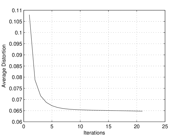
Figure 2: Average distortion for $2\times 2$ system with 4-bit feedback.

III-D The Receiver

We will first discuss the ZF and MMSE receivers and then describe a receiver based on SVD. We show in the appendix that the performance of these three decoders is the same when there is perfect CSIT.

1) ZF Receiver

When there is only limited feedback for the quantization of $\mathbf{V}$, i.e., $\mathbf{V}_{L}$ is used as the precoder, the diagonalization of the channel will be lost and with the ZF detector, the system input-output relation becomes;

$$\mathbf{r}=\mathbf{Gy}=\mathbf{x}+\mathbf{Gn}$$ (23)

where $\mathbf{G}=(\mathbf{HV}_{L})^{\dagger}=[(\mathbf{HV}_{L})^{H}(\mathbf{HV}_{L})]^{-1}(\mathbf{HV}_{L})^{H}$. In this case, we will use the following bit metrics [33],

$$\gamma^{i}(r_{k,s},c_{k^{\prime}})=\min\limits_{x\in\chi_{c_{k^{\prime}}}^{i}}\frac{|r_{k,s}-x|^{2}}{{||\mathbf{g}_{s}||}^{2}}$$ (24)

where $r_{k,s}$ is the received signal after equalization at time $k$ on the $s^{th}$ stream and $\mathbf{g}_{s}$ is the $s^{th}$ column of $\mathbf{G}^{T}$.

In the perfect CSIT case, where the channel right singular matrix $\mathbf{V}$ is perfectly known at the transmitter, the bit metrics (24) of the ZF receiver are equal to that of the optimum BICMB receiver. The proof is provided in the Appendix.

2) MMSE Receiver

MMSE detector is a superior solution to the linear detection problem which balances ISI against noise enhancement. The corresponding input-output relation is given by (23), where now $\mathbf{G}$ is given by

$$\mathbf{G}=[\mathbf{(HV}_{L})^{H}\mathbf{HV}_{L}+\sigma^{2}\mathbf{I}]^{-1}\mathbf{(HV}_{L})^{H}$$ (25)

and where $\sigma^{2}=N/SNR$ from the system model given in Section II. We will use the following bit metrics [34]

$$\gamma^{i}(r_{k,s},c_{k^{\prime}})=\min\limits_{x\in\chi_{c_{k^{\prime}}}^{i}}\frac{{W_{ss}}}{1-{W_{ss}}}\left|\frac{r_{k,s}}{{W_{ss}}}-x\right|^{2}$$ (26)

where $\mathbf{W}=[\mathbf{I}+\sigma^{2}[\mathbf{(HV_{L}})^{H}\mathbf{HV_{L}}]^{-1}]^{-1}$ and $W_{ss}$ is the $s^{th}$ diagonal element of $\mathbf{W}$.

In the perfect CSIT case, the MMSE receiver is equivalent to the optimum BICMB receiver. The proof is provided in the Appendix.

3) SVD Receiver

In the case of perfect knowledge of $\mathbf{V}$ at the transmitter, the receiver can use the $\mathbf{U}^{H}$ matrix to diagonalize the channel, where $\mathbf{H=U\Sigma V}^{H}$. In the case of limited feedback, the $\mathbf{U}^{H}$ matrix can still be used as an equalizer [22], [35]. In this section, we will provide a linear detector which performs the same as the $\mathbf{U}^{H}$ detector with lower complexity. Note that, we proposed an optimum selection criterion in (10) which is needed because of the nonuniqueness property of SVD. The optimized selection criterion aims to quantize $\mathbf{VD}^{opt}$ instead of $\mathbf{V}$. Each element of the diagonal unitary matrix $\mathbf{D}^{opt}$ can be found from (9) and it is dependent on the codebook elements and the instantaneous channel realization. From Theorem 1, it is easy to see that there is a unique matching left singular matrix for $\mathbf{VD}^{opt}$, which can be used as a detector. Therefore the corresponding linear equalizer matrix is

$$\mathbf{G}=(\mathbf{UD}^{opt})^{H}.$$ (27)

In this case, when $\mathbf{V}_{L}$ is used as a precoder at the transmitter, the baseband system input-output relation is

$$\mathbf{r} =\mathbf{GHV}_{L}\mathbf{x}+\mathbf{Gn}$$ (28)

$$=(\mathbf{D}^{opt})^{H}\mathbf{\Sigma V}^{H}\mathbf{V}_{L}\mathbf{x}+\mathbf{n^{\prime}}$$ (29)

where in (29) $\mathbf{H}$ is replaced by its SVD. Note that because $\mathbf{G}$ is a unitary transformation the noise vectors $\mathbf{n^{\prime}}$ and $\mathbf{n}$ have the same statistics. Then the input-output relation for the $s^{th}$ stream becomes

$$r_{s} =\lambda_{s}e^{-j\theta_{s}^{opt}}\sum\limits_{i=1}^{S}\mbox{ }\mathbf{v}_{s}^{H}\mathbf{v}_{L,i}x_{i}+n^{\prime}_{s}$$ (30)

$$=\lambda_{s}e^{-j\theta_{s}^{opt}}\mathbf{v}_{s}^{H}\mathbf{v}_{L,s}x_{s}+\lambda_{s}e^{-j\theta_{s}^{opt}}\sum\limits_{i=1,\mbox{ }i\neq s}^{S}\mbox{ }\mathbf{v}_{s}^{H}\mathbf{v}_{L,i}x_{i}+n^{\prime}_{s}$$ (31)

$$=\lambda_{s}|\mathbf{v}_{s}^{H}\mathbf{v}_{L,s}|x_{s}+\lambda_{s}e^{-j\theta_{s}^{opt}}\sum\limits_{i=1,\mbox{ }i\neq s}^{S}\mbox{ }\mathbf{v}_{s}^{H}\mathbf{v}_{L,i}x_{i}+n^{\prime}_{s}.$$ (32)

Note that the first term has the desired signal, the second term is interference from other streams, and the third term is noise. The transmitted symbols $x_{i}$ are typically from symmetric constellations. Therefore, the mean of $x_{i}$ is zero. As discussed previously, we normalize its variance to 1. Due to bit interleaving, $x_{i}$, $i=1,2,\ldots,S$ are uncorrelated. For a given channel realization, (32) can be written in a compact form as

$$r_{s} =\tilde{\lambda}_{s}x_{s}+\tilde{n}_{s}$$ (33)

where $\tilde{\lambda}_{s}=\lambda_{s}|\mathbf{v}_{s}^{H}\mathbf{v}_{L,s}|$ and $\tilde{n}_{s}$ is approximated as a zero-mean complex Gaussian random variable with variance $\tilde{\sigma}_{s}^{2}=\lambda_{s}^{2}\sum_{i=1,i\neq s}^{S}|\mathbf{v}_{s}^{H}\mathbf{v}_{L,i}|^{2}+N/SNR$. We determined through simulations that the Gaussian approximation is highly accurate for low and intermediate SNR values (e.g., 15 dB) or when the number of feedback bits is beyond 4. Although for large SNR (e.g., 30 dB), the approximation is less accurate, as the feedback rate increases, the accuracy loss diminishes independent of SNR. In addition, this approximation enables a very simple bit-metric calculation similar to the perfect CSIT case.

Let $\chi_{b}^{i}$ denote the subset of all signals $x\in\chi$ whose label has the value $b\in\{0,1\}$ in position $i$. The bit metrics for (33) are given by [24]

$$\gamma^{i}(r_{k,s},c_{k^{\prime}})=\min\limits_{x\in\chi_{c_{k^{\prime}}}^{i}}\frac{|r_{k,s}-\tilde{\lambda}_{s}x|^{2}}{\tilde{\sigma}_{s}^{2}}.$$ (34)

In the sequel, we will call the receiver proposed in this section as the SVD receiver. We will show in the next section that the performance of the SVD receiver is close to that of the MMSE receiver for the $2\times 2$ MIMO system. The advantage of the SVD receiver over the MMSE receiver is its relative simplicity since it avoids the matrix inversions needed in (25) and (26). One can observe that when the limited feedback rate is low, the interference term may dominate the noise term, which may result in poor performance. We emphasize that the optimum receiver with a linear detector for the limited-rate CSIT system described in the previous section is the MMSE receiver. However, the SVD receiver is a simpler one with a performance tradeoff against the MMSE receiver while consistently outperforming the ZF receiver.

IV Simulation Results

In the simulations below, the industry standard 64-state 1/2-rate (133,171) $d_{free}=10$ convolutional code is used and the constellation is 16-QAM. As in all similar work, the channel is assumed to be quasi-static and flat fading.

Figure 3 illustrates that in the case of BICMB, the precoder matrix $\mathbf{V}$ is not invariant under a general unitary matrix transformation. As discussed previously, assumption of this invariance results in the Grassmannian codebook design approach studied widely in the literature [20]. Again, as discussed previously, most of the work in the literature is for uncoded systems where invariance under a general unitary matrix transformation follows from the use of optimization criterion such as MSE, SNR, or mutual information. All curves in this figure employ BICMB with ZF receiver, while the solid ones employ the $\mathbf{V}$ matrix given by SVD of $\mathbf{H}$, those with broken lines employ $\mathbf{V}^{\prime}=\mathbf{VQ}$ where $\mathbf{Q}$ is a $2\times 2$ DFT matrix, which is unitary. Clearly, BICMB performance is not invariant under a general unitary matrix transformation.

Figure 4 shows a number of different systems to illustrate the improvement due to the new selection criterion (10). This selection criterion is compared to the one that maximizes the minimum eigenvalue ($\lambda_{min}$) of $\mathbf{HV}_{i}$. This method is employed in [20] with the ZF receiver. In order to show that there is a gain due to (10), we use the ZF receiver in our system as well. Systematic generation of codebooks [17] with a selection criterion that maximizes $\lambda_{min}$ is used for the curves with legend SC-$\lambda_{min}$ and the randomly generated codebook with the selection criterion in (5) and (6) is used for the curves with legend SC-OE. As can be seen, the performance is improved significantly with the proposed approach, and with $\lambda_{min}$ approach, the performance saturates with increasing the number of bits.

Figure 5 compares (3) and (10) employing two receiver structures: ZF and MMSE. The codebook employed is randomly generated. There is clearly a significant gain due to (10) for both receivers. In Figure 6 the performance of the SVD receiver is compared with the ZF and MMSE receivers for the $2\times 2$ scenario with 2 streams. All curves in the figures use the optimized Euclidean criterion with a randomly generated codebook. The SVD receiver, which exploits the nonuniqueness of SVD both at the transmitter and the receiver, significantly outperforms the ZF receiver and achieves a performance very close to the MMSE receiver for the 8-bit scenario. Note that, the overall complexity of the system with the SVD receiver is less than the one with the MMSE receiver. When the number of feedback bits is 8 for the $2\times 2$ case, it achieves a performance 0.25 dB close to the unquantized system.

Figure 7 shows the simulation results for various receivers in a $2\times 2$ system when the codebook is designed using the VQ algorithm discussed in Section III-C. All curves use the optimal Euclidean criterion. As seen from the figure, the performance of the randomly generated codebook (RVQ) can be significantly improved for all receivers. To illustrate, the performance of MMSE 8-bit RVQ and 6-bit VQ are very close to each other, therefore 2 bit reduction is achieved via the proposed codebook design. A similar reduction can be observed for the SVD receiver. On the other hand, for the same number of feedback bits, 2 dB performance gain is achievable for the ZF receiver. Note that there is significant performance degradation when the ZF receiver is used for both RVQ and VQ scenarios compared to the MMSE and SVD receivers.

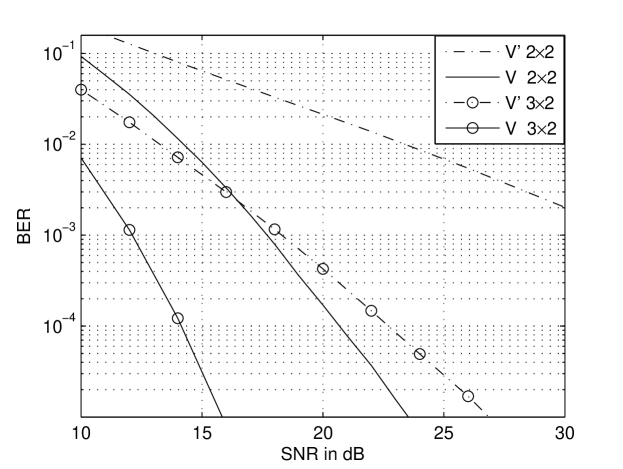
Figure 3: The precoding matrix given by SVD $\mathbf{V}$ vs. $\mathbf{V}^{\prime}=\mathbf{VQ}$ where $\mathbf{Q}$ is a DFT matrix $2\times 2$ and $3\times 2$ system with 2 streams.

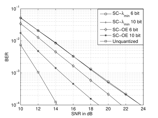
Figure 4: New selection criterion vs. $\lambda_{min}$-based selection criterion $3\times 2$ system with 2 streams.

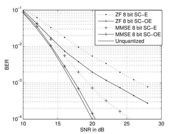
Figure 5: Comparison SC-E (3) and SC-OE (10) $2\times 2$ system with 2 streams.

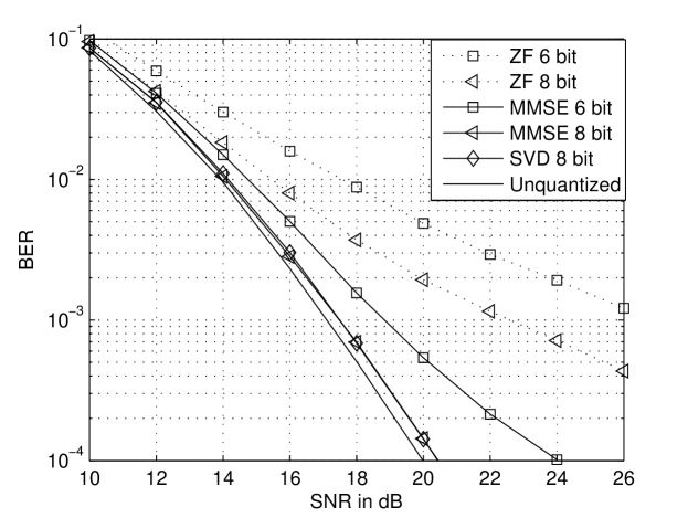
Figure 6: The SVD receiver vs. MMSE and ZF receivers using SC-OE with randomly generated codebook $2\times 2$ system with 2 streams.

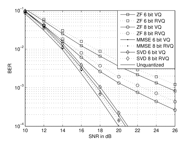
Figure 7: The SVD receiver vs. MMSE and ZF receivers with RVQ and VQ using SC-OE $2\times 2$ system with 2 streams.

V Conclusion

BICMB is a high-performance and low-complexity broadband wireless system with full spatial multiplexing and full diversity. However, the system requires perfect knowledge of the channel right singular vectors, which is not practical in a real environment.

This paper addressed the performance of BICMB with limited CSIT feedback using a codebook-based approach. We proposed a new optimal distortion measure for selecting the best precoder from a given codebook. The centroids for this distortion measure are calculated. Codebook design is performed via the generalized Lloyd algorithm based on the new distortion measure and the new centroids. We provided simulation results demonstrating the performance improvement achieved with the proposed distortion measure for various receivers with linear detectors.

Appendix A Appendix

In the perfect CSIT case, the transmitter uses the right singular matrix $\mathbf{V}$ as the precoding matrix $\mathbf{V}_{L}$. The $N\times S$ precoding matrix can be expressed as $\mathbf{V}_{L}=\mathbf{V\Phi}_{N}$, where the $N\times S$ matrix $\mathbf{\Phi}_{N}$ is used to select the first $S$ columns of $\mathbf{V}$, defined as

$$\mathbf{\Phi}_{N}=\left[\begin{array}[]{ccc}\mathbf{I}_{S}\\ \hline\cr\mathbf{0}_{N-S,S}\end{array}\right],$$

and $\mathbf{0}_{N-S,S}$ is an $(N-S)\times S$ matrix whose elements are all zeros. Therefore, the system input-output relation in (1) can be written as

$$\mathbf{y} =\mathbf{U\hat{\Sigma}x}+\mathbf{n},$$ (35)

where $\mathbf{\hat{\Sigma}}$ is defined as

$$\mathbf{\hat{\Sigma}}=\mathbf{\Sigma\Phi}_{N}=\left[\begin{array}[]{ccc}\mathbf{\Sigma}_{S}\\ \hline\cr\mathbf{0}_{M-S,S}\end{array}\right],$$

and $\mathbf{\Sigma}_{S}$ is an $S\times S$ square matrix whose elements are taken from the largest $S$ singular values of $\mathbf{H}$.

1) BICMB Receiver

The optimum detector for the BICMB receiver is the corresponding left singular matrix $\mathbf{U}^{H}$. The baseband input-output relation for each subchannel becomes [2]

$$r^{\prime}_{k,s}=\lambda_{s}x_{k,s}+n_{k,s}$$ (36)

for $s=1,2,\ldots,S$ where $\lambda_{s}$ is the $s^{th}$ channel singular value and $r^{\prime}_{k,s}$ is the detected symbol of the $s^{th}$ subchannel at the $k^{th}$ time instant which is defined as in (2). Then, the following ML bit metrics for the BICMB soft input Viterbi decoder are used [1], [2]

$$\gamma_{BICMB}^{i}(r^{\prime}_{k,s},c_{k^{\prime}})=\min\limits_{x\in\chi_{c_{k^{\prime}}}^{i}}|r^{\prime}_{k,s}-\lambda_{s}x|^{2}$$ (37)

where $k^{\prime}$ is defined as in (2).

2) ZF Receiver

After the ZF detector, the system input-output relation becomes

$$\mathbf{r}_{ZF}=\mathbf{\hat{\Sigma}}^{{\dagger}}\mathbf{U}^{H}\mathbf{y}=\mathbf{x}+\mathbf{\hat{\Sigma}}^{{\dagger}}\mathbf{U}^{H}\mathbf{n}$$ (38)

where $\mathbf{G}$ in (23) is replaced by ($\mathbf{HV}_{L})^{{\dagger}}$ = ($\mathbf{U\Sigma V}^{H}\mathbf{V\Phi}_{N})^{{\dagger}}$ = $\mathbf{\hat{\Sigma}}^{{\dagger}}\mathbf{U}^{H}$. Note that the last equality $(\mathbf{AB})^{{\dagger}}=\mathbf{B}^{\dagger}\mathbf{A}^{\dagger}$ holds if $\mathbf{A}^{H}\mathbf{A}=\mathbf{I}$ [36]. Accordingly, the baseband input-output for each substream becomes

$$\hat{r}_{k,s}=x_{k,s}+\lambda_{s}^{-1}n_{k,s}=\lambda_{s}^{-1}r^{\prime}_{k,s},$$ (39)

where the relation with $r^{\prime}_{k,s}$ is obvious when (39) is compared with (36).

To calculate the $s^{th}$ column of $\mathbf{G}^{T}$ for metric calculation in (24), consider $\mathbf{U}=(\mathbf{u}_{1}\vdots\mathbf{u}_{2}\vdots\ldots\vdots\mathbf{u}_{M}$), where $\mathbf{u}_{1},\mathbf{u}_{2},\ldots,\mathbf{u}_{M}$ are the column vectors of $\mathbf{U}$. Then,

$$\mathbf{G}^{T}=(\mathbf{\hat{\Sigma}}^{{\dagger}}\mathbf{U}^{H})^{T}=(\mathbf{u}_{1}^{*}\vdots\mathbf{u}_{2}^{*}\vdots\ldots\vdots\mathbf{u}_{M}^{*})\left[\begin{array}[]{ccc}\mathbf{\Sigma}_{S}^{-1}\\ \hline\cr\mathbf{0}_{M-S,S}\end{array}\right].$$ (42)

Therefore, the $s^{th}$ column of $\mathbf{G}^{T}$ in (24) is equal to $\lambda_{s}^{-1}\mathbf{u_{s}}$, leading to $\mathbf{{||\mathbf{g}_{s}||}^{2}}=1/\lambda_{s}^{2}$. By replacing $\mathbf{{||\mathbf{g}_{s}||}^{2}}$ and $\hat{r}_{k,s}$ in (24) with $1/\lambda_{s}^{2}$ and $\lambda_{s}^{-1}r^{\prime}_{k,s}$, respectively, the bit metrics for the ZF decoder become

$$\gamma_{ZF}^{i}(\hat{r}_{k,s},c_{k^{\prime}})=\min\limits_{x\in\chi_{c_{k^{\prime}}}^{i}}|r^{\prime}_{k,s}-\lambda_{s}x|^{2}$$ (43)

which are equal to the bit metrics of BICMB in (37).

3) MMSE Receiver

The MMSE detector $\mathbf{G}$ in (25) with perfect CSIT becomes

$$\mathbf{G}=\mbox{ } [\mathbf{(HV\Phi}_{N})^{H}\mathbf{HV\Phi}_{N}+\sigma^{2}\mathbf{I}]^{-1}\mathbf{(HV\Phi}_{N})^{H}$$

$$=\mbox{ } [\mathbf{\hat{\Sigma}}^{H}\mathbf{\hat{\Sigma}}+\sigma^{2}\mathbf{I}]^{-1}\mathbf{\hat{\Sigma}}^{H}\mathbf{U}^{H}$$

$$=\mbox{ } [\mathbf{\Sigma}_{S}^{2}+\sigma^{2}\mathbf{I}]^{-1}\mathbf{\hat{\Sigma}}^{H}\mathbf{U}^{H}.$$ (44)

If we define $\mathbf{\Omega}$ as

$$\mathbf{\Omega}=\mathbf{\Sigma}_{S}^{2}+\sigma^{2}\mathbf{I}$$ (45)

then, $\mathbf{\Omega}$ is an $S\times S$ diagonal matrix whose $s^{th}$ diagonal element can be expressed as $\mu_{s}=\lambda_{s}^{2}+\sigma^{2}$. The baseband signal after the MMSE detector given in (23) is

$$\mathbf{r}_{MMSE}=\mathbf{\Omega}^{-1}\mathbf{\hat{\Sigma}}^{H}\mathbf{U}^{H}\mathbf{y}=\mathbf{\Omega}^{-1}\mathbf{\Sigma}_{S}^{2}\mathbf{x}+\mathbf{\Omega}^{-1}\mathbf{\hat{\Sigma}}^{H}\mathbf{U}^{H}\mathbf{n}$$ (46)

where $\mathbf{G}$ is replaced by the shortened form of (44) and (45). Since $\mathbf{\Omega}^{-1}$, $\mathbf{\hat{\Sigma}}$ and $\mathbf{\Sigma}_{S}^{2}$ are all diagonal matrices, the baseband vector signal can be separated into each subchannel signal, resulting in the following relation with $r^{\prime}_{k,s}$ of (36) as

$$\tilde{r}_{k,s}=\frac{\lambda_{s}^{2}}{\mu_{s}}x_{k,s}+\frac{\lambda_{s}}{\mu_{s}}n_{k,s}=\frac{\lambda_{s}}{\mu_{s}}r^{\prime}_{k,s}.$$ (47)

The bit metrics in (26) require the calculation of a matrix $\mathbf{W}$. Using an analysis similar to the MMSE detector, $\mathbf{W}$ can be expressed as

$$\mathbf{W}=[\mathbf{I}+\sigma^{2}(\mathbf{\Sigma}_{S}^{2})^{-1}]^{-1}.$$ (48)

By multiplying $(\mathbf{\Sigma}_{S}^{2})^{-1}$ with the both sides of (45), we get

$$\mathbf{I}+\sigma^{2}(\mathbf{\Sigma}_{S}^{2})^{-1}=\mathbf{\Omega}(\mathbf{\Sigma}_{S}^{2})^{-1}.$$ (49)

Using (48) and (49), the $s^{th}$ diagonal element $W_{ss}$ of $\mathbf{W}$ can be easily found as $W_{ss}=\lambda_{s}^{2}/\mu_{s}$. Finally, with the help of simplified $W_{ss}$ and the relation with $r^{\prime}_{k,s}$ of (47), the bit metrics in (26) become

$$\gamma_{MMSE}^{i}(\tilde{r}_{k,s},c_{k^{\prime}})=\min\limits_{x\in\chi_{c_{k^{\prime}}}^{i}}\frac{1}{\sigma^{2}}|r^{\prime}_{k,s}-\lambda_{s}x|^{2}$$ (50)

which are equivalent to the bit metrics of BICMB in (37) because the constant $1/\sigma^{2}$ can be ignored in the metric calculation.

References

- [1] E. Akay, E. Sengul, and E. Ayanoglu, “Achieving full spatial multiplexing and full diversity in wireless communications,” in Proc. IEEE WCNC’06, Las Vegas, NV, April 2006.
- [2] ——, “Bit interleaved coded multiple beamforming,” IEEE Trans. Commun., vol. 55, no. 9, pp. 1802–1811, September 2007.
- [3] G. Foschini and M. J. Gans, “Layered space-time architecture for wireless communication in a fading environment when using multi-element antennas,” Bell Labs Tech. J., vol. 1, no. 2, pp. 41–59, 1996.
- [4] ——, “On limits of wireless communcations in a fading environment when using multiple antennas,” Wireless Personal Communications, vol. 6, no. 3, pp. 311–335, March 1998.
- [5] G. G. Raleigh and J. M. Cioffi, “Spatio-temporal coding for wireless communications,” IEEE J. Select. Areas Commun., vol. 46, no. 3, pp. 357–366, March 1998.
- [6] A. Paulraj, R. Nabar, and D. Gore, Introduction to Space-Time Wireless Communications. Cambridge University Press, 2003.
- [7] L. Zheng and D. N. C. Tse, “Diversity and multiplexing: a fundamental tradeoff in multiple-antenna channels,” IEEE Trans. Inform. Theory, vol. 49, no. 5, pp. 1073–1096, May 2003.
- [8] D. P. Palomar, “A unified framework for communications through MIMO channels,” Ph.D. dissertation, Universitat Politecnica de Catalunya, Barcelona, Spain, May 2003.
- [9] E. Sengul, E. Akay, and E. Ayanoglu, “Diversity analysis of single and multiple beamforming,” IEEE Trans. Commun., vol. 54, no. 6, pp. 990–993, June 2006.
- [10] H. Sampath, P. Stoica, and A. Paulraj, “Generalized linear precoder and decoder design for MIMO channels using the weighted MMSE criterion,” IEEE Trans. Comput., vol. 49, pp. 2198–2206, Dec. 2001.
- [11] A. Scaglione, P. Stoica, S. Barbarossa, G. Giannakis, and H. Sampath, “Optimal designs for space-time linear precoders and decoders,” IEEE Trans. Signal Processing, vol. 50, pp. 1051–1064, May 2002.
- [12] D. P. Palomar, J. M. Cioffi, and M. A. Lagunas, “Joint Tx-Rx beamforming design for multicarrier MIMO channels: A unified framework for convex optimization,” IEEE Trans. Signal Processing, vol. 51, no. 9, pp. 2381–2401, September 2003.
- [13] A. Narula, M. J. Lopez, M. D. Trott, and G. W. Wornell, “Efficient use of side information in multiple-antenna data transmission over fading channels,” IEEE J. Select. Areas Commun., vol. 16, no. 8, pp. 1423–1436, October 1998.
- [14] K. Mukkavilli, A. Sabharwal, E. Erkip, and B. Aazhang, “On beamforming with finite rate feedback in multiple-antenna systems,” IEEE Trans. Inform. Theory, vol. 49, no. 10, pp. 2562–2579, October 2003.
- [15] D. J. Love, R. W. Heath, and T. Strohmer, “Grassmannian beamforming for multiple-input multiple-output wireless systems,” IEEE Trans. Inform. Theory, vol. 49, no. 10, pp. 2735–2747, October 2003.
- [16] P. Xia, S. Zhou, and G. Giannakis, “Achieving the welch bound with difference sets,” IEEE Trans. Inform. Theory, vol. 51, pp. 1900–1907, May 2005.
- [17] B. M. Hochwald, T. L. Marzetta, T. J. Richardson, W. Sweldens, and R. Urbanke, “Systematic design of unitary space-time constellations,” IEEE Trans. Inform. Theory, vol. 46, no. 6, pp. 1962–1973, September 2000.
- [18] P. Xia and G. Giannakis, “Design and analysis of transmit-beamforming based on limited-rate feedback,” IEEE Trans. Signal Processing, vol. 54, pp. 1853–1863, May 2006.
- [19] W. Santipach and M. Honig, “Asymptotic capacity of beamforming with limited feedback,” in Proc. IEEE ISIT’04, Jul. 2004, p. 290.
- [20] D. Love and R. Heath, “Limited feedback unitary precoding for spatial multiplexing systems,” IEEE Trans. Inform. Theory, vol. 51, pp. 2967–2976, Aug. 2005.
- [21] J. Roh and B. Rao, “Design and analysis of MIMO spatial multiplexing systems with quantized feedback,” IEEE Trans. Signal Processing, vol. 54, pp. 2874–2886, Aug. 2006.
- [22] M. Sadrabadi, A. Khandani, and F. Lahouti, “A new method of channel feedback quantization for high data rate MIMO systems,” in Proc. IEEE GLOBECOM ’04, vol. 1, Dec. 2004, pp. 91–95.
- [23] J. C. Roh and B. Rao, “An efficient feedback method for MIMO systems with slowly time-varying channels,” in Proc. IEEE WCNC’04, vol. 2, Mar. 2004, pp. 760–764.
- [24] G. Caire, G. Taricco, and E. Biglieri, “Bit-interleaved coded modulation,” IEEE Trans. Inform. Theory, vol. 44, no. 3, May 1998.
- [25] E. Zehavi, “8-PSK trellis codes for a Rayleigh channel,” IEEE Trans. Commun., vol. 40, no. 5, pp. 873–884, May 1992.
- [26] E. Akay and E. Ayanoglu, “Full frequency diversity codes for single input single output systems,” in Proc. IEEE VTC Fall ‘04, Los Angeles, USA, September 2004.
- [27] ——, “Bit-interleaved coded modulation with space time block codes for OFDM systems,” in Proc. IEEE VTC Fall ‘04, Los Angeles, USA, September 2004.
- [28] I. Lee, A. M. Chan, and C. E. W. Sundberg, “Space-time bit interleaved coded modulation for OFDM systems in wireless LAN applications,” in Proc. IEEE ICC’03, vol. 5, 2003, pp. 3413–3417.
- [29] D. Rende and T. F. Wong, “Bit-interleaved space-frequency coded modulation for OFDM systems,” in Proc. IEEE ICC’03, vol. 4, May 2003, pp. 2827–2831.
- [30] R. A. Horn and C. R. Johnson, Matrix Analysis. Cambridge University Press, 1990.
- [31] Y. Linde, A. Buzo, and R. Gray, “An algorithm for vector quantizer design,” IEEE Trans. Commun., vol. 28, pp. 84–95, Jan. 1980.
- [32] J. Roh and B. Rao, “Transmit beamforming in multiple-antenna systems with finite rate feedback: a VQ-based approach,” IEEE Trans. Inform. Theory, vol. 52, pp. 1101–1112, Mar. 2006.
- [33] M. Butler and I. Collings, “A zero-forcing approximate log-likelihood receiver for MIMO bit-interleaved coded modulation,” IEEE Commun. Lett., vol. 8, pp. 105–107, Feb. 2004.
- [34] D. Seethaler, G. Matz, and F. Hlawatsch, “An efficient MMSE-based demodulator for MIMO bit-interleaved coded modulation,” in Proc. IEEE GLOBECOM’04, vol. 4, Dec. 2004, pp. 2455–2459.
- [35] B. Mielczarek and W. Krzymien, “Flexible channel feedback quantization in multiple antenna systems,” in Proc. IEEE VTC-Spring’05, vol. 1, Jun. 2005, pp. 620–624.
- [36] T. N. E. Greville, “Note on the generalized inverse of a matrix product,” SIAM Review, vol. 8, no. 4, pp. 518–521, Oct 1966.