Implications for the Constrained MSSM
from a new prediction for $b\rightarrow s\gamma$

Abstract:

We re-examine the properties of the Constrained MSSM in light of updated constraints, paying particular attention to the impact of the recent substantial shift in the Standard Model prediction for $BR(\overline{B}\rightarrow X_{s}\gamma)$. With the help of a Markov Chain Monte Carlo scanning technique, we vary all relevant parameters simultaneously and derive Bayesian posterior probability maps. We find that the case of $\mu>0$ remains favored, and that for $\mu<0$ it is considerably more difficult to find a good global fit to current constraints. In both cases we find a strong preference for a focus point region. This leads to improved prospects for detecting neutralino dark matter in direct searches, while superpartner searches at the LHC become more problematic, especially when $\mu<0$. In contrast, prospects for exploring the whole mass range of the lightest Higgs boson at the Tevatron and the LHC remain very good, which should, along with dark matter searches, allow one to gain access to the otherwise experimentally challenging focus point region. An alternative measure of the mean quality-of-fit which we also employ implies that present data are not yet constraining enough to draw more definite conclusions. We also comment on the dependence of our results on the choice of priors and on some other assumptions.

1 Introduction

Among various possible sets of boundary conditions that one can impose on the multi-dimensional parameter space of the effective, low-energy Minimal Supersymmetric Standard Model (MSSM), [1] the by far most popular choice is the so-called Constrained MSSM (CMSSM) [2]. In the CMSSM, at the GUT scale the soft masses of all the sleptons, squarks and Higgs bosons have a common scalar mass $m_{0}$, all the gauginos unify at the common gaugino mass $m_{1/2}$, and so all the tri-linear terms assume a common tri-linear mass parameter $A_{0}$. In addition, at the electroweak scale one selects $\tan\beta$, the ratio of Higgs vacuum expectation values and $\text{sign}(\mu)$, where $\mu$ is the Higgs/higgsino mass parameter whose square is computed from the conditions of radiative electroweak symmetry breaking (EWSB).

The small number of parameters makes the CMSSM a popular framework for exploring SUSY phenomenology. Conversely, collider data provides useful constraints on the parameter space (PS) of the CMSSM. In the presence of R-parity the lightest neutralino is often the lightest supersymmetric particle (LSP). Assuming it to be the dominant component of cold dark matter (DM) in the Universe, allows one to apply the DM relic density determination by WMAP and other experiments as a strong constraint on the CMSSM PS [4].

Another important constraint on the CMSSM comes from the process $b\rightarrow s\gamma$. An approximate agreement of the Standard Model (SM) prediction for $BR(\overline{B}\rightarrow X_{s}\gamma)$ with an experimental determination requires the sum of SUSY contributions, which enter at the same 1-loop level, to be strongly suppressed. While the experimental world average has for over a year remained at $(3.55\pm 0.26)\times 10^{-4}$ [5], the recently re-evaluated SM value of $BR(\overline{B}\rightarrow X_{s}\gamma)$, as obtained by Misiak et al., in [6, 7], has moved quite substantially from $(3.60\pm 0.30)\times 10^{-4}$ down to $(3.15\pm 0.23)\times 10^{-4}$. The main shift was caused by including new partial NNLO SM contributions, most importantly an approximate evaluation of the charm mass effects. The new SM value leads to some discrepancy, at the level of $1.2\sigma$, with the experimental average.

From the perspective of SUSY corrections, much more important than this slight discrepancy is the fact that the SM central value has now moved from above to below the experimental one. In the case of minimal flavor violation, which is applicable to the CMSSM, dominant SUSY contributions come from the charged Higgs/top loop, which always adds constructively to the SM contribution, and from the chargino/stop loops, whose sign is opposite to that of $\mu$. With the previous SM value the $b\rightarrow s\gamma$ branching ratio, this was used as an argument for assuming $\mu$ to be positive. Indeed, for $\mu<0$ one had to push superpartner masses into the multi-TeV range in order for the chargino/stop loop correction to become suppressed, while in the opposite case much smaller masses were allowed. However, the recent shift in the SM predictions for $BR(\overline{B}\rightarrow X_{s}\gamma)$ makes the argument for selecting $\mu>0$ questionable, and has in fact motivated us to perform this analysis.

Another argument that is often used in favor of $\mu>0$ is based on a persistent discrepancy of $a_{\mu}^{\text{expt}}-a_{\mu}^{\text{SM}}=(28\pm 8.1)\times 10^{-10}$ between the experimental value and the SM prediction of the anomalous magnetic moment of the muon $(g-2)_{\mu}$ [9]. Taking the nearly $3.5\sigma$ difference as being due to SUSY contributions, $\delta a_{\mu}^{\text{SUSY}}\equiv a_{\mu}^{\text{expt}}-a_{\mu}^{\text{SM}}$, (whose sign is the same as that of $\mu$), implies $\mu>0$.

However, such conclusions are based on a somewhat oversimplified treatment of both theoretical and experimental uncertainties, which is common practice in fixed-grid scans of a SUSY PS. In such studies, a “step-function” approach is usually adopted: regions of the PS where contributions to a given observable are within the $\pm 1\sigma$ (or some other) range around the experimental central value are treated as fully allowed, while those even slightly outside are treated as completely ruled out. The same applies to experimental limits, e.g., on Higgs or superpartner masses. Instead, it seems more justified to assign varying “weights” to different points in a PS, depending on how well, or how poorly, a prediction for a given observable matches its experimental determination. Furthermore, in the usual approach theoretical errors are typically neglected, and so are residual uncertainties in relevant SM parameters, simply for the reason of practicality.

Recently a more refined procedure has been developed which allows one to overcome these shortcomings. It is based on a statistical Bayesian analysis linked with a Markov Chain Monte Carlo (MCMC) scanning techniques [10, 11], and is becoming increasingly popular in studying SUSY phenomenology [12, 13, 14, 15, 16, 17]. The MCMC technique allows one to make a thorough scan of a model’s full multi-dimensional PS. Additionally maps of probability distributions can be drawn both for the model’s parameters and also for all the observables (and their combinations) included in the analysis. In this approach, sharply defined “allowed regions” drawn up in fixed-grid scans are replaced by more informative probability distributions.

The MCMC Bayesian approach to studying properties of “new physics” models, like the CMSSM, is superior in the sense of treating the impact of different experimental data with their proper weights. It allows to make global scans of the PS and to derive its global properties and predictions. When (hopefully) discoveries are eventually made at current or future experiments, the approach will provide invaluable in assessing their implications for a given theoretical model.

In this work we apply the MCMC Bayesian formalism to explore the impact on the CMSSM’s properties from mostly the recent change in the SM value for $BR(\overline{B}\rightarrow X_{s}\gamma)$. As we will see, regions of the highest posterior probability, will move rather dramatically to the focus point (FP) [18] region of the CMSSM PS. This in turn will lead to a significant shift in prospects for superpartner searches at the LHC (generally for worse) and in direct searches for DM neutralinos in the Milky Way (generally for better), while chances of finding $h^{0}$ at the Tevatron will remain good.

In order to assess the robustness of the results obtained in Bayesian language, following our previous work [14, 16] we also apply an alternative measure of a mean quality-of-fit, which is similar to a popular $\chi^{2}$-measure, which is singles out (possibly limited) ranges of parameters that give the best fit to the data.

We consider both signs of $\mu$. In the probabilistic approach, the case $\mu<0$ cannot be treated anymore as ruled out, but merely as disfavored, by the $(g-2)_{\mu}$ result. The relative weight of this constraint has to be compared with that of other observables in a proper statistical way. In a recent similar study of Allanach et al., [15] (although done with the old values of $BR(\overline{B}\rightarrow X_{s}\gamma)$ and $\delta a_{\mu}^{\text{SUSY}}$) fits for both signs of $\mu$ were performed. It was concluded that the the case $\mu<0$ was only marginally disfavored, with the ratio of probabilities estimated at $P(\mu<0)/P(\mu>0)=0.07-0.16$. In our study we also find that the case of $\mu<0$ gives a worse fit to the data than the opposite sign of $\mu$, although the level of preference for $\mu>0$ is difficult to quantify. On the other hand, unlike in [15], we are not interested in comparing the relative probabilities of the two cases $\mu<0$ and $\mu>0$, but rather emphasize different implications of each one for various observables of interest.

In this paper we include, and update when applicable, all relevant experimental constraints from collider direct searches and from rare processes, and also from cosmology on the relic abundance of the lightest neutralino $\Omega_{\chi}h^{2}$. We further take into account residual error bars in relevant SM parameters. Details of our analysis will be given below.

We adopt flat priors on the usual CMSSM parameters: $m_{1/2}$, $m_{0}$, $A_{0}$ and $\tan\beta$. We do this primarily for the sake of comparing our results with the literature (in particular with the fixed-grid scan approach) where this parametrization is usually assumed. Our specific results will accordingly depend on the choice, as we discuss later.

Implications from the current analysis (assuming $\mu>0$) for the Higgs bosons have already been presented in [16] where we showed that, with our choice of priors, the lightest Higgs boson $h^{0}$ mass is confined to $115.4\mbox{ GeV}<m_{h}<120.4\mbox{ GeV}$ (95% probability interval) and that its couplings to electroweak gauge bosons are very close to those of the SM Higgs boson with the same mass. This range should be excluded (at 95% CL) at the Tevatron. Here we extend our analysis to to the case $\mu<0$, reaching similar conclusions for $h^{0}$ at the Tevatron. We also derive most probable ranges of several sparticle masses, of the rates of rare bottom quark processes, and of both spin-independent and spin-dependent cross sections for dark matter neutralino scattering off nuclei.

The paper is organized as follows. In Sec. 2 we outline our theoretical setup. In Sec. 3 we present our numerical results for the PS of the CMSSM in terms of the Bayesian statistics and of the mean quality-of-fit, and resulting implications for several observables. We finish with summary and conclusions in Sec. 4.

2 The Analysis

Our procedure based on MCMC scans and Bayesian analysis has been presented in detail in [14]. Here, for completeness, we repeat its main features following an updated presentation given in [16].

2.1 Theoretical framework

In the CMSSM the parameters $m_{1/2}$, $m_{0}$ and $A_{0}$, which are specified at the GUT scale $M_{\rm GUT}\simeq 2\times 10^{16}\mbox{ GeV}$, serve as boundary conditions for evolving, for a fixed value of $\tan\beta$, the MSSM Renormalization Group Equations (RGEs) down to a low energy scale $M_{\rm SUSY}\equiv\sqrt{m_{{\widetilde{t}}_{1}}m_{{\widetilde{t}}_{2}}}$ (where $m_{{\widetilde{t}}_{1},{\widetilde{t}}_{2}}$ denote the masses of the scalar partners of the top quark), chosen so as to minimize higher order loop corrections. At $M_{\rm SUSY}$ the (1-loop corrected) conditions of electroweak symmetry breaking (EWSB) are imposed and the SUSY spectrum is computed at $m_{Z}$.

We are interested in delineating high probability regions of the CMSSM parameters. We consider separately both signs of $\mu$ and denote the remaining four free CMSSM parameters by the set

$$\theta=(m_{0},m_{1/2},A_{0},\tan\beta).$$ (1)

As demonstrated in [12, 14], the values of the relevant SM parameters can strongly influence some of the CMSSM predictions, and, in contrast to common practice, should not be simply kept fixed at their central values. We thus introduce a set $\psi$ of so-called “nuisance parameters” of those SM parameters which are relevant to our analysis,

$$\psi=(M_{t},m_{b}(m_{b})^{\overline{MS}},\alpha_{\text{em}}(M_{Z})^{\overline{MS}},\alpha_{s}(M_{Z})^{\overline{MS}}),$$ (2)

where $M_{t}$ is the pole top quark mass. The other three parameters: $m_{b}(m_{b})^{\overline{MS}}$ – the bottom quark mass evaluated at $m_{b}$, $\alpha_{\text{em}}(M_{Z})^{\overline{MS}}$ and $\alpha_{s}(M_{Z})^{\overline{MS}}$ – respectively the electromagnetic and the strong coupling constants evaluated at the $Z$ pole mass $M_{Z}$ - are all computed in the $\overline{MS}$ scheme.

The set of parameters $\theta$ and $\psi$ form an 8-dimensional set $m$ of our “basis parameters” $m=(\theta,\psi)$. In terms of the basis parameters we compute a number of collider and cosmological observables, which we call “derived variables” and which we collectively denote by the set $\xi=(\xi_{1},\xi_{2},\ldots)$. The observables, which are listed below, will be used to compare CMSSM predictions with a set of experimental data $d$, which is available either in the form of positive measurements or as limits.

In order to map out high probability regions of the CMSSM, we compute the posterior probability density functions (pdf’s) $p(m|d)$ for the basis parameters $m$ and for several observables. The posterior pdf represents our state of knowledge about the parameters $m$ after we have taken the data into consideration. Using Bayes’ theorem, the posterior pdf is given by

$$p(m|d)=\frac{p(d|\xi)\pi(m)}{p(d)}.$$ (3)

On the r.h.s. of eq. (3), the quantity $p(d|\xi)$, taken as a function of $\xi$ for fixed data $d$, is called the likelihood (where the dependence of $\xi(m)$ is understood). The likelihood supplies the information provided by the data and, for the purpose of our analysis, it is constructed in Sec. 3.1 of ref. [14]. The quantity $\pi(m)$ denotes a prior probability density function (hereafter called simply a prior) which encodes our state of knowledge about the values of the parameters in $m$ before we see the data. The state of knowledge is then updated to the posterior via the likelihood. Finally, the quantity in the denominator is called evidence or model likelihood. Here it only serves a normalization constant, independent of $m$, and therefore will be dropped in the following. As in ref. [14], our posterior pdf’s presented below will be normalized to their maximum values, and not in such a way as to give a total probability of 1. Accordingly we will use the name of a “relative posterior pdf”, or simply of “relative probability density”.

The Bayesian approach to parameter inference relies on the updating of the prior probability to the posterior through the information provided by the data (via the likelihood). This requires specification of the prior probabilities for the parameters of the model, that in our case are taken to be flat (i.e., constant) over a large range of the CMSSM and SM parameters given above. If the data are not strongly constraining, the choice of prior can lead to a significant impact through the effect of the “volume” of the parameter space. Indeed, as we discussed in ref. [14], imagine the situation that there exist a rather large region of the PS where theoretical predictions match the data rather well. In addition, let there be a rather small, possibly fined-tuned, region giving very good match of the data. The Bayesian posterior probability would give an overwhelming weight to the larger region, due to the much larger volume it occupies in parameter space. We notice that this kind of situation only arises in the “grey zone” of insufficient data, since of course if the data were powerful enough as to rule out such a large region, then the Bayesian posterior probability would show this by peaking in correspondence with the best fitting, smaller region. As done previously in refs. [14, 16], we therefore consider also an alternative statistical measure of the mean quality-of-fit defined in [14], which is much more sensitive to possibly small best-fit regions. Below we will compare results obtained using the two measures.

2.2 Constraints

.

SM (nuisance) parameter	Mean value	Uncertainty	ref.
	$\mu$	${\sigma}$ (exper.)
$M_{t}$	171.4 GeV	2.1 GeV	[19]
$m_{b}(m_{b})^{\overline{MS}}$	4.20 GeV	0.07 GeV	[9]
$\alpha_{s}(M_{Z})^{\overline{MS}}$	0.1176	0.002	[9]
$1/\alpha_{\text{em}}(M_{Z})^{\overline{MS}}$	127.955	0.018	[9]

Table 1: Experimental mean $\mu$ and standard deviation $\sigma$ adopted for the likelihood function for SM (nuisance) parameters, assumed to be described by a Gaussian distribution.

We perform a scan over very wide ranges of CMSSM parameters [14, 16]. In particular we take flat priors on the ranges $50\mbox{ GeV}<m_{1/2},m_{0}<4\mbox{ TeV}$ (this way including the focus point region in this kind of analysis), $|A_{0}|<7\mbox{ TeV}$ and $2<\tan\beta<62$. For the SM (nuisance) parameters, we assume flat priors over wide ranges of their values [14] and adopt a Gaussian likelihood with mean and standard deviation as given in table 1. Note that, with respect to ref. [14], we have updated the values of all the constraints.

Observable	Mean value	Uncertainties		ref.
	$\mu$	${\sigma}$ (exper.)	$\tau$ (theor.)
$M_{W}$	$80.392\mbox{ GeV}$	$29\mbox{ MeV}$	$15\mbox{ MeV}$	[21]
$\sin^{2}\theta_{\text{eff}}{}$	$0.23153$	$16\times 10^{-5}$	$15\times 10^{-5}$	[21]
$\delta a_{\mu}^{\text{SUSY}}\times 10^{10}$	28	8.1	1	[9]
$BR(\overline{B}\rightarrow X_{s}\gamma)\times 10^{4}$	3.55	0.26	0.21	[5]
$\Delta M_{B_{s}}$	$17.33\mbox{ ps}^{-1}$	$0.12\mbox{ ps}^{-1}$	$4.8\mbox{ ps}^{-1}$	[22]
$\Omega_{\chi}h^{2}$	0.104	0.009	$0.1\,\Omega_{\chi}h^{2}$	[23]
	Limit (95% CL)	$\tau$ (theor.)		ref.
$BR(\overline{B}_{s}\to\mu^{+}\mu^{-})$	$<1.0\times 10^{-7}$	14%		[24]
$m_{h}$	$>114.4\mbox{ GeV}$ ($91.0\mbox{ GeV}$)	$3\mbox{ GeV}$		[25]
$\zeta_{h}^{2}$	$f(m_{h})$	negligible		[25]
sparticle masses	See table 4 in ref. [14].

Table 2: Summary of the observables used in the analysis. Upper part: Observables for which a positive measurement has been made. $\delta a_{\mu}^{\text{SUSY}}=a_{\mu}^{\text{expt}}-a_{\mu}^{\text{SM}}$ denotes the discrepancy between the experimental value and the SM prediction of the anomalous magnetic moment of the muon $(g-2)_{\mu}$. For central values of the SM input parameters used here, the SM value of $BR(\overline{B}\rightarrow X_{s}\gamma)$ is $3.11\times 10^{-4}$, while the theoretical error of $0.21\times 10^{-4}$ includes uncertainties other than the parametric dependence on the SM nuisance parameters, especially on $M_{t}$ and $\alpha_{s}(M_{Z})^{\overline{MS}}$. As explained in the text, for each quantity we use a likelihood function with mean $\mu$ and standard deviation $s=\sqrt{\sigma^{2}+\tau^{2}}$, where $\sigma$ is the experimental uncertainty and $\tau$ represents our estimate of the theoretical uncertainty. Lower part: Observables for which only limits currently exist. The likelihood function is given in ref. [14], including in particular a smearing out of experimental errors and limits to include an appropriate theoretical uncertainty in the observables. $m_{h}$ stands for the light Higgs mass while $\zeta_{h}^{2}=g^{2}(hZZ)_{\text{MSSM}}/g^{2}(hZZ)_{\text{SM}}$, where $g$ stands for the Higgs coupling to the $Z$ and $W$ gauge boson pairs.

The experimental values of the collider and cosmological observables that we apply (our derived variables) are listed in table 2, with updates where applicable. In our treatment of the radiative corrections to the electroweak observables $M_{W}$ and $\sin^{2}\theta_{\text{eff}}$, starting from ref. [16] we include full two-loop and known higher order SM corrections as computed in ref. [26], as well as gluonic two-loop MSSM corrections obtained in [27]. We further update an experimental constraint from the anomalous magnetic moment of the muon $(g-2)_{\mu}$ for which a discrepancy (denoted by $\delta a_{\mu}^{\text{SUSY}}$) between measurement and SM predictions (based on $e^{+}e^{-}$ data) persists at the level of $3.5\sigma$ [9]. We note here, however, that the impact of this (still somewhat uncertain) constraint on our findings will be rather limited because the corresponding error bar remains relatively large.

As regards $BR(\overline{B}\rightarrow X_{s}\gamma)$, with the central values of SM input parameters as given in table 1, for the new SM prediction we obtain the value of $(3.11\pm 0.21)\times 10^{-4}$. We compute SUSY contribution to $BR(\overline{B}\rightarrow X_{s}\gamma)$ following the procedure outlined in refs. [29, 30] which were extended in refs. [31, 32] to the case of general flavor mixing. In addition to full leading order corrections, we include large $\tan\beta$-enhanced terms arising from corrections coming from beyond the leading order and further include (subdominant) electroweak corrections.

Regarding cosmological constraints, we use the determination of the relic abundance of cold DM based on the 3-year data from WMAP [23] to constrain the relic abundance $\Omega_{\chi}h^{2}$ of the lightest neutralino which we compute with high precision, including all resonance and coannihilation effects, as explained in ref. [14], and solve the Boltzmann equation numerically as in ref. [33]. In order to remain on a conservative side, we impose the following Gaussian distribution

$$\Omega_{\chi}h^{2}=0.104\pm\sqrt{(0.009)^{2}+(0.1\,\Omega_{\chi}h^{2})^{2}}=0.104\pm 0.009\,\sqrt{1+1.335\,(\Omega_{\chi}h^{2}/0.104)^{2}}.$$ (4)

Note that our estimated theoretical uncertainty is of the same order as the uncertainty from current cosmological determinations of $\Omega_{\text{CDM}}h^{2}$.

We further include in our likelihood function an improved 95% CL limit on $BR(\overline{B}_{s}\to\mu^{+}\mu^{-})$ and a recent value of $\overline{B}_{s}\mbox{-}B_{s}$ mixing, $\Delta M_{B_{s}}$, which has recently been precisely measured at the Tevatron by the CDF Collaboration [22]. In both cases we use expressions from ref. [32] which include dominant large $\tan\beta$-enhanced beyond-LO SUSY contributions from Higgs penguin diagrams. Unfortunately, theoretical uncertainties, especially in lattice evaluations of $f_{B_{s}}$ are still very large (as reflected in table 2 in the estimated theoretical error for $\Delta M_{B_{s}}$), which makes the impact of this precise measurement on constraining the CMSSM parameter space rather limited.

For the quantities for which positive measurements have been made (as listed in the upper part of table 2), we assume a Gaussian likelihood function with a variance given by the sum of the theoretical and experimental variances, as motivated by eq. (3.3) in ref. [14]. For the observables for which only lower or upper limits are available (as listed in the bottom part of table 2) we use a smoothed-out version of the likelihood function that accounts for the theoretical error in the computation of the observable, see eq. (3.5) and fig. 1 in [14]. In applying the Higgs boson $h^{0}$ lower mass bounds from LEP-II we take into account its dependence on its coupling to the $Z$ boson pairs $\zeta_{h}^{2}\equiv g^{2}(hZZ)_{\text{MSSM}}/g^{2}(hZZ)_{\text{SM}}$, as described in detail in ref. [16]. When $\zeta_{h}^{2}\simeq 1$, the LEP-II lower bound of $114.4\mbox{ GeV}$ (95% CL) [25] is applicable. For arbitrary values of $\zeta_{h}$, we apply the LEP-II 95% CL bounds on $m_{h}$ and $m_{A}$, which we translate into the corresponding 95% CL bound in the $(m_{h},\zeta_{h}^{2})$ plane. We then add a theoretical uncertainty $\tau(m_{h})=3\mbox{ GeV}$, following eq. (3.5) in ref. [14]. However, a posteriori we find $\zeta_{h}^{2}\simeq 1$ which means that the CMSSM light Higgs boson is invariably SM-like. This procedure results in a conservative likelihood function for $m_{h}$, which does not simply cut away points below the 95% CL limit of LEP-II, but instead assigns to them a lower probability that gradually goes to zero for lower masses.

Finally, points that do not fulfil the conditions of radiative EWSB and/or give non-physical (tachyonic) solutions are discarded. We adopt the same convergence and mixing criteria as described in appendix A2 of ref. [14], while our sampling procedure is described in appendix A1 of ref. [14]. We have the total of $N=10$ MC chains, with a merged number of samples $2\times 10^{5}$, and an acceptance rate of about 1.5%. We adopt the Gelman & Rubin mixing criterion, with the inter-chain variance divided by the intra-chain variance (the $R-1$ parameter) being less then 0.1 along all directions in parameter space. More details of our numerical MCMC scan can be found in [14].

3 Results

We will now explore the implications of the above constraints on the CMSSM parameters, paying some more attention to the impact of $BR(\overline{B}\rightarrow X_{s}\gamma)$. We will compare the posterior probability distributions of the Bayesian language with the ranges favored by the mean quality-of-fit. Next, we will discuss implications for Higgs and superpartner masses and for direct detection of the neutralino dark matter. In computing the Higgs (and SUSY) mass spectrum we employ the code SOFTSUSY v2.08 [35].

3.1 Implications for the CMSSM parameters

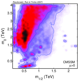
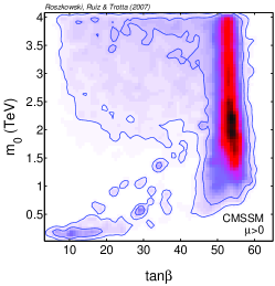
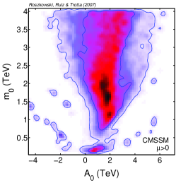
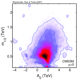
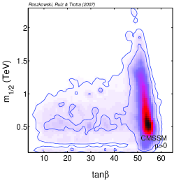
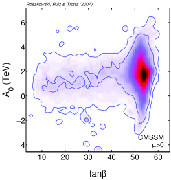
Figure 1: The 2-dim relative probability density functions in the planes spanned by the CMSSM parameters: $m_{1/2}$, $m_{0}$, $A_{0}$ and $\tan\beta$ for $\mu>0$. The pdf’s are normalized to unity at their peak. The inner (outer) blue solid contours delimit regions encompassing 68% and 95% of the total probability, respectively. All other basis parameters, both CMSSM and SM ones, in each plane have been marginalized over. This figure should be compared with figure 2 in ref. [14].

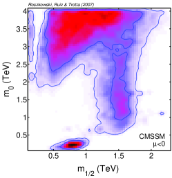
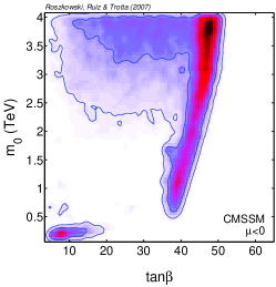
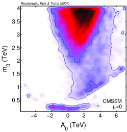
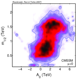
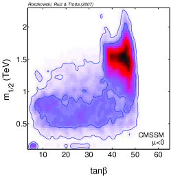
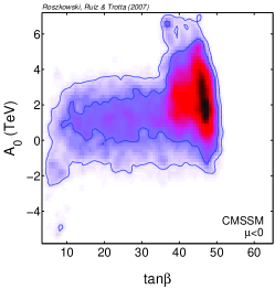
Figure 2: The same as in fig. 1 but for $\mu<0$.

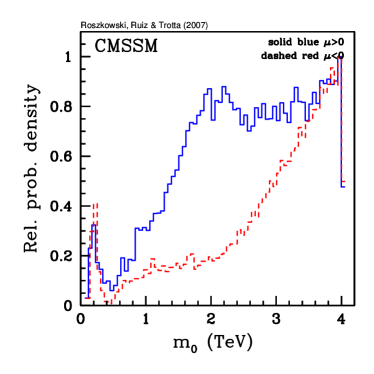
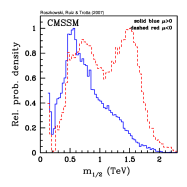
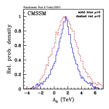
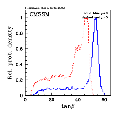
Figure 3: The 1-dim relative probability densities for the CMSSM parameters $m_{0}$, $m_{1/2}$, $A_{0}$ and $\tan\beta$. All other parameters have been marginalized over. Solid blue (dashed red) curves correspond to $\mu>0$ ($\mu<0$). This figure should be compared with figure 4 (black solid lines) in ref. [14].

We first show in fig. 1 the 2-dim relative probability density functions in the planes spanned by the CMSSM parameters: $m_{1/2}$, $m_{0}$, $\tan\beta$, $A_{0}$, and assuming $\mu>0$, while in fig. 2 the same is shown for $\mu<0$. In each panel all other basis parameters have been marginalized over. Redder (darker) regions correspond to higher probability density. Inner and outer blue (dark) solid contours delimit regions of 68% and 95% of the total probability, respectively, and remain well within the assumed priors, except for $m_{0}$. In all the 2-dim plots, the MC samples have been divided into $70\times 70$ bins, with a mild smoothing across adjacent bins to improve the quality of the presentation (this has not impact on our statistical conclusions). Jagged contours are a result of a finite resolution of the MC chains.

In the case of $\mu>0$ (fig. 1) we can see a strong preference for large $m_{0}\mathrel{\hbox to0.0pt{\lower 4.0pt\hbox{\hskip 1.0pt$\sim$}\hss}\raise 1.0pt\hbox{$>$}}1\mbox{ TeV}$. On the other hand, the peak of probability for $m_{1/2}$ is around $0.5\mbox{ TeV}$, although the 68% range of total probability is rather wide, increases with $m_{0}$ and exceeds $1.5\mbox{ TeV}$ for $m_{0}\simeq 4\mbox{ TeV}$. Additionally, at smaller $m_{0}\mathrel{\hbox to0.0pt{\lower 4.0pt\hbox{\hskip 1.0pt$\sim$}\hss}\raise 1.0pt\hbox{$<$}}1\mbox{ TeV}$ there are a few confined 68% total probability regions.

The strong preference for large $m_{0}\gg m_{1/2}$ is primarily the result of the sizable shift in the SM value of $BR(\overline{B}\rightarrow X_{s}\gamma)$, as can be seen by comparing fig. 1 with fig. 2 in ref. [14] (or fig. 8 of ref. [15]) where the previous value of $BR(\overline{B}\rightarrow X_{s}\gamma)$ has been used. (While the other CMSSM parameters also experience some shift in their most probable values, it is not as dramatic as that of $m_{0}$ towards larger values.) The underlying reason is that, at fairly small $m_{1/2}$ the charged Higgs mass remains relatively light, in the few hundred GeV range, and, via a loop exchange with the top quark, it adds substantially to the SM value of $BR(\overline{B}\rightarrow X_{s}\gamma)$, towards the experimentally allowed range. (In fact, for $m_{H^{-}}\simeq 650\mbox{ GeV}$, the contribution is sufficient to fill the gap between the SM and the experimental central values of $BR(\overline{B}\rightarrow X_{s}\gamma)$ [6].) At smaller $m_{1/2}$ and/or $m_{0}$, the (negative, for $\mu>0$) chargino-stop contribution is too large and needs to be compensated by the $H^{-}$-top contribution. In fact, we do find some small “islands” of 68% total probability at $m_{1/2}\mathrel{\hbox to0.0pt{\lower 4.0pt\hbox{\hskip 1.0pt$\sim$}\hss}\raise 1.0pt\hbox{$<$}}1\mbox{ TeV}$ and $m_{0}\mathrel{\hbox to0.0pt{\lower 4.0pt\hbox{\hskip 1.0pt$\sim$}\hss}\raise 1.0pt\hbox{$<$}}1.3\mbox{ TeV}$ (in particular, notably, an interesting case of $m_{1/2}\simeq 0.5\mbox{ TeV}$ and $m_{0}\simeq 0.2\mbox{ TeV}$) but the bulk of high probability region corresponds to $m_{0}\mathrel{\hbox to0.0pt{\lower 4.0pt\hbox{\hskip 1.0pt$\sim$}\hss}\raise 1.0pt\hbox{$>$}}1\mbox{ TeV}$.

At $95\%$ total probability level the available parameter space opens widens considerably, and also some new features arise. In particular, at $m_{1/2}\simeq 0.2\mbox{ TeV}$ we can see a narrow high-probability funnel induced by the light Higgs boson resonance [12, 14]. Also, $\tan\beta$ becomes less confined to its most preferred range of large values between some 50 and 60, while $A_{0}$ remains on a positive side.

In the case of $\mu<0$ (fig. 2), one can see a strong preference for even larger $m_{0}$. Also, the 68% total probability region of $m_{1/2}$ shifts towards larger values, although still remains basically below $2\mbox{ TeV}$. (Although we again find an interesting isolated high probability region at $m_{1/2}\simeq 0.75\mbox{ TeV}$ and $m_{0}\simeq 0.2\mbox{ TeV}$.) This shift towards larger $m_{0}$ and/or $m_{1/2}$ is again caused mostly by the $BR(\overline{B}\rightarrow X_{s}\gamma)$ constraint. At large $m_{0}$ (and not too large $m_{1/2}$) the charged Higgs mass decreases and its contribution tends to be on a high side, while the chargino-stop one becomes too small. A similar effect is observed at large $m_{1/2}\sim 1.5\mbox{ TeV}$ and $m_{0}\mathrel{\hbox to0.0pt{\lower 4.0pt\hbox{\hskip 1.0pt$\sim$}\hss}\raise 1.0pt\hbox{$>$}}1\mbox{ TeV}$ where the chargino and stop masses become too large to contribute much as well.

In fig. 3 the 1-dim marginalized probability distributions for the CMSSM parameters are compared for both $\mu>0$ and $\mu<0$. In each panel all the other CMSSM parameters and all SM (nuisance) parameters have been marginalized over. It is clear that non-negligible probability ranges of the CMSSM parameters, other than $m_{0}$, are confined well within their assumed priors. Again, we can see strong preference for large $m_{0}\gg 1\mbox{ TeV}$ (even stronger for $\mu<0$ than for $\mu>0$). Larger values of $m_{1/2}$ are also favored for $\mu<0$ although, for both signs, this parameter is well confined within $2\mbox{ TeV}$. The preferred range of $A_{0}$ is fairly uncorrelated with the other parameters [14], and it is symmetrically peaked (basically independently of the sign of $\mu$) at some $1.5\mbox{ TeV}$. This value is however basically twice as large as for the previous SM value of $BR(\overline{B}\rightarrow X_{s}\gamma)$ [14]. On the other hand, $\tan\beta$ is well-peaked at some $53$ for $\mu>0$ and some $48$ for $\mu<0$. In both cases, there remains a sizable tail of much smaller values which remain allowed at large $m_{0}$.

What most strongly contributes to confining $m_{1/2}$ well within its prior (for both signs of $\mu$) is the relic abundance $\Omega_{\chi}h^{2}$ which becomes too large. On the one hand, at large $\tan\beta$ it becomes easier to satisfy the constraint from $\Omega_{\chi}h^{2}$ due to the increased role of the neutralino annihilation via the pseudoscalar Higgs effect and/or the coannihilation effect. On the other, as explained in ref. [14, 16], as $\tan\beta$ becomes very large, $\mathrel{\hbox to0.0pt{\lower 4.0pt\hbox{\hskip 1.0pt$\sim$}\hss}\raise 1.0pt\hbox{$>$}}60$ for $\mu>0$ ($\mathrel{\hbox to0.0pt{\lower 4.0pt\hbox{\hskip 1.0pt$\sim$}\hss}\raise 1.0pt\hbox{$>$}}50$ for $\mu<0$), it becomes very difficult to find self-consistent solutions of the RGE’s.

The feature that very large values of $m_{0}$ (the FP region), up to the assumed prior of $4\mbox{ TeV}$, remain allowed (actually, even preferred), is unfortunate but is a consequence of the fact that current data are not constraining enough. Normally, as all the superpartner masses (including the LSP) increase, bino-like neutralino annihilation in the early Universe becomes suppressed and it becomes harder to satisfy the WMAP constraint on $\Omega_{\chi}h^{2}$. This is why $m_{1/2}$ is well confined within some $2\mbox{ TeV}$, as described above. Unfortunately, in the FP region the behavior of $\Omega_{\chi}h^{2}$ is much more sensitive to input parameters. We illustrate this in fig. 4 where we plot $\Omega_{\chi}h^{2}$ vs. $m_{0}$ for $\mu>0$ and a choice of the other CMSSM parameters close to their highest probability values (fig. 1). Clearly, as $M_{t}$ is varied within $1\sigma$ around its central value (cv), $\Omega_{\chi}h^{2}$ changes quite substantially. In the presented example, by fixing $M_{t}$ at its central value [36] (as it is normally done in fixed-grid scans) one would find no cosmologically allowed $m_{0}$. On the other hand, by reducing (increasing) $M_{t}$ by $1\sigma$ we can find one (two widely disconnected ) narrow region(s) of $m_{0}$ where $\Omega_{\chi}h^{2}$ in the WMAP range. Furthermore, in a probabilistic approach, even the case at the central value of $M_{t}$ is not excluded but only less favored by $\Omega_{\chi}h^{2}$.

Another feature that is evident in fig. 4 is that, as $M_{t}$ is varied by $1\sigma$ around its central value, the range of $m_{0}$ where self-consistent solutions of the RGE’s and the conditions of EWSB can be found changes by as much as a factor of two. It is therefore clear that, if one includes the FP region, it is basically impossible to locate the cosmologically favored range of $m_{0}$. In particular, it would be misleading to simply fix the top mass at its central value (and likewise with the bottom mass at large $\tan\beta$).

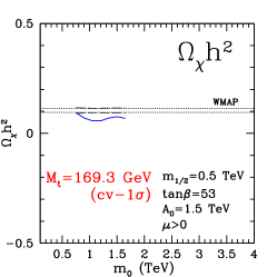
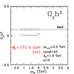
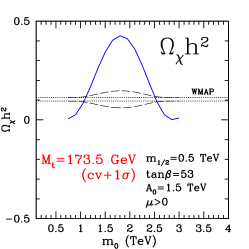
Figure 4: An illustration of the sensitivity of the cosmologically favored range of $m_{0}$ to the top mass $M_{t}$ in the focus point region. Other CMSSM parameters have been fixed close to their most preferred values for $\mu>0$ (see fig. 1). We show $\Omega_{\chi}h^{2}$ (blue solid line) for the central value (cv) of $M_{t}$ (middle panel) and for the values decreased and increased by $1\sigma$ (left and right panel). The parallel dotted lines denote the very narrow $2\sigma$ range, as determined from the 3-year data of WMAP [23]. The long-dashed line denotes the combined theoretical plus experimental error, as described in the text. Note that, as $M_{t}$ is varied between its cv minus $1\sigma$ to its cv plus $1\sigma$, the range of $m_{0}$, for which consistent solutions can be found, roughly doubles.

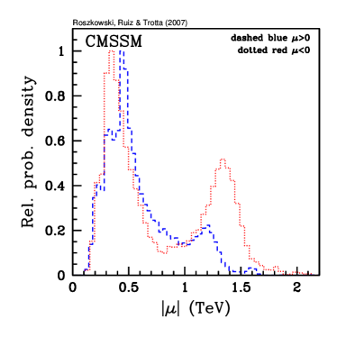
Figure 5: The 1-dim relative probability density of $|\mu|$. All other parameters have been marginalized over. Dashed blue (dotted red) curves correspond to $\mu>0$ ($\mu<0$).

The rather special properties of the FP region are to a large extent related to the behavior of the parameter $\mu$. As $m_{0}$ increases (along, say, fixed $m_{1/2}$), $\mu^{2}$ (which is determined the the conditions of EWSB) decreases rather quickly, thus increasing the higgsino component of the neutralino. This in turn reduces $\Omega_{\chi}h^{2}$ to an acceptable range for some narrow range of $m_{0}$. At slightly larger $m_{0}$, $\mu^{2}$ drops below zero, thus delimiting the zone where consistent, non-tachyonic solutions can be found. Thus generally in the FP region $\mu$ is rather small relative to $m_{0}$. We can see this feature in fig. 5 where we plot the 1-dim relative probability density for the parameter. We can see a clear peak in the few hundred GeV region for both signs of $\mu$. In this region $|\mu|\simeq m_{1/2}/3$. Additionally, for $\mu<0$ there is a second well-pronounced peak around some $1.4\mbox{ TeV}$ which corresponds to the band of higher relative probability around $m_{1/2}\simeq 1.5\mbox{ TeV}$ and $m_{0}\mathrel{\hbox to0.0pt{\lower 4.0pt\hbox{\hskip 1.0pt$\sim$}\hss}\raise 1.0pt\hbox{$>$}}1\mbox{ TeV}$ in fig. 2, outside of the FP region.

	$\mu<0$		$\mu>0$
Parameter	68% region	95% region	68% region	95% region
$m_{0}$ (TeV)	$<3.51$	$<3.93$	$<3.1$	$<3.87$
$m_{1/2}$ (TeV)	$(0.57,1.55)$	$(0.87,1.86)$	$(0.4,1.16)$	$(0.145,1.6)$
$A_{0}$ (TeV)	$(-0.19,3.42)$	$(-1.79,5.49)$	$(0.11,2.94)$	$(-1.86,4.84)$
$\tan\beta$	$(18.6,46.08)$	$(7.51,48.9)$	$(26.38,54.18)$	$(11.17,56.78)$

Table 3: CMSSM parameter ranges corresponding to 68% and 95% of posterior probability (with all other parameters marginalized over) for both signs of $\mu$.

In order to summarize the above discussion, in table 3 we give the 68% and 95% total probability ranges of the CMSSM parameters for both signs of $\mu$.

We emphasize that the above results do not at all imply that it is equally easy to fit all the data for both signs of $\mu$. (In figs. 1– 3 the posterior probabilities are normalized relative to the respective highest values.) Actually, for negative $\mu$ the fit is considerably poorer. In fact, we find that the best-fit $\chi^{2}$ for the $\mu>0$ case is $6.3$, while for the $\mu<0$ case it more than doubles to $14.4$. It is difficult to attach a precise statistical significance to this result, as clearly the distributional properties of the parameter space are far from being Gaussian (and hence the $\chi^{2}$ is not chi-square distributed). A proper evaluation of the significance of this difference in the goodness-of-fit would require Monte Carlo simulations of the measurements for both the $\mu>0$ and $\mu<0$ cases, which is beyond the scope of this work. However, this is an indication of the fact that the $\mu<0$ case is at greater tension with the data than $\mu>0$, although it cannot be conclusively ruled out yet.

A fully Bayesian approach would consider computing the Bayes factor among the two possibilities for $\mu$, along the lines of what has been done in ref. [15]. This procedure is, however, computationally demanding, and the result is potentially strongly dependent on volume effects deriving from the choice of priors (see, eg., ref. [37]). An interesting alternative is to use the procedure outlined in ref. [38] which employs Bayesian calibrated p-values to obtain an upper limit on the Bayes factor regardless of the prior for the alternative hypothesis. In the present case, the application of this procedure would require Monte Carlo simulation to obtain the p-value corresponding to the observed $\chi$-square difference. However, if we take again the result of $\Delta\chi^{2}=7$ at face value, assuming that it is indeed $\chi$-square distributed (which is probably a very poor approximation, as argued above), then the corresponding upper limit on the Bayes factor is $10:1$. (This rough estimate is actually in surprising good agreement with the result found in ref. [15] using numerical integrations) This would mean that the minimum probability of $\mu<0$ is 0.1, which certainly does not constitute strong evidence against $\mu<0$. The above considerations only highlight the difficulty of translating our result into a precise statement about the relative probability of $\mu>0$ vs $\mu<0$.

A related (although somewhat different) issue is to identify regions of the CMSSM PS where the fit to the data is much better than elsewhere. As stated above, if such regions occupy a small volume of parameter space (given our choice of priors), the posterior pdf will consequently weight them down, although they might exhibit a higher goodness-of-fit. To address this point, we consider an alternative measure of the mean quality-of-fit, which is defined as the average of the effective $\chi^{2}$ under the posterior distribution, i.e.,

$$\langle\chi^{2}\rangle=\int d\,m\,[-2\ln{p(d|m)}]p(m|d),$$ (5)

which is a quantity that is largely insensitive to the choice of priors (as long as the best-fitting points are explored by the MCMC scan). Its distribution for the CMSSM parameters is plotted in figs. 6 and 7 for $\mu>0$ and $\mu<0$, respectively, in each case they are normalized to the respective best-fit value. We can see that, for $\mu>0$, there indeed exists at least one well-localized region around $m_{1/2}\simeq 0.4\mbox{ TeV}$ and $m_{0}\simeq 1.5\mbox{ TeV}$ (not far from the location of the highest relative pdf, and in any case within the 68% total probability contour), with another one at somewhat smaller values of both $m_{1/2}$ and $m_{0}$. (Below we will show however that such best-fit regions may be in conflict with dark matter search limits, which have not been applied as constraints at this stage.) On the other hand, at $\mu<0$ it is generally more difficult to find a good fit to the data, as indicated by the larger value of the $\chi^{2}$ given above. We also notice that many of the best-fitting regions for the case $\mu<0$ in fig. 7 lie outside the $95\%$ posterior probability contour, further indicating a strong tension with the data.

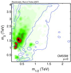
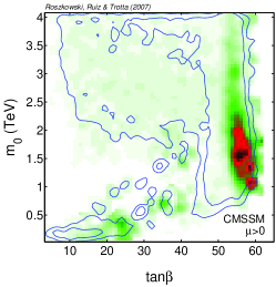
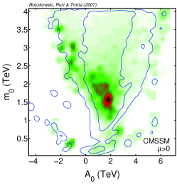
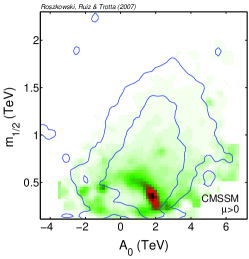
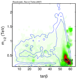
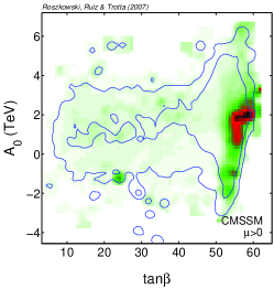
Figure 6: The mean quality-of-fit in the planes spanned by the CMSSM parameters: $m_{1/2}$, $m_{0}$, $A_{0}$ and $\tan\beta$ for $\mu>0$. For comparison, (blue solid) total posterior probability contours of 68% and 95% from fig. 1 have been added. This figure should be compared with figure 11 in ref. [14].

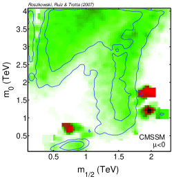
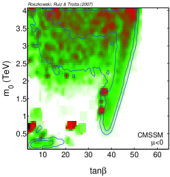
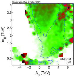
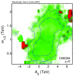
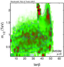
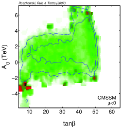
Figure 7: The same as in fig. 6 but for $\mu<0$. For comparison, (blue solid) total posterior probability contours of 68% and 95% from fig. 2 have been added.

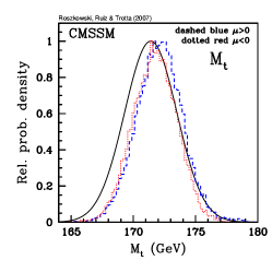
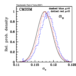
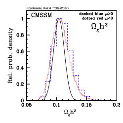
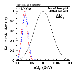
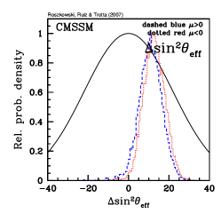
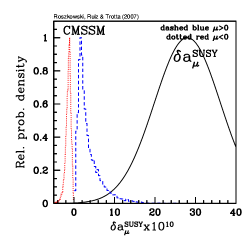
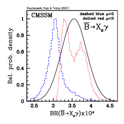
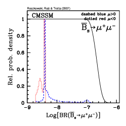
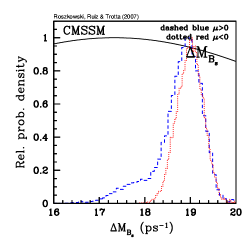
Figure 8: The 1-dim relative probability density functions for several variables: $M_{t}$, $\alpha_{s}(M_{Z})^{\overline{MS}}$, $\Omega_{\chi}h^{2}$, $\Delta m_{W}=m_{W}-80.392\mbox{ GeV}$, $\Delta\sin^{2}\theta_{\text{eff}}{}=\sin^{2}\theta_{\text{eff}}{}-0.23153$, $BR(\overline{B}\rightarrow X_{s}\gamma)$, $\delta a_{\mu}^{\text{SUSY}}$, $BR(\overline{B}_{s}\to\mu^{+}\mu^{-})$, $\Delta M_{B_{s}}$. In each panel the dashed blue (dotted red) curves correspond to $\mu>0$ ($\mu<0$) while the black solid line represents the data as encoded in the likelihood function. This figure should be compared with figure 10 in ref. [14].

Different experimental observables may constrain or favor different regions of the CMSSM parameters; they may “pull” in different directions. We display this in fig. 8 where we plot the 1-dim posterior pdf’s for several variables for both signs of $\mu$. For comparison, we also plot the corresponding Gaussian likelihood functions representing the data used in the fit. If there was no tension among different observables then, in the absence of strong correlations among them, the relative probability curves should overlap with the data. This is basically the case for $M_{t}$, $\alpha_{s}(M_{Z})^{\overline{MS}}$ and $\Omega_{\chi}h^{2}$. (In the last case the slightly skewed shape of the pdf’s is a result of our treatment of the theoretical uncertainty which is larger for larger $\Omega_{\chi}h^{2}$.) On the other hand, the electroweak observables $m_{W}$ and $\sin^{2}\theta_{\text{eff}}{}$ show some pull away from their expected values, in general agreement with ref. [15] where the two variables were computed with a similar precision. On the other hand, the tension is insufficient to provide convincing preference for low $M_{\rm SUSY}$, in apparent contrast to the findings of ref. [36].

The biggest tension between best-fit values and experiment is displayed, unsurprisingly, in the SUSY contribution to the anomalous magnetic moment of the muon. For both signs of $\mu$ the peaks of the relative probability are far below the central experimental value (about $3.2\sigma$ for $\mu>0$ versus about $3.7\sigma$ for $\mu<0$), and close to each other [15]. We conclude that it is not justified to use this sole observable to select the positive sign of $\mu$ – one has to perform a global fit in all of the variables and judge the two cases by this criterion. Furthermore, the new $BR(\overline{B}\rightarrow X_{s}\gamma)$ actually seems to agree with the data slightly better for $\mu<0$ than for the other sign. Generally, for $\mu>0$ the total $BR(\overline{B}\rightarrow X_{s}\gamma)$ remains peaked around the SM central value, while for $\mu<0$ it is somewhat above it. Finally, $BR(\overline{B}_{s}\to\mu^{+}\mu^{-})$ and $\Delta M_{B_{s}}$ are peaked at their SM values, somewhat more so than before [14].

3.2 Implications for collider searches

In our Bayesian formalisms, high probability ranges of the CMSSM parameters can easily be translated into analogous ranges for Higgs and superpartner masses, and for other observables, including indirect processes and dark matter detection cross sections. We discuss them in turn below.

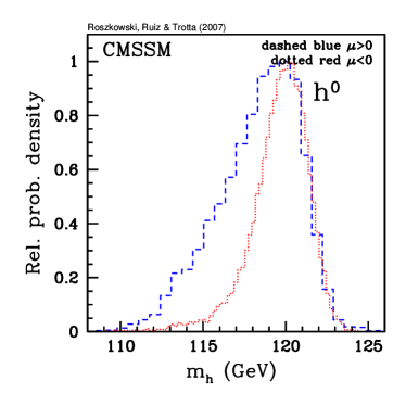
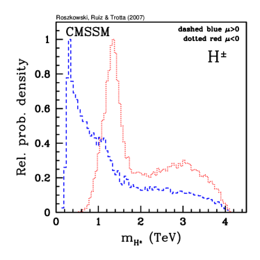
Figure 9: The 1-dim relative probability density functions for the masses of $h^{0}$ (left panel) and $H^{\pm}$ (right panel). Dashed blue (dotted red) curves correspond to $\mu>0$ ($\mu<0$). Analogous and more detailed figures for the case $\mu>0$ were presented in fig. 7 of ref. [16].

We start with the Higgs bosons. In fig. 9 we plot the Bayesian relative probability density distributions of the mass of the lightest Higgs boson $h^{0}$ and of the charged Higgs boson $H^{\pm}$ for both signs of $\mu$. (The other Higgs bosons are basically degenerate in mass with $H^{\pm}$.) In both cases we can see a clear peak in $m_{h}$ close to $120\mbox{ GeV}$, and a sharp drop-off for larger values of the mass. The other Higgs are typically considerably heavier for negative $\mu$ than for the other choice. This may provide one way of an experimental determination of the sign of $\mu$. The 68% and 95% total probability ranges of the Higgs masses are given in table 4 below. We should also note that the alternative measure of the mean quality-of-fit favors lower ranges of the masses of all the Higgs bosons in the case of $\mu>0$ [16]. For the case $\mu<0$, the mean quality-of-fit distribution of $m_{h}$ is roughly similar to that of the pdf but with the peak shifted to the right by about $1\mbox{ GeV}$ (plus some moderate preference for smaller values, around the current LEP-II limit), while the masses of all the other Higgs bosons are preferably very heavy, in the TeV regime. This is a reflection of the absence of regions giving good fit to the data in the case of $\mu<0$ (compare fig. 7).

In ref. [16] we have investigated in detail light Higgs masses and couplings for the case of $\mu>0$. In particular we showed that, throughout the whole CMSSM parameter space, the couplings of the lightest Higgs boson $h^{0}$ to the gauge bosons $Z$ and $W$ are very close to those of the SM Higgs boson with the same mass, while its couplings to bottom quark and tau lepton pairs show some variation. We concluded that, at the Tevatron, with about $2\,\mbox{fb}^{-1}$ of integrated luminosity per experiment (already on tape), it should be possible to set a 95% CL exclusion limit for the whole 95% posterior probability range of $m_{h}$. Based on fig. 9 and table 4 we extend this conclusion to the case of $\mu<0$. On the optimistic side, should a Higgs signal be found, in order to be able to claim a $3\sigma$ evidence, at least about $4\,\mbox{fb}^{-1}$ will be needed, independently of the sign of $\mu$. The Tevatron’s ultimate goal is to collect about $8\,\mbox{fb}^{-1}$ per experiment.

One should remember that the above conclusions do depend on the assumed prior range of $m_{0}<4\mbox{ TeV}$, as well as on the choice of adopting flat priors in the CMSSM variables of eq. 1. For instance, adopting a much more generous upper limit $m_{0}<8\mbox{ TeV}$ would lead to changing the ranges for $\mu>0$ to roughly $120.4\mbox{ GeV}\mathrel{\hbox to0.0pt{\lower 4.0pt\hbox{\hskip 1.0pt$\sim$}\hss}\raise 1.0pt\hbox{$<$}}m_{h}\mathrel{\hbox to0.0pt{\lower 4.0pt\hbox{\hskip 1.0pt$\sim$}\hss}\raise 1.0pt\hbox{$<$}}124.4\mbox{ GeV}$ (68% CL) and $115.4\mbox{ GeV}\mathrel{\hbox to0.0pt{\lower 4.0pt\hbox{\hskip 1.0pt$\sim$}\hss}\raise 1.0pt\hbox{$<$}}m_{h}\mathrel{\hbox to0.0pt{\lower 4.0pt\hbox{\hskip 1.0pt$\sim$}\hss}\raise 1.0pt\hbox{$<$}}125.6\mbox{ GeV}$ (95% CL), the latter of which could be excluded at 95% CL with about $3\,\mbox{fb}^{-1}$ of integrated luminosity per experiment [16]. Still, should no Higgs signal be found at the Tevatron, large ranges of $m_{0}$ will become excluded at high CL, with the specific value depending on the accumulated luminosity.

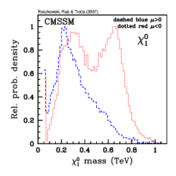
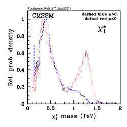
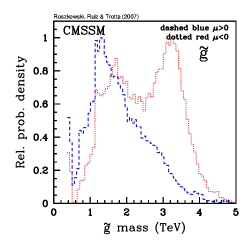
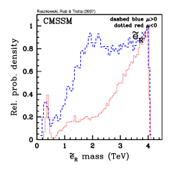
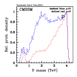
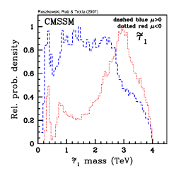
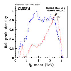
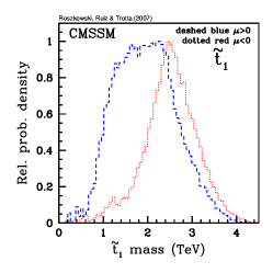
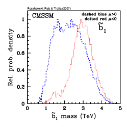
Figure 10: As in fig. 3, but for the masses of several representative superpartners. This figure should be compared with figure 5 (black solid lines) in ref. [14].

Turning next to superpartners, we show in fig. 10 the relative pdf’s of the masses of several of them, while in table 4 we give the corresponding 68% CL and 95% CL ranges. The blue dashed curves are for $\mu>0$ and the red dotted ones for $\mu<0$. Firstly, for $\mu<0$ all the scalar superpartners are considerably heavier than for the other sign of $\mu$, as expected based on the discussion of most probable ranges of $m_{1/2}$ and especially $m_{0}$. In fact, if $\mu<0$ then all the sleptons and squarks (whose masses, except for the 3rd generation, are at least as large as $m_{0}$) may be beyond the reach of the LHC. For $\mu>0$ there is a good chance of seeing the gluino (assuming the LHC reach of some $2.7-3\mbox{ TeV}$) and a reasonable chance of seeing some squarks and sleptons. Unfortunately, these prospects are considerably less optimistic than what we found in fig. 5 and table 6 of ref. [14], where the previous SM value of $BR(\overline{B}\rightarrow X_{s}\gamma)$ was used. A dedicated analysis would be required to derive more detailed conclusions.

Particle	$\mu<0$		$\mu>0$
(TeV)	68%	95%	68%	95%
$h^{0}$	$(0.1180,0.1211)$	$(0.1151,0.1223)$	$(0.1154,0.1204)$	$(0.1125,0.1219)$
$H^{0},A^{0},H^{\pm}$	$(1.2,3.1)$	$(0.91,3.8)$	$(0.36,2.5)$	$(0.21,3.6)$
$\chi_{1}^{0}$	$(0.23,0.67)$	$(0.11,0.82)$	$(0.16,0.49)$	$(0.06,0.69)$
$\chi_{1}^{\pm}$	$(0.3,1.2)$	$(0.15,1.4)$	$(0.25,0.76)$	$(0.11,1.2)$
$\widetilde{g}$	$(1.4,3.4)$	$(0.77,4.0)$	$(1.0,2.6)$	$(0.41,3.5)$
$\tilde{e}_{R}$	$(1.8,3.8)$	$(0.37,4.0)$	$(1.5,3.6)$	$(0.5,4.0)$
$\tilde{\nu}$	$(1.9,3.8)$	$(0.58,4.0)$	$(1.6,3.6)$	$(0.65,4.0)$
$\tilde{\tau}_{1}$	$(1.4,3.3)$	$(0.34,3.8)$	$(0.80,2.8)$	$(0.28,3.7)$
$\tilde{q}_{R}$	$(2.9,4.3)$	$(1.6,4.9)$	$(1.9,4.0)$	$(1.3,4.7)$
$\tilde{t}_{1}$	$(1.9,3.1)$	$(1.1,3.6)$	$(1.3,2.6)$	$(0.86,3.3)$
$\tilde{b}_{1}$	$(2.3,3.5)$	$(1.4,4.1)$	$(1.4,3.1)$	$(1.0,3.8)$

Table 4: Higgs boson and selected superpartner mass ranges (in TeV) containing 68% and 95% of posterior probability (with all other parameters marginalized over) for both signs of $\mu$. Masses above $1\mbox{ TeV}$ have been rounded up to 1 significant digit.

3.3 Implications for direct detection of Dark Matter

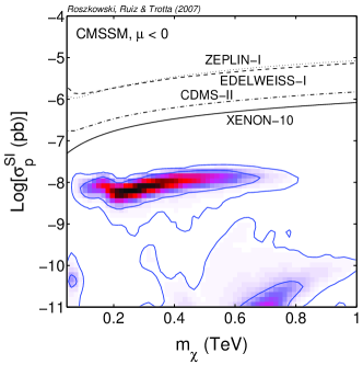
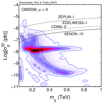
Figure 11: The 2-dim relative probability density for $\sigma^{SI}_{p}$ vs. the neutralino mass $m_{\chi}$ for $\mu<0$ (left panel) and $\mu>0$ (right panel). The inner (outer) solid contours delimit the regions of 68% and 95% total probability, respectively. Some current experimental upper bounds are also shown. The right panel should be compared with figure 13 (top) in ref. [14].

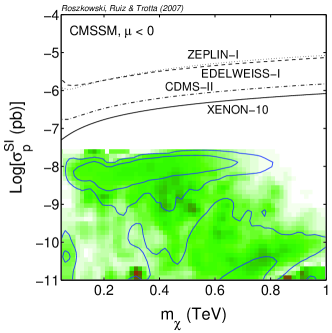
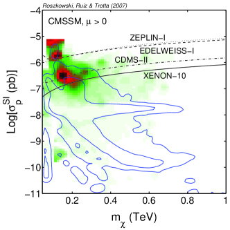
Figure 12: The mean quality-of-fit for $\sigma^{SI}_{p}$ vs. the neutralino mass $m_{\chi}$ for $\mu<0$ (left panel) and $\mu>0$ (right panel). The inner (outer) solid contours delimit the regions of posterior 68% and 95% total probability, respectively (compare fig. 11). Some current experimental upper bounds are also shown, but have not been included as constraints in the likelihood function. The right panel should be compared with figure 13 (bottom) in ref. [14].

We will now examine implications for direct detection of the lightest neutralino assumed to be the DM in the Universe, via its elastic scatterings with targets in underground detectors [4]. We will consider both spin-independent (SI) and spin-dependent (SD) interactions. The underlying formalism for both types of interactions can be found in several sources. (See, e.g., [39, 4, 40, 41].) In this analysis we use the expressions and inputs as presented in ref. [41]. We only note here that the SI interactions cross section $\sigma^{SI}_{p}$ of a WIMP scattering off a proton in a target nucleus is the same as that of a neutron and that the total SI interactions cross section of the nucleus is proportional to $\sigma^{SI}_{p}$ times the square of the mass number. In contrast, for the SD interactions, the cross section for a WIMP scattering off a proton, $\sigma^{SD}_{p}$, does not necessarily have to be the same as the one from a neutron [42, 43].

In fig. 11 we show the Bayesian posterior relative probability distribution in the usual plane of $\sigma^{SI}_{p}$ and the DM neutralino mass $m_{\chi}$ for $\mu<0$ (left panel) and $\mu>0$ (right panel). Starting with $\mu>0$, we can see a big concentration of probability density at rather high values of $\sigma^{SI}_{p}\sim 10^{-8}\,\mbox{pb}$, characteristic of the FP region of large $m_{0}$ [44], which is favored by the current theoretical evaluation of $BR(\overline{B}\rightarrow X_{s}\gamma)$, as we have seen above. In the FP region, the neutralino, while remaining predominantly bino-like, receives a sizable higgsino component, which strengthens the dominant Higgs-exchange contribution to $\sigma^{SI}_{p}$. In addition, there is a more well-known branch, with $\sigma^{SI}_{p}$ decreasing with $m_{\chi}$, which comes from the (now somewhat disfavored) region of $m_{1/2},m_{0}\mathrel{\hbox to0.0pt{\lower 4.0pt\hbox{\hskip 1.0pt$\sim$}\hss}\raise 1.0pt\hbox{$<$}}1\mbox{ TeV}$ where the relic abundance $\Omega_{\chi}h^{2}$ of the neutralinos is reduced to agree with WMAP and other determinations by a pseudoscalar Higgs resonance in their pair annihilation and/or by their coannihilations with sleptons. In order to appreciate the change in the CMSSM predictions for $\sigma^{SI}_{p}$, the right panel should be compared with the top panel of fig. 13 in ref. [14] where a previous value of the SM prediction for $BR(\overline{B}\rightarrow X_{s}\gamma)$ was used.

The left panel of fig. 11 (the case of $\mu<0$) also shows a high preference for $\sigma^{SI}_{p}\sim 10^{-8}\,\mbox{pb}$, which corresponds to the FP region at multi-TeV $m_{0}$, as for the other sign of $\mu$. In addition, we find another rather large 68% total probability region at extremely low values of below $10^{-10}\,\mbox{pb}$, which corresponds to the higher probability region of $m_{1/2}\sim 1.5\mbox{ TeV}$ in the $(m_{1/2},m_{0})$ plane. Such tiny ranges of $\sigma^{SI}_{p}$ are a result of cancellation between the Higgs-exchange contribution to up- and down-type quarks [39, 40].

In both panels of fig. 11 we have marked some of the current direct experimental upper limits [45, 46, 47], assuming a default value of $0.3\mbox{ GeV}/{\rm cm}^{3}$ for the local DM density. It is encouraging that experiments, notably XENON-10 with its very new limit, are already probing some portions of the CMSSM PS for $\mu>0$. CDMS-II is currently taking data and is expecting to improve its limit to a similar level of sensitivity. Clearly, a further improvement by about an order of magnitude will constitute a critical leap as it will hopefully allow one to reach down to the heart of the SI interactions cross sections favored in the CMSSM. Future one-tonne detectors are expected to reach down to $\sigma^{SI}_{p}\mathrel{\hbox to0.0pt{\lower 4.0pt\hbox{\hskip 1.0pt$\sim$}\hss}\raise 1.0pt\hbox{$>$}}10^{-10}\,\mbox{pb}$, thus probing most of the favored parameter space of the CMSSM, at least for the more favored case of $\mu>0$. We note that the probability of $\sigma^{SI}_{p}>10^{-10}\,\mbox{pb}$ in fig. 11 is $98.4\%$ for $\mu>0$ and $62.5\%$ for $\mu<0$.

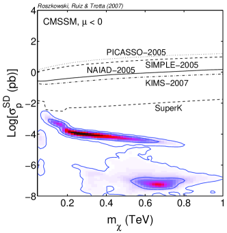
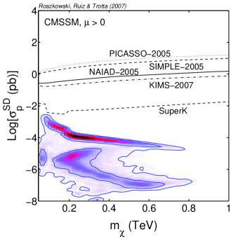
Figure 13: The 2-dim relative probability density of $\sigma^{SD}_{p}$ vs. the neutralino mass $m_{\chi}$ for $\mu<0$ (left panel) and $\mu>0$ (right panel). The inner (outer) solid contours delimit the regions of 68% and 95% total probability, respectively. Some current experimental 90% CL upper bounds are also shown. Analogous plots for $\sigma^{SD}_{n}$ are basically identical but the experimental limits from direct detection are weaker by nearly two orders of magnitude.

It is worth re-emphasizing that, in addition to light Higgs searches at the Tevatron and the LHC, direct detection DM searches will provide an alternative experimental probe of the FP region at multi-TeV $m_{0}$, in which the squarks will be too heavy to be produced at the LHC, although the gluino mass should remain mostly (partly) accessible for $\mu>0$ ($\mu<0$).

For comparison, fig. 12 shows the ranges favored by the alternative measure of the mean quality-of-fit. Starting with the case of $\mu>0$ (the right panel), we can see a handful of small regions of a rather large $\sigma^{SI}_{p}$, above a few times $10^{-7}\,\mbox{pb}$, which are already in conflict with the current limit from the XENON-10. These cases corresponds to the “islands” of good fit to the data that we have already seen in fig. 6, where they are all concentrated in the region of $m_{1/2}\mathrel{\hbox to0.0pt{\lower 4.0pt\hbox{\hskip 1.0pt$\sim$}\hss}\raise 1.0pt\hbox{$<$}}0.5\mbox{ TeV}$ and $m_{0}\mathrel{\hbox to0.0pt{\lower 4.0pt\hbox{\hskip 1.0pt$\sim$}\hss}\raise 1.0pt\hbox{$<$}}1.5\mbox{ TeV}$. With a modest improvement of sensitivity, DM search experiments will be able to probe the entire region favored by the mean quality-of-fit in the case of $\mu>0$. (Notice that neither the posterior pdf nor the mean quality-of-fit give much preference for very small $\sigma^{SI}_{p}$.) In contrast, for $\mu<0$ (the left panel of fig. 12) there is hardly any region giving good quality fits. This is a reflection of what we have already seen in the $(m_{1/2},m_{0})$ plane in fig. 7.

Turning next to SD interactions, in fig. 13 we present the relative probability density for neutralino-proton scattering cross section $\sigma^{SD}_{p}$ versus $m_{\chi}$ for $\mu<0$ (left panel) and $\mu>0$ (right panel). In the FP region the increased higgsino component of the neutralino in this case leads to a larger coupling to the dominant $Z$-boson exchange. This is reflected in the figure where the highest probability regions are, for both signs of $\mu$, concentrated around $\sigma^{SD}_{p}\sim 10^{-4}\,\mbox{pb}$. For $\mu>0$ there is an additional higher probability region which is visible in the right panel, and which corresponds to the Higgs resonance and coannihilation region mentioned above. In the case of $\mu<0$ instead, an additional higher probability region is visible in the left panel at $\sigma^{SD}_{p}\mathrel{\hbox to0.0pt{\lower 4.0pt\hbox{\hskip 1.0pt$\sim$}\hss}\raise 1.0pt\hbox{$<$}}10^{-7}\,\mbox{pb}$ and $m_{\chi}\sim 0.7\mbox{ TeV}$. It corresponds to the region of $m_{1/2}\sim 1.5\mbox{ TeV}$ in the $(m_{1/2},m_{0})$ plane (fig. 2).

The current experimental upper limits [48, 49, 50, 51] from direct searches, assuming a default value of $0.3\mbox{ GeV}/{\rm cm}^{3}$ for the local DM density, as well as an indirect limit from neutralino annihilations into neutrinos in the Sun, the Earth or the Galactic center [52], which have also been shown in fig. 13, still remain a few order of magnitude above the predictions of the CMSSM. On the other hand, experimental sensitivity has undergone steady progress also in the case of SD interactions. Eventually, it will be important to reach down below the level of $\sigma^{SD}_{p}\mathrel{\hbox to0.0pt{\lower 4.0pt\hbox{\hskip 1.0pt$\sim$}\hss}\raise 1.0pt\hbox{$<$}}10^{-4}\,\mbox{pb}$, which would allow one for an independent cross-check of CMSSM predictions for dark matter.

In table 5 we have listed the ranges of both $\sigma^{SI}_{p}$ and $\sigma^{SD}_{p}$ containing 68% and 95% of posterior probability (with all other parameters marginalized over) for both signs of $\mu$. The ranges cover the whole allowed range of $m_{\chi}$ and provide supplementary information to what one can read out of figs. 11 and 13.

	Spin-independent cross section $\sigma^{SI}_{p}$ ( pb)
	68%	95%
$\mu<0$	$(2.9\times 10^{-12},8.1\times 10^{-9})$	$(1.6\times 10^{-13},1.4\times 10^{-8})$
$\mu>0$	$(2.8\times 10^{-10},3.9\times 10^{-8})$	$(7.2\times 10^{-11},2.5\times 10^{-7})$
	Spin-dependent cross section $\sigma^{SD}_{p}$ ( pb)
	68%	95%
$\mu<0$	$(5.3\times 10^{-8},9.6\times 10^{-5})$	$(1.7\times 10^{-8},4.4\times 10^{-4})$
$\mu>0$	$(2.0\times 10^{-7},8.9\times 10^{-5})$	$(4.2\times 10^{-8},4.9\times 10^{-4})$

Table 5: Direct detection of dark matter: ranges of spin-independent and spin-dependent cross section corresponding to 68% and 95% of posterior probability (with all other parameters marginalized over) for both signs of $\mu$.

As mentioned above, in the SD interaction case the cross section of WIMP scattering from a neutron can in general be very different from the one from a proton. However, in our scan of the CMSSM, we have found its relatively probability distribution versus $m_{\chi}$ to be very close to the case with the proton, and thus do not show it here. As regards the mean quality-of-fit (not shown for $\sigma^{SD}_{p}$), at $\mu>0$ the best-fit regions in fig. 6 give a rather small value of $\sim 10^{-5}\,\mbox{pb}$, while at $\mu<0$ no range of $\sigma^{SD}_{p}$ is favored by the mean quality-of-fit criterion.

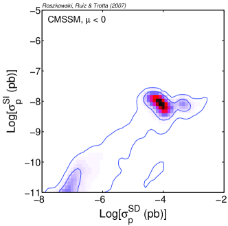
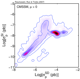
Figure 14: The 2-dim relative probability density of $\sigma^{SI}_{p}$ vs. $\sigma^{SI}_{p}$ for $\mu<0$ (left panel) and $\mu>0$ (right panel). The inner (outer) solid contours delimit the regions of 68% and 95% total probability, respectively. All other parameters have been marginalized over.

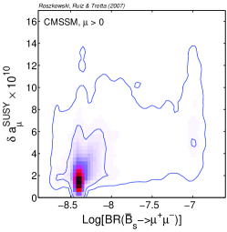
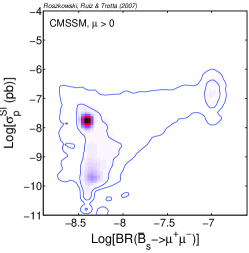
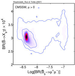
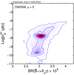
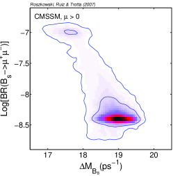
Figure 15: The 2-dim relative probability density for pairs of selected variables for $\mu>0$. The inner (outer) solid contours delimit the regions of 68% and 95% total probability, respectively. All other parameters have been marginalized over. This figure should be compared with figure 14 in ref. [14].

3.4 Correlations among observables

The probabilistic approach employed in this analysis makes it very easy to examine various possible global correlations among different observables in the CMSSM. For example, in fig. 14 we present the 2-dim pdf of $\sigma^{SI}_{p}$ versus $\sigma^{SD}_{p}$ for $\mu<0$ (left panel) and $\mu>0$ (right panel). For both signs of $\mu$ we can see a big concentration of probability density on $\sigma^{SI}_{p}\sim 10^{-8}\,\mbox{pb}$ and $\sigma^{SI}_{p}\sim 10^{-4}\,\mbox{pb}$, which is a reflection of their behavior in fig. 11) and fig. 13, respectively – an effect of the FP region. For $\mu>0$ we can see an additional feature of a positive correlation which is due to the contribution from the Higgs resonance and/or coannihilation effects.

More correlations are displayed in fig. 15 for the case of $\mu>0$. Again, the effect of the FP region is overwhelming. In all the observables, other than the dark matter SI cross section, SUSY effects likely to be tiny – the probability density is clearly peaked at the respective SM values. For $\mu<0$ (not displayed) the concentration is typically even stronger. Fig. 15 should be compared with fig. 14 of ref. [14] in order to appreciate the change. Some correlations which were quite well pronounced in that figure (eg. in $\sigma^{SI}_{p}$ versus $BR(\overline{B}_{s}\to\mu^{+}\mu^{-})$) are now barely visible.

4 Summary and conclusions

We have applied the highly efficient MCMC scanning method to explore the parameter space of the CMSSM and outlined the regions favored by the Bayesian posterior probability and, for comparison, by the mean mean quality-of-fit. We assumed flat priors in the usual CMSSM parameters, applied and updated all relevant experimental constraints from colliders and cosmological dark matter abundance, while paying particular attention to the impact of the recent change in the SM value of $BR(\overline{B}\rightarrow X_{s}\gamma)$. We examined both signs of $\mu$. For both choices, we found strong preference for the focus point region with large $m_{0}$ in the few TeV range (for $\mu<0$ actually saturating at the assumed prior boundary of $4\mbox{ TeV}$), and not as large $m_{1/2}\mathrel{\hbox to0.0pt{\lower 4.0pt\hbox{\hskip 1.0pt$\sim$}\hss}\raise 1.0pt\hbox{$<$}}2\mbox{ TeV}$. For comparison, the mean quality-of-fit measure selected a small number of isolated regions giving good fit to the data for $\mu>0$ but not for $\mu<0$. It appears that the choice $\mu<0$ is more at odds with the data, as reflected by its worse quality-of-fit.

We then examined ensuing implications for Higgs and superpartner searches and for direct detection of dark matter. Prospects for the Tevatron of excluding the whole 95% CL range of $m_{h}$ remain very good, or else there is very good hope to see at least some evidence of a signal with the expected final integrated luminosity. Scalar superpartner masses are typically heavier than $1\mbox{ TeV}$ (compare table 4) but there is a reasonable chance for at least some squarks (but probably no sleptons) to be seen at the LHC. On the other hand, the gluino, while also preferably heavy, should have a much better chance of discovery at the LHC. Prospects for detection are also promising in direct detection searches for dark matter which are sensitive to spin-independent interactions. An improvement in sensitivity down to $\sigma^{SI}_{p}\sim 10^{-8}\,\mbox{pb}$ will allow CDMS-II and other experiments to reach down to the bulk of the values favored by the posterior pdf (for both signs of $\mu$), and actually to fully explore all best-fit regions in the preferred case of $\mu>0$. On the other hand, an improvement in sensitivity of at least 3 orders of magnitude will be required before favored ranges of cross sections for spin-dependent neutralino-proton interactions are tested by experiment.

We stress that some of our findings do depend on our choice of the (usual) variables $m_{0}$, $m_{1/2}$, $A_{0}$ and, especially, $\tan\beta$ as CMSSM parameters over which we scan, and on the choice of taking flat priors on those variables. Of particular relevance is the upper bound $m_{0}<4\mbox{ TeV}$. Other choices are possible and should be examined. (See refs. [13, 53] and Note Added below.) The choice of CMSSM parameters and flat priors that we have made in the present analysis and the comparison with the mean-quality-of-fit statistics are meant to facilitate comparison with fixed-grid studies using similar assumptions.

Note added: Very recently, after our analysis was completed, a new paper of Allanach et al., [53] has appeared. The authors argue that, instead of assuming a flat prior in $\tan\beta$, it is more natural to use a “REWSB prior” where $\mu$ and the bi-linear soft mass parameter $B$ are taken as inputs with flat distributions. Whether this choice (originally advocated by R. Ratazzi) is superior to any other is debatable but it is certainly justifiable to apply it, at least for the sake of examining the sensitivity of observables to the choice of priors. We note that with the REWSB prior the preference for large $m_{0}$, well above $1\mbox{ TeV}$, still remains. (A more detailed comparison is difficult because in ref. [53] a previous SM value of $BR(\overline{B}\rightarrow X_{s}\gamma)$ has been used.) On the other hand, the authors in addition choose to give strong preference to cases where all the CMSSM mass parameters are of the same order. In our opinion this assumption does reflect a certain level of theoretical bias which at the end strongly changes the conclusions obtained with the REWSB prior only. (In particular it disfavors the focus point region which, as we have shown, can be seen as being favored by the current results on $BR(\overline{B}\rightarrow X_{s}\gamma)$.) We would prefer to see the lack of the hierarchy of the CMSSM mass parameters to be an outcome of applying experimental constraints, rather than of applying theoretical prejudice.

Acknowledgements
We are indebted to M. Misiak for providing to us a part of his code computing the SM value of $BR(\overline{B}\rightarrow X_{s}\gamma)$ and for several clarifying comments about the details of the calculation. L.R is partially supported by the EC 6th Framework Programmes MRTN-CT-2004-503369 and MRTN-CT-2006-035505. R.RdA is supported by the program “Juan de la Cierva” of the Ministerio de Educación y Ciencia of Spain. RT is supported by the Lockyer Fellowship of the Royal Astronomical Society and by St Anne’s College, Oxford. The author(s) would like to thank the European Network of Theoretical Astroparticle Physics ENTApP ILIAS/N6 under contract number RII3-CT-2004-506222 for financial support. This project benefited from the CERN-ENTApP joint visitor’s programme on dark matter, 5-9 March 2007.

References

-
[1]
See, e.g., H. E. Haber and G. L. Kane,
The Search for Supersymmetry: Probing Physics Beyond the Standard Model
Phys. Rept. 117 (1985) 75;
S. P. Martin, A Supersymmetry Primer, hep-ph/9709356. - [2] G. L. Kane, C. F. Kolda, L. Roszkowski and J. D. Wells, Study of constrained minimal supersymmetry, Phys. Rev. D 49 (1994) 6173 [hep-ph/9312272].
-
[3]
See, e.g., H. P. Nilles,
Supersymmetry, Supergravity and Particle Physics,
Phys. Rept. 110 (1984) 1;
A. Brignole, L. E. Ibañez and C. Muñoz, Soft supersymmetry breaking terms from supergravity and superstring models, published in Perspectives on Supersymmetry, ed. G. L. Kane, 125 [hep-ph/9707209]. -
[4]
See, e.g., G. Jungman, M. Kamionkowski
and K. Griest, Supersymmetric dark matter, Phys. Rept. 267 (1996) 195;
C. Muñoz, Dark Matter Detection in the Light of Recent Experimental Results, Int. J. Mod. Phys. A 19 (2004) 3093 [hep-ph/0309346]. - [5] Heavy Flavor Averaging Group (HFAG) (E. Barberio et al.), Averages of b-hadron properties at the end of 2005, hep-ex/0603003; for a very recent update see Heavy Flavor Averaging Group (HFAG) (E. Barberio et al.), Averages of b-hadron properties at the end of 2006, arXiv:0704.3575.
- [6] M. Misiak and M. Steinhauser, NNLO QCD corrections to the matrix elements using interpolation in , Nucl. Phys. B 764 (2007) 62 [hep-ph/0609241].
- [7] M. Misiak et al., Estimate of at , Phys. Rev. Lett. 98 (2007) 022002, [hep-ph/0609232].
- [8] T. Becher and M. Neubert, Analysis of at NNLO with a Cut on Photon Energy, Phys. Rev. Lett. 98 (2007) 022003 [hep-ph/0610067].
- [9] W.-M. Yao et al. [Particle Data Group], J. Phys. G33 (2006) 1.
- [10] See, e.g., B. A. Berg, Markov chain monte carlo simulations and their statistical analysis, World Scientific, Singapore (2004).
- [11] E. A. Baltz and P. Gondolo, Markov chain monte carlo exploration of minimal supergravity with implications for dark matter, J. High Energy Phys. 0410 (2004) 052 [hep-ph/0407039].
- [12] B. C. Allanach and C. G. Lester, Multi-dimensional MSUGRA likelihood maps, Phys. Rev. D 73 (2006) 015013 [hep-ph/0507283].
- [13] B. C. Allanach, Naturalness priors and fits to the constrained minimal supersymmetric standard model, Phys. Lett. B 635 (2006) 123 [hep-ph/0601089].
- [14] R. Ruiz de Austri, R. Trotta and L. Roszkowski, A Markov Chain Monte Carlo analysis of the CMSSM, J. High Energy Phys. 0605 (2006) 002 [hep-ph/0602028]; see also R. Trotta, R. Ruiz de Austri and L. Roszkowski, Prospects for direct dark matter detection in the Constrained MSSM, astro-ph/0609126.
- [15] B. C. Allanach, C. G. Lester and A. M. Weber, The dark side of mSUGRA, J. High Energy Phys. 0612 (2006) 065 [hep-ph/0609295].
- [16] L. Roszkowski, R. Ruiz de Austri and R. Trotta, On the detectability of the CMSSM light Higgs boson at the Tevatron, J. High Energy Phys. 0704 (2007) 084 [hep-ph/0611173].
- [17] R. Trotta, R. R. de Austri and L. Roszkowski, New Astron. Rev. 51 (2007) 316 [arXiv:astro-ph/0609126].
- [18] J. L. Feng, K. T. Matchev and T. Moroi, Multi - TeV scalars are natural in minimal supergravity, Phys. Rev. Lett. 84 (2000) 2322 [hep-ph/9908309] and Focus points and naturalness in supersymmetry, Phys. Rev. D 61 (2000) 075005 [hep-ph/9909334].
- [19] The Tevatron Electroweak Working Group, Combination of CDF and D0 results on the mass of the top quark, hep-ex/0608032.
- [20] Tevatron Electroweak Working Group (for the CDF and D0 Collaborations), A Combination of CDF and D0 Results on the Mass of the Top Quark, hep-ex/0703034.
- [21] See http://lepewwg.web.cern.ch/LEPEWWG.
- [22] The CDF Collaboration, Measurement of the oscillation frequency, Phys. Rev. Lett. 97 (2006) 062003 [hep-ex/0606027] and Observation of oscillations, Phys. Rev. Lett. 97 (2006) 242003 [hep-ex/0609040].
- [23] D.N. Spergel et al. [The WMAP Collaboration], Wilkinson Microwave Anisotropy Probe (WMAP) Three Year Results: Implications for Cosmology, astro-ph/0603449.
- [24] The CDF Collaboration, Search for and decays in collisions with CDF-II, CDF note 8176 (June 2006).
-
[25]
The LEP Higgs Working Group,
http://lephiggs.web.cern.ch/LEPHIGGS;
G. Abbiendi et al. [the ALEPH Collaboration, the DELPHI Collaboration, the L3 Collaboration and the OPAL Collaboration, The LEP Working Group for Higgs Boson Searches], Search for the standard model Higgs boson at LEP, Phys. Lett. B 565 (2003) 61 [hep-ex/0306033]. - [26] M. Awramik, M. Czakon, A. Freitas and G. Weiglein, Precise prediction for the W boson mass in the standard model, Phys. Rev. D 69 (2004) 053006 [hep-ph/0311148]; and Complete two-loop electroweak fermionic corrections to and indirect determination of the Higgs boson mass, Phys. Rev. Lett. 93 (2004) 201805 [hep-ph/0407317].
- [27] A. Djouadi, P. Gambino, S. Heinemeyer, W. Hollik, C. Junger and G. Weiglein, Leading QCD corrections to scalar quark contributions to electroweak precision observables, Phys. Rev. D 57 (1998) 4179 [hep-ph/9710438].
- [28] K. Hagiwara, A. D. Martin, D. Nomura, T. Teubner, Improved predictions for g-2 of the muon and , hep-ph/0611102v3.
- [29] C. Degrassi, P. Gambino and G. F. Giudice, in supersymmetry: large contributions beyond the leading order, J. High Energy Phys. 0012 (2000) 009 [hep-ph/0009337].
- [30] P. Gambino and M. Misiak, Quark mass effects in , Nucl. Phys. B 611 (2001) 338 [hep-ph/0104034].
- [31] K. Okumura and L. Roszkowski, Deconstraining supersymmetry from , Phys. Rev. Lett. 92 (2004) 161801 [hep-ph/0208101]; Large beyond leading order effects in in supersymmetry with general flavour mixing, J. High Energy Phys. 0310 (2003) 024 [hep-ph/0308102].
- [32] J. Foster, K. Okumura and L. Roszkowski, New Higgs effects in B–physics in supersymmetry with general flavour mixing, Phys. Lett. B 609 (2005) 102 [hep-ph/0410323] and Probing the flavour structure of supersymmetry breaking with rare B–processes: a beyond leading order analysis, J. High Energy Phys. 0508 (2005) 094 [hep-ph/0506146].
- [33] P. Gondolo, J. Edsjo, P. Ullio, L. Bergstrom, M. Schelke and E. A. Baltz, DARKSUSY: computing supersymmetric dark matter properties numerically, JCAP 0407 (2004) 008 [astro-ph/0406204]; http://www.physto.se/edsjo/darksusy/.
- [34] J. Foster, K. Okumura and L. Roszkowski, Current and future limits on general flavor violation in transitions in minimal supersymmetry, J. High Energy Phys. 0603 (2006) 044 [hep-ph/0510422] and New Constraints on SUSY Flavour Mixing in Light of Recent Measurements at the Tevatron, Phys. Lett. B 641 (2006) 452 [hep-ph/0604121].
- [35] B. C. Allanach, SOFTSUSY: a C++ program for calculating supersymmetric spectra, Comput. Phys. Commun. 143 (2002) 305 [hep-ph/0104145].
- [36] J. R. Ellis, S. Heinemeyer, K. A. Olive and G. Weiglein, Indirect sensitivities to the scale of supersymmetry, J. High Energy Phys. 0502 (2005) 013 [hep-ph/0411216] and Phenomenological indications of the scale of supersymmetry, J. High Energy Phys. 0605 (2006) 005 [hep-ph/0602220].
- [37] R. Trotta, Applications of Bayesian model selection to cosmological parameters, Mon. Not. R. Astron. Soc. 378 (2007) 72 [astro-ph/0504022v3].
- [38] C. Gordon and R. Trotta, Bayesian Calibrated Significance Levels Applied to the Spectral Tilt and Hemispherical Asymmetry, arxiv:0706.3014.
- [39] M. Drees and M. Nojiri, Neutralino - nucleon scattering revisited, Phys. Rev. D 48 (1993) 3483 (hep-ph/9307208).
- [40] J. Ellis, A. Ferstl, K. A. Olive, Phys. Lett. B 481 (2000) 304 (hep-ph/0001005).
- [41] Y. G. Kim, T. Nihei, L. Roszkowski and R. Ruiz de Austri, Upper and lower limits on neutralino WIMP mass and spin–independent scattering cross section, and impact of new (g-2)(mu) measurement, J. High Energy Phys. 0212 (2002) 0342002 [hep-ph/0208069].
- [42] J. D. Lewin and P. F. Smith, Review of mathematics, numerical factors, and corrections for dark matter experiments based on elastic nuclear recoil, Astropart. Phys. 6 (87) 1996.
- [43] D. R. Tovey, R. J. Gaitskell, P. Gondolo, Y. Ramachers, L. Roszkowski, A New Model-Independent Method for Extracting Spin-Dependent Cross Section Limits from Dark Matter Searches, Phys. Lett. B 488 (2000) 17 [hep-ph/0005041].
- [44] J. L. Feng, K. T. Matchev and F. Wilczek, Neutralino dark matter in focus point supersymmetry, Phys. Lett. B B482 (2000) 388 [hep-ph/0004043].
- [45] The CDMS Collaboration, Limits on spin–independent WIMP-nucleon interactions from the two-tower run of the Cryogenic Dark Matter Search, Phys. Rev. Lett. 96 (2006) 011302 [astro-ph/0509259].
- [46] V. Sanglard et al.[EDELWEISS Collaboration], Final results of the EDELWEISS–I dark matter search with cryogenic heat–and–ionization Ge detectors, Phys. Rev. D 71 (2005) 122002 [arXiv:astro-ph/0503265].
- [47] G. J. Alner et al.[UK Dark Matter Collaboration], First limits on nuclear recoil events from the ZEPLIN–I galactic dark matter detector, Astropart. Phys. 23 (2005) 444.
- [48] M. Barnabe-Heider et al. [PICASSO Collaboration], Improved spin dependent limits from the PICASSO dark matter search experiment, Phys. Lett. B 624 (2005) 186 [hep-ex/0502028].
- [49] T. A. Girard et al. [SIMPLE Collaboration], Simple dark matter search results Phys. Lett. B 621 (2005) 233 [hep-ex/0505053].
- [50] G. J. Alner et al. [UKDM Collaboration], Limits on WIMP cross-sections from the NAIAD experiment at the Boulby Underground Laboratory, Phys. Lett. B 616 (2005) 17 [hep-ex/0504031].
- [51] H. S Lee et al. [KIMS Collaboration], Limits on WIMP-nucleon cross section with CsI(Tl) crystal detectors, arXiv:0704.0423.
- [52] S. Desai et al. [Super-Kamiokande Collaboration], Search for dark matter WIMPs using upward through-going muons in Super-Kamiokande, Phys. Rev. D 70 (2004) 083523 [hep-ex/0404025].
- [53] B. C. Allanach, C. G. Lester and A. M. Weber, Natural Priors, CMSSM Fits and LHC Weather Forecasts, arXiv:0705.0487.