Noise-induced synchronization and clustering in ensembles
of uncoupled limit-cycle oscillators

Abstract

We study synchronization properties of general uncoupled limit-cycle oscillators driven by common and independent Gaussian white noises. Using phase reduction and averaging methods, we analytically derive the stationary distribution of the phase difference between oscillators for weak noise intensity. We demonstrate that in addition to synchronization, clustering, or more generally coherence, always result from arbitrary initial conditions, irrespective of the details of the oscillators.

Noise-induced synchronization is widely observed in various experimental systems ranging from neurons to lasers NoiseSync . From the theoretical standpoint, after several pioneering studies Num , significant progress has been made by utilizing the phase reduction method for limit cycles Teramae ; Goldobin ; Nakao . These works generally proved that when the limit-cycle oscillators are driven by a sufficiently weak common additive noise, the Lyapunov exponent of the synchronized state averaged over the noise distribution always becomes negative, namely, the synchronized state is statistically stabilized. However, these works are still incomplete as the Lyapunov exponent only characterizes local stability and do not describe global behavior of the oscillators. Also, effects of multiplicative common noises and non-vanishing additional independent noises remain unclarified. In this letter, we analyze this phenomenon in more detail from an alternative perspective by adopting phase reduction and averaging methods to many-body stochastic dynamical equations describing a general class of limit-cycle oscillators driven by common and independent noises, which yields global characterization of their synchronization properties.

We consider the following Langevin equations describing an ensemble of $N$ uncoupled identical oscillators driven by common and independent noises:

$$\dot{{\bm{X}}}^{(\alpha)}(t)={\bm{F}}({\bm{X}}^{(\alpha)})+\sqrt{D}{\bm{G}}({\bm{X}}^{(\alpha)}){\bm{\xi}}(t)+\sqrt{\epsilon}{\bm{H}}({\bm{X}}^{(\alpha)}){\bm{\eta}}^{(\alpha)}(t),$$ (1)

for $\alpha=1,\cdots,N$, where ${\bm{X}}^{(\alpha)}(t)\in{\bm{R}}^{M}$ represents the state of the $\alpha$-th oscillator at time $t$, ${\bm{F}}({\bm{X}}^{(\alpha)})\in{\bm{R}}^{M}$ its individual dynamics, ${\bm{\xi}}(t)\in{\bm{R}}^{M}$ the external noise common to all oscillators, and ${\bm{\eta}}^{(\alpha)}(t)\in{\bm{R}}^{M}$ the external noise added independently to each oscillator. ${\bm{\xi}}(t)$ and ${\bm{\eta}}^{(\alpha)}(t)$ are assumed to be independent, identically distributed zero-mean Gaussian white noises of unit intensity and correlation functions given by $\langle\xi_{i}(t)\xi_{j}(s)\rangle=\delta_{i,j}\delta(t-s)$, $\langle\eta^{(\alpha)}_{i}(t)\eta^{(\beta)}_{j}(s)\rangle=\delta_{\alpha,\beta}\delta_{i,j}\delta(t-s)$, and $\langle\xi_{i}(t)\eta^{(\alpha)}_{j}(s)\rangle=0$ (the subscript $i$ or $j$ denotes the vector component). The parameters $D$ and $\epsilon$ control their intensities. The ${\bm{R}}^{M\times M}$ matrices ${\bm{G}}({\bm{X}}^{(\alpha)})$ and ${\bm{H}}({\bm{X}}^{(\alpha)})$ represent the coupling of the oscillator to both types of the noises, which are assumed to be smooth functions of ${\bm{X}}^{(\alpha)}$. We interpret these Langevin equations in the Stratonovich sense, namely, we consider the white noise as the limit of colored noise with vanishingly small correlation time.

We assume that (i) each oscillator obeys the same dynamics, with a single stable limit cycle ${\bm{X}}_{0}(t)$ in its phase space footnote:dispersion , and that (ii) noises of both types are sufficiently weak, so that phase reduction Kuramoto ; Ermentrout ; Izhikevich of the above Langevin equations is possible footnote:phasereduction . Specifically, we describe the dynamics of each oscillator using only a constantly-increasing phase variable $\phi(t)=\phi({\bm{X}}(t))\in[-\pi,\pi]$, defined along its limit cycle and also on its phase space except at phaseless sets. Applying the standard phase reduction method to Eq. (1) Kuramoto , we obtain (by virtue of the Stratonovich interpretation) the following approximate Langevin equations for the phase variables ${\bm{\phi}}=(\phi^{(1)},\cdots,\phi^{(N)})$:

$$\dot{\phi}^{(\alpha)}(t)=\omega+\sqrt{D}{\bm{Z}}(\phi^{(\alpha)})\cdot{\bm{G}}(\phi^{(\alpha)}){\bm{\xi}}(t)+\sqrt{\epsilon}{\bm{Z}}(\phi^{(\alpha)})\cdot{\bm{H}}(\phi^{(\alpha)}){\bm{\eta}}^{(\alpha)}(t).$$ (2)

Here, $\omega$ is the natural frequency of the oscillators, ${\bm{Z}}(\phi^{(\alpha)})=\nabla_{\bm{X}}\phi^{(\alpha)}|_{{\bm{X}}={\bm{X}}_{0}(\phi^{(\alpha)})}\in{\bm{R}}^{M}$ is the phase sensitivity function of the individual oscillator that quantifies the phase response of each oscillator to weak perturbations Kuramoto , ${\bm{G}}(\phi^{(\alpha)})={\bm{G}}({\bm{X}}_{0}(\phi^{(\alpha)}))$, and ${\bm{H}}(\phi^{(\alpha)})={\bm{H}}({\bm{X}}_{0}(\phi^{(\alpha)}))$. We normalize ${\bm{Z}}(\phi)$ such that ${\bm{Z}}(\phi)\cdot{\bm{F}}({\bm{X}}_{0}(\phi))\equiv\omega$ holds constantly. ${\bm{Z}}(\phi)$, ${\bm{G}}(\phi)$, and ${\bm{H}}(\phi)$ are smooth periodic functions of $\phi$.

The Stratonovich Langevin equations (2) are converted to equivalent Ito stochastic differential equations SDE of the form $d\phi^{(\alpha)}(t)=A^{(\alpha)}({\bm{\phi}})dt+d\zeta^{(\alpha)}({\bm{\phi}},t)$, where $\{\zeta^{(\alpha)}({\bm{\phi}},t)\}$ are correlated Wiener processes. Their increments are expressed as

$$d\zeta^{(\alpha)}({\bm{\phi}},t)=\sqrt{D}\sum_{k=1}^{M}\left(\sum_{i=1}^{M}Z_{i}(\phi^{(\alpha)})G_{ik}(\phi^{(\alpha)})\right)dV_{k}(t)+\sqrt{\epsilon}\sum_{k=1}^{M}\left(\sum_{i=1}^{M}Z_{i}(\phi^{(\alpha)})H_{ik}(\phi^{(\alpha)})\right)dW^{(\alpha)}_{k}(t),$$ (3)

where $\{V_{i}(t)\}$ and $\{W^{(\alpha)}_{i}(t)\}$ are independent Wiener processes. The statistics of $\{d\zeta^{(\alpha)}({\bm{\phi}},t)\}$ are specified by $\langle d\zeta^{(\alpha)}({\bm{\phi}},t)\rangle=0$ and $\langle d\zeta^{(\alpha)}({\bm{\phi}},t)d\zeta^{(\beta)}({\bm{\phi}},t)\rangle=C^{(\alpha,\beta)}({\bm{\phi}})dt$, where $C^{(\alpha,\beta)}({\bm{\phi}})$ is a ${\bm{R}}^{N\times N}$ correlation matrix defined as

$$C^{(\alpha,\beta)}({\bm{\phi}}) = D\sum_{k=1}^{M}\left(\sum_{i=1}^{M}Z_{i}(\phi^{(\alpha)})G_{ik}(\phi^{(\alpha)})\right)\left(\sum_{j=1}^{M}Z_{j}(\phi^{(\beta)})G_{jk}(\phi^{(\beta)})\right)$$ (4)

$$+ \epsilon\sum_{k=1}^{M}\left(\sum_{i=1}^{M}Z_{i}(\phi^{(\alpha)})H_{ik}(\phi^{(\alpha)})\right)\left(\sum_{j=1}^{M}Z_{j}(\phi^{(\beta)})H_{jk}(\phi^{(\beta)})\right)\delta_{\alpha,\beta}.$$ (6)

Note that $C^{(\alpha,\beta)}({\bm{\phi}})$ is periodic in $\phi^{(\alpha)}$ for all $\alpha$, and its $(\alpha,\beta)$-component depends only on $\phi^{(\alpha)}$ and $\phi^{(\beta)}$. Since $C^{(\alpha,\beta)}({\bm{\phi}})$ is a symmetric positive semi-definite matrix, we can also express $d\zeta^{(\alpha)}({\bm{\phi}},t)$ using $N$ independent Wiener processes $\{W^{(\beta)}(t)\}$ as $d\zeta^{(\alpha)}({\bm{\phi}},t)=\sum_{\beta=1}^{N}B^{(\alpha,\beta)}({\bm{\phi}})dW^{(\beta)}(t)$, where $B^{(\alpha,\beta)}({\bm{\phi}})$ is a real symmetric matrix satisfying $\sum_{\nu=1}^{N}B^{(\alpha,\nu)}({\bm{\phi}})B^{(\beta,\nu)}({\bm{\phi}})=C^{(\alpha,\beta)}({\bm{\phi}})$. The transformed drift coefficients $A^{(\alpha)}({\bm{\phi}})$ can be calculated as

$$A^{(\alpha)}({\bm{\phi}})=\omega+\frac{1}{4}\frac{\partial}{\partial\phi^{(\alpha)}}C^{(\alpha,\alpha)}({\bm{\phi}}),$$ (7)

where we utilized the fact that the right-hand side of Eq. (2) depends only on $\phi^{(\alpha)}$ in calculating the Wong-Zakai correction term SDE . The original $N$ vector Stratonovich Langevin equations (1) with $N+1$ independent vector noises ${\bm{\xi}}(t)$ and $\{{\bm{\eta}}^{(\alpha)}(t)\}$ are now reduced to $N$ scalar Ito stochastic differential equations with $N$ correlated scalar noises $\{d\zeta^{(\alpha)}({\bm{\phi}},t)\}$. The corresponding Fokker-Planck equation (FPE) describing the evolution of the probability density function (PDF) $P({\bm{\phi}},t)$ of the phase variables is given by SDE

$$\frac{\partial}{\partial t}P({\bm{\phi}},t)=-\sum_{\alpha=1}^{N}\frac{\partial}{\partial\phi^{(\alpha)}}\left(A^{(\alpha)}(\bm{\phi})P\right)+\frac{1}{2}\sum_{\alpha=1}^{N}\sum_{\beta=1}^{N}\frac{\partial^{2}}{\partial\phi^{(\alpha)}\partial\phi^{(\beta)}}\left(C^{(\alpha,\beta)}(\bm{\phi})P\right).$$ (8)

We now invoke the averaging approximation Kuramoto to this FPE. We introduce new slow phase variables ${\bm{\psi}}=(\psi^{(1)},\cdots,\psi^{(N)})$ as $\phi^{(\alpha)}=\omega t+\psi^{(\alpha)}$ $(\alpha=1,\cdots,N)$, and their PDF

$$Q({\bm{\psi}},t)=Q(\{\psi^{(\alpha)}\},t)=P(\{\phi^{(\alpha)}=\omega t+\psi^{(\alpha)}\},t).$$ (9)

With sufficiently weak external noises, $Q$ varies slowly compared with the oscillator natural period, $T=2\pi/\omega$. We can thus average the drift coefficients $A^{(\alpha)}({\bm{\phi}})$ and the diffusion coefficients $C^{(\alpha,\beta)}({\bm{\phi}})$ of the FPE over the period $T$ keeping $Q$ constant. The resulting averaged FPE for $Q$ is given by

$$\frac{\partial}{\partial t}Q({\bm{\psi}},t)=\frac{1}{2}\sum_{\alpha=1}^{N}\sum_{\beta=1}^{N}\frac{\partial^{2}}{\partial\psi^{(\alpha)}\partial\psi^{(\beta)}}\left(D^{(\alpha,\beta)}({\bm{\psi}})Q\right).$$ (10)

The drift coefficient $A^{(\alpha)}({\bm{\phi}})$ simply yields $\omega$ after averaging due to the periodicity of $C^{\alpha,\beta}({\bm{\phi}})$ in $\phi^{(\alpha)}$, which vanishes in the new variables. The averaged diffusion coefficients $D^{(\alpha,\beta)}({\bm{\psi}})$ are given by

$$D^{(\alpha,\beta)}({\bm{\psi}}) = \frac{1}{T}\int_{t}^{t+T}C^{(\alpha,\beta)}(\{\phi^{(\alpha)}=\omega t^{\prime}+\psi^{(\alpha)}\})dt^{\prime}=Dg(\psi^{(\alpha)}-\psi^{(\beta)})+\epsilon h(0)\delta_{\alpha,\beta},$$ (11)

where we utilized the fact that $C^{(\alpha,\beta)}({\bm{\phi}})$ depends only on $\phi^{(\alpha)}$ and $\phi^{(\beta)}$, and introduced the correlation function $g(\theta)$ of $Z_{i}(\phi)$ and $G_{ik}(\phi)$ as

$$g(\theta) = \frac{1}{2\pi}\int_{-\pi}^{\pi}\sum_{i,j,k=1}^{M}Z_{i}(\phi^{\prime})G_{ik}(\phi^{\prime})Z_{j}(\phi^{\prime}+\theta)G_{jk}(\phi^{\prime}+\theta)d\phi^{\prime},$$ (12)

and similarly the correlation function $h(\theta)$ of $Z_{i}(\phi)$ and $H_{ik}(\phi)$ as

$$h(\theta) = \frac{1}{2\pi}\int_{-\pi}^{\pi}\sum_{i,j,k=1}^{M}Z_{i}(\phi^{\prime})H_{ik}(\phi^{\prime})Z_{j}(\phi^{\prime}+\theta)H_{jk}(\phi^{\prime}+\theta)d\phi^{\prime}.$$ (13)

Clearly, $g(0)>0$ and $h(0)>0$ (we exclude the non-physical case ${\bm{Z}}(\phi)\equiv\mbox{const.}$). Using the periodicity of ${\bm{Z}}(\phi)$ and ${\bm{G}}(\phi)$ in $\phi$, it can also be proven that $g(\theta)=g(-\theta)$ and $g(0)\geq g(\theta)$. Since ${\bm{Z}}(\phi)$ and ${\bm{G}}(\phi)$ are smooth functions of $\phi$, $g(\theta)$ has a quadratic peak at $\theta=0$. It can also have other quadratic peaks at $\theta\neq 0$, e.g. $\theta=\pm 2\pi/3$, when ${\bm{Z}}(\phi)$ contains non-negligible high-order harmonics or when the common noise is introduced multiplicatively.

To analyze the phase relationship between the oscillators, we focus on the PDF of the phase difference. Without loss of generality, we first introduce the two-body PDF of $\psi^{(1)}$ and $\psi^{(2)}$ as $R(\psi^{(1)},\psi^{(2)},t)=\int d\psi^{(3)}\cdots d\psi^{(N)}Q({\bm{\psi}},t)$. The evolution equation for $R(\psi^{(1)},\psi^{(2)},t)$ can be derived from Eq.(10) by integrating over all other phase variables as

$$\frac{\partial}{\partial t}R(\psi^{(1)},\psi^{(2)},t) = \frac{1}{2}\left(Dg(0)+\epsilon h(0)\right)\left\{\left(\frac{\partial}{\partial\psi^{(1)}}\right)^{2}+\left(\frac{\partial}{\partial\psi^{(2)}}\right)^{2}\right\}R+\frac{\partial^{2}}{\partial\psi^{(1)}\partial\psi^{(2)}}\left(Dg(\psi^{(1)}-\psi^{(2)})R\right).\;\;\;\;\;\;$$ (14)

Furthermore, by transforming the two phase variables to the mean phase and the phase difference, $\psi=(\psi^{(1)}+\psi^{(2)})/2$, $\theta=\psi^{(1)}-\psi^{(2)}$, the above equation can be further decoupled as

$$\frac{\partial}{\partial t}S(\psi,t) = \frac{1}{4}\left\{D[g(0)+g(\theta)]+\epsilon h(0)\right\}\frac{\partial^{2}}{\partial\psi^{2}}S(\psi,t),$$ (15)

$$\frac{\partial}{\partial t}U(\theta,t) = \frac{\partial^{2}}{\partial\theta^{2}}\left\{D[g(0)-g(\theta)]+\epsilon h(0)\right\}U(\theta,t),$$ (17)

where $S(\psi,t)U(\theta,t)=R(\psi^{(1)}=\psi+\theta/2,\psi^{(2)}=\psi-\theta/2,t)$. It is clear that Eq. (17) has a unique final stationary state, where the PDF of the mean phase $\psi$ is uniform over the limit cycle, $S_{0}(\psi)\equiv 1/2\pi$, and the PDF of the phase difference $\theta$ is given by

$$U_{0}(\theta)=\frac{u_{0}}{D[g(0)-g(\theta)]+\epsilon h(0)},$$ (18)

where $u_{0}$ is a normalization constant.

We now examine the consequences of the above results. Our argument holds generally for arbitrary $g(\theta)$ that satisfies our assumptions, namely, for a general class of limit-cycle oscillators. When only the independent noises are given, $D=0$ and $\epsilon>0$, $U_{0}(\theta)$ is simply uniform, so that the oscillators are completely desynchronized. When only the common noise is given, $D>0$ and $\epsilon=0$, $U_{0}(\theta)$ diverges at $\theta=0$ while remaining positive because $g(0)\geq g(\theta)$, so that the phase difference between any pair of oscillators accumulates at zero, resulting in noise-induced complete synchronization. As $\epsilon$ is increased from zero, $U_{0}(\theta)$ becomes broader, but its peak at $\theta=0$ remains as long as $D>0$, i.e. the oscillators still concentrate coherently around $\theta=0$. As we mentioned previously, $g(\theta)$ may have multiple peaks in addition to $\theta=0$. Then, the above discussion also holds for such values of $\theta$. Multiple peaks of $g(\theta)$ lead to the clustering behavior of the oscillators, a well-known phenomenon in coupled oscillators Clustering , but in the present case, it is caused by the combined effect of the phase sensitivity and the common noise alone. More generally, $U_{0}(\theta)$ can exhibit a wide variety of non-uniform “coherent” distributions depending on the functional form of $g(\theta)$.

We can also examine the statistical stability of the synchronized state $\theta=0$ and the dynamics of $\theta$ around it. From Eq.(17), we obtain the corresponding Ito stochastic differential equation for $\theta$ as $d\theta(t)=\sqrt{2}\left\{D[g(0)-g(\theta)]+\epsilon h(0)\right\}^{\frac{1}{2}}dw(t)$, where $w(t)$ is a Wiener process. Focusing on the region around $\theta=0$, we approximate $g(\theta)$ around its $\theta=0$ peak as $g(\theta)\simeq g(0)-(1/2)|g^{\prime\prime}(0)|\theta^{2}$, utilizing the facts that $g^{\prime}(0)=0$ and $g^{\prime\prime}(0)<0$, where ^′ denotes $d/d\theta$. We then obtain

$$d\theta(t)\simeq\sqrt{D|g^{\prime\prime}(0)|}\theta(t)dw_{1}(t)+\sqrt{2\epsilon h(0)}dw_{2}(t),$$ (19)

where the noise is decomposed into multiplicative and additive parts using two independent Wiener processes $w_{1,2}(t)$. This is simply a linear random multiplicative process with an additive noise OnOff . Let us ignore the additive noise $dw_{2}(t)$ for the moment. Using the Ito formula SDE , the equation for the logarithm of the absolute phase difference is obtained as $d\ln|\theta(t)|=-\frac{1}{2}D|g^{\prime\prime}(0)|dt+\sqrt{D|g^{\prime\prime}(0)|}dw_{1}(t)$, so that the average Lyapunov exponent of the completely synchronized state $\theta=0$ is given by $\lambda=-\frac{1}{2}D|g^{\prime\prime}(0)|<0$, which is always negative, i.e. $\theta=0$ is always statistically stable. When the common noise is additive, ${\bm{G}}(\phi)$ is a constant matrix, and we recover the previous results Teramae ; Goldobin . When weak independent noises exist, $|\theta|$ mostly remains small but occasionally exhibits large bursts, a typical behavior known as noisy on-off intermittency OnOff . We then expect a power-law PDF of the inter-burst intervals of $\theta(t)$ with an exponent $-1.5$, and also a power-law PDF of the phase differences around $\theta=0$, whose exponent is always $-2$ in the present case OnOff (results not shown; see Ref. Teramae ). When $g(\theta)$ has multiple peaks, we can estimate the stability and fluctuations around the other peaks in a similar fashion, and we expect intermittent transitions between the clustered states footnote:intermittency .

We now demonstrate the noise-induced synchronization and clustering numerically. As the first example, we consider uncoupled Stuart-Landau (SL) oscillators, ${\bm{X}}=\left(x,y\right)$, ${\bm{F}}({\bm{X}})=(\;x-c_{0}y-(x^{2}+y^{2})(x-c_{2}y),\;y+c_{0}x-(x^{2}+y^{2})(y+c_{2}x)\;)$, subject to independent additive noises, ${\bm{H}}({\bm{X}})=\mbox{diag}(1,1)$, and to the following four types of additive or multiplicative common noises, ${\bm{G}}_{1}({\bm{X}})=\mbox{diag}(1,1)$, ${\bm{G}}_{2}({\bm{X}})=\mbox{diag}(x,y)$, ${\bm{G}}_{3}({\bm{X}})=\mbox{diag}(1+4xy,0)$, and ${\bm{G}}_{4}({\bm{X}})=\mbox{diag}(x,xy)$. The SL oscillator is the simplest limit-cycle oscillator derived as a normal form of the supercritical Hopf bifurcation Kuramoto . We fix the parameters at $c_{0}=2$ and $c_{2}=-1$, with which the natural frequency becomes $\omega=c_{0}-c_{2}=3$. The phase sensitivity function is analytically given as ${\bm{Z}}(\phi)=\sqrt{2}(\;\sin\left(\phi+3\pi/4\right),\sin\left(\phi+\pi/4\right)\;)$ Kuramoto . From Eq.(13), we obtain the corresponding correlation functions as $g_{1}(\theta)=2\cos\theta$, $g_{2}(\theta)=\cos^{2}\theta$, $g_{3}(\theta)=\cos 3\theta$, $g_{4}(\theta)=(\cos\theta+8\cos^{2}\theta+\cos 3\theta)/16$, and $h(0)=2$, from which we can calculate $U_{0}(\theta)$. We thus expect noisy synchronization (1-cluster), 2-cluster, 3-cluster, and intermixed coherent distributions of $\theta$ to be observed. Figure 1 compares the results of direct numerical simulations using $N=200$ oscillators with the analytical results, where the noise intensities are fixed at $D=0.002$ and $\epsilon=0.0001$. To realize the Stratonovich situation, the numerical simulations are performed using colored Gaussian white noises generated by the Ornstein-Uhlenbeck process $\tau\dot{z}(t)=-z(t)+\xi(t)$ with a small correlation time $\tau=0.05$, where $\xi(t)$ is a Gaussian white noise of unit intensity SDE . As expected, various synchronized or clustered states are realized, and their PDFs are fitted nicely by the theoretical curves.

As the second example, we consider uncoupled FitzHugh-Nagumo (FN) oscillators Izhikevich , ${\bm{X}}=(u,v)$, ${\bm{F}}({\bm{X}})=(\;\varepsilon(v+c-du),v-v^{3}/3-u+I\;)$, subject to either an additive or multiplicative common noise, ${\bm{G}}_{1}({\bm{X}})=\mbox{diag}(0,1)$ or ${\bm{G}}_{2}({\bm{X}})=\mbox{diag}(0,v)$, and also to an additive independent noise, ${\bm{H}}({\bm{X}})=\mbox{diag}(0,1)$. The noises are applied only to the variable $v$ corresponding to the membrane potential. Fixing the parameter values at $\varepsilon=0.08$, $c=0.7$, $d=0.8$, and $I=0.875$, the limit cycle becomes symmetric with a natural frequency of $\omega\simeq 0.1725$. The phase sensitivity function $Z_{v}(\phi)$ can be calculated numerically using the method devised in Ermentrout ; Izhikevich . Figure 2 compares the results of direct numerical simulations with the analytical results at $D=0.005$ and $\epsilon=0.0005$ using $N=200$ oscillators. Either synchronized or $2$-cluster states are realized for the additive or multiplicative common noises, and their PDFs are well fitted by the theoretical curves calculated using the numerical $Z_{v}(\phi)$.

Summarizing, we developed a global formulation of synchronization and clustering phenomena in ensembles of uncoupled limit-cycle oscillators induced by a common noise. The common noise acts as a state-dependent noise on the phase difference, which yields the $\theta$-dependent effective diffusion constant for $U(\theta,t)$ in Eq. (17), and results in the non-uniform coherent stationary distribution $U_{0}(\theta)$ in Eq. (18). In our formulation, the combination of the common and independent noises is a special case of more general correlated noises, and the synchronized or clustered state is a special case of non-uniform coherent distributions. Thus, we can generalize the notion of common-noise-induced synchronization to correlated-noise-induced coherence. This insight will be helpful in understanding various noise-induced synchronization phenomena.

We thank Y. Kuramoto for useful comments, and the Grant-in-Aid for the 21st Century COE “Center for Diversity and Universality in Physics” from the Ministry of Education, Culture, Sports, Science and Technology of Japan for financial support.

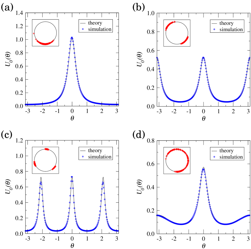
Figure 1: Stuart-Landau oscillators. (a) Synchronized, (b) 2-cluster, (c) 3-cluster, and (d) intermixed states. The insets display instantaneous distributions of the oscillators on the limit cycle.

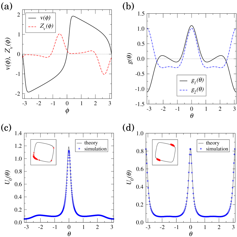
Figure 2: FitzHugh-Nagumo oscillators. (a) Variable $v(\phi)$ and phase sensitivity function $Z_{v}(\phi)$, (b) correlation functions $g_{1,2}(\theta)$ calculated from ${\bm{G}}_{1,2}({\bm{X}})$ and $Z_{v}(\phi)$, (c) synchronized state, and (d) 2-cluster state. The insets display snapshots of the oscillators.

References

• (1) Z. F. Mainen and T. J. Sejnowski, Science 268, 1503 (1995); R. F. Galรกn, N. Fourcaud-Trocmรฉ, G. B. Ermentrout, and N. N. Urban, Journal of Neuroscience 26, 3646 (2006); A. Uchida, R. McAllister, and R. Roy, Phys. Rev. Lett. 93, 244102 (2004); K. Yoshida, K. Sato, A. Sugamaga, J. Sound and Vibration 290, 34 (2006); I. Z. Kiss, J. L. Hudson, J. Escalona, and P. Parmananda, Phys. Rev. E 70, 026210 (2004) ; C. Zhou and J. Kurths, Phys. Rev. Lett. 88, 230602-1 (2002) ; T. Zhou, L. Chen, and K. Aihara, Phys. Rev. Lett. 95, 178103 (2005).
• (2) R. V. Jensen, Phys. Rev. E. 58, R6907 (1998); K. Pakdaman, Neural Comput. 14, 781 (2002); B. Gutkin, G. B. Ermentrout, and M. Rudolph, J. Comput. Neurosci. 15, 91 (2003); J. Ritt, Phys. Rev. E 68, 041915 (2003).
• (3) J. N. Teramae and D. Tanaka, Phys. Rev. Lett. 93, 204103 (2004); Prog. Theoret. Phys. Suppl. 161, 360 (2006).
• (4) D. S. Goldobin and A. Pikovsky, Phys. Rev. E 71, 045201(R) (2005); Physica A 351, 126 (2005); Phys. Rev. E 73, 061906 (2006).
• (5) K. Nagai, H. Nakao, and Y. Tsubo, Phys. Rev. E 71, 036217 (2005); H. Nakao et al., Phys. Rev. E 72, 026220 (2005); H. Nakao, K. Nagai, and K. Arai, Prog. Theoret. Phys. Suppl. 161, 294 (2006).
• (6) Y. Kuramoto, Chemical Oscillations, Waves, and Turbulence (Springer-Verlag, Berlin, 1984).
• (7) G. B. Ermentrout and N. Kopell, Journal of Mathematical Biology 29, 195 (1991).
• (8) E. M. Izhikevich, Dynamical Systems in Neuroscience: The Geometry of Excitability and Bursting (MIT Press, Cambridge, MA, 2007)
• (9) D. Golomb, D. Hansel, B. Shraiman and H. Sompolinsky, Phys. Rev. A 45, 3516 (1992); K. Okuda, Physica D 63, 424 (1993); D. Hansel, G. Mato, and C. Meunier, Phys. Rev. E 48, 3470 (1993); H. Kori and Y. Kuramoto, Phys. Rev. E 63, 046214 (2001).
• (10) C. W. Gardiner, Handbook of Stochastic Methods (Springer, Berlin, 1997); L. Arnold, Stochastic Differential Equations: Theory and Applications (John Wiley & Sons, New York, 1974).
• (11) H. Fujisaka and T. Yamada, Prog. Theor. Phys. 74, 918 (1985); N. Platt, S. M. Hammel, and J. F. Heagy, Phys. Rev. Lett. 72, 3498 (1994); S. C. Venkataramani, T. M. Antonsen, Jr., E. Ott, and J. C. Sommerer, Physica D 96, 66 (1996); H. Nakao, Phys. Rev. E 58, 1591 (1998).
• (12) When only concerned with overall distribution of the phase differences, effect of small dispersion in oscillator characteristics is qualitatively similar to introduction of independent noises in Eq.ย (1). Here, we do not treat such dispersion for simplicity.
• (13) For Gaussian processes, finite-distance jump probability in interval $\Delta t$ goes to 00 faster than $\Delta t$ as $\Delta t\to 0$ (Lindeberg conditionย SDE ), so as long as noise intensities $D$ and $\epsilon$ are sufficiently small, the trajectory of each oscillator is almost always near unperturbed limit cycle, so that phase approximation Eq.ย (2) is valid.
• (14) This intermittent transition is also induced by the noise, which is different from the dynamical intermittency caused by the intricate phase-space structure analyzed inย Clustering , and thus exhibits different statistics.
Refer to caption