Spatial Characteristics of Joint Application Networks in Japanese Patents

Abstract

Technological innovation has extensively been studied to make firms sustainable and more competitive. Within this context, the most important recent issue has been the dynamics of collaborative innovation among firms. We therefore investigated a patent network, especially focusing on its spatial characteristics. The results can be summarized as follows. (1) The degree distribution in a patent network follows a power law. A firm can then be connected to many firms via hubs connected to the firm. (2) The neighbors’ average degree has a null correlation, but the clustering coefficient has a negative correlation. The latter means that there is a hierarchical structure and bridging different modules may shorten the paths between the nodes in them. (3) The distance of links not only indicates the regional accumulations of firms, but the importance of time it takes to travel, which plays a key role in creating links. (4) The ratio of internal links in cities indicates that we have to consider the existing links firms have to facilitate the creation of new links.

, ,

1 Introduction

Technological innovation has extensively been studied to make firms sustainable and more competitive. The most important recent issue has been the dynamics of collaborative innovation among firms [1]. Moreover, a lot of countries are promoting industrial cluster policies that facilitate collaborative innovation among firms in specific regions, and emphasizing that the key is creating networks among firms. However, studying industrial clusters based on networks of firms is not sufficient because of the difficulty of obtaining comprehensive linkage data.

There have been numerous extensive studies on innovation in the social science based on networks [2]. However, these studies have focused on the details of specific collaborative innovations, and have only treated one thousand firms at most. All regional firms and their networks should be studied to enable industrial clusters to be discussed, and the firms should number more than ten thousand.

This paper focuses on networks generated by joint applications of patents in Japan. These networks can cover all Japanese firms, and these enable us to study industrial clusters. Joint applications are common in Japan, even though they are not popular in Europe or the United States. This is why there have been no similar studies in those areas.

The entire dynamics of collaborative innovation cannot be observed by focusing on the joint applications of patents. This is because all innovation is not revealed in patents, and all patents cannot lead to innovation. However, this problem can be ignored. Since exact distinctions, whether various patents have contributed to innovation do not matter, we pay attention to the structure of innovation network among firms using the patent network.

This paper is organized as follows. Section 2 explains the patent data discussed in this paper and joint application networks derived from them. In Section 3, we discuss spatial characteristics that are important for industrial clusters, and conclude this paper.

2 Japanese patent data and joint application networks

The Japanese Patent Office publishes patent gazettes, which are called Kokai Tokkyo Koho (Published Unexamined Patent Applications) and Tokkyo Koho (Published Examined Patent Applications). These gazettes are digitized, but not organized because they do not trace changes in trade name or firms’ addresses. To solve these problems, Tamada et al. has organized a database [3] and this paper is based on theirs. It includes 4,998,464 patents published from January 1994 to December 2003 in patent gazettes.

The industrial cluster program of Japan began in April 2003 but preparatory steps had not been done until March 2005. Hence, these patent data indicate a situation where the industrial cluster program had not yet affected firms. This means that we can study the innate characteristics of firms without the program having an effect, and discuss a preferable plan as to how to take advantage of the characteristics.

We extracted applicants’ data from the front pages of patents and obtained a joint application network (called a patent network after this). A patent network has applicants as nodes, and joint applications as links (Fig. 1). The links do not have weight or directions. The applicants include firms and individuals. However, the objective of this paper is to discuss what an industrial cluster should be. We hence need a patent network that only consists of firms. We consequently removed the nodes of individuals and the links they had from the patent network.

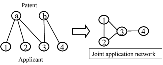
Figure 1: Examples outlining how a joint application network is created. In the figure at left, there is patent ‘a’ that has applicants ‘1’, ‘2’, and ‘3’ and ‘b’ that has ‘3’ and ‘4’. Nodes are applicants in a joint application network. Applicants are connected to each other if they apply for a patent together. There is a joint application network in the figure at right.

How to develop a local network is a key issue in discussing an industrial cluster. However, analyses of the entire network can also contribute to this. Therefore, we will discuss analyses of the entire network in the rest of this section, particularly, the basic properties of the patent network, the degree distribution, the neighbors’ average degree, and the clustering coefficient.

The largest connected component is a part of the network where all nodes can traverse each other, and which has the largest number of nodes. A network with all nodes has 67,659 nodes and 111,860 links, and the largest connected component has 34,830 nodes and 84,843 links, which represent approximately 51% and 76% of the network with all nodes, respectively.

Here, let us give a definition of measurements. The degree is the number of links a node has. If a node, i, has k links, the degree of node i is k. The clustering coefficient [4] is the measurement of triangles a node has. Node i’s clustering coefficient is quantified by $C_{i}=2e_{i}/k(k-1)$ where $k$ is the degree and $e_{i}$ is the number of links connecting the $k$ neighbors to each other. The path length is the minimum number of links we need to travel between two nodes.

The average path length is 4.45 and the longest path length is 18 in the largest connected component. The average path length and the longest path length are based on all the combination of nodes in the network. We will discuss the possibility of reducing these path lengths in the latter part of this section. The clustering coefficient of the network with all nodes is 0.29 and one of the largest connected component is 0.31. The clustering coefficient here is the average of all nodes included in the network. The clustering coefficient of other firms’ networks are smaller than this. For example, the clustering coefficient of a firms’ transaction network is 0.21 [5]. Generally, patent-network links are sparse compared to those for other networks because joint applications cannot occur without other linkages, such as alliances, and transactions. This means firms especially tend to form groups in a patent network. We will take a closer look at the clustering coefficient in the latter part of this section.

Figure 2: Degree distribution. Broken line is given by $p(k)\propto k^{-\gamma}$ with $\gamma=2.36$.

Figure 2 plots the degree distribution of the network of all nodes. The horizontal axis represents the degree, $k$, and the vertical axis indicates the cumulative distribution, which is given by $P(k)=\int_{k}^{\infty}dk\ p(k)$, where $p(k)$ means the degree distribution. If $p(k)\propto k^{-\gamma}$, $P(k\leq)\propto k^{-(\gamma-1)}$. The broken line in the figure is given by $p(k)\propto k^{-\gamma}$ with $\gamma=2.36$. From the line, we can see that the degree distribution follows a power law. This means that the patent network can be categorized as a scale-free network.

The average path length in a scale-free network follows $\mbox{log}\,\mbox{log}\,N$, where $N$ is the number of nodes. This means that nodes can reach many other nodes by traveling a few steps. If a node is connected to nodes that can reach in two links in the patent network, the average degree is 104.7 times larger than the one of the original network. Creating new links is an important issue to promote industrial clusters. Since, intuitively, connecting firms that do not have any relation is difficult, this result means that connecting firms connected to the same hub (a node with a large degree) can provide good opportunities.

We will next discuss the neighbors’ average degree. Calculating the degree correlation is one of useful measurements to discuss a network structure [6]. This is represented by conditional probability $p_{c}(k^{\prime}|k)$, the probability that a link belonging to a node with degree $k$ will be connected to a node with degree $k^{\prime}$. If this conditional probability is independent of $k$, the network has a topology without any correlation between the nodes’ degree. That is, $p_{c}(k^{\prime}|k)=p_{c}(k^{\prime})\propto k^{\prime}p(k^{\prime})$. In contrast, the explicit dependence on $k$ reveals nontrivial correlations between nodes’ degree, and the possible presence of a hierarchical structure in the network. The direct measurement of the $p_{c}(k^{\prime}|k)$ is a rather complex task due to the large number of links. More useful measurement is $<\!k_{nn}\!>=\sum_{k^{\prime}}{k^{\prime}p_{c}(k^{\prime}|k)}$, i.e., the neighbors’ average degree of nodes with degree $k$. Figure 4 shows the average degree of the network of all nodes. The horizontal axis shows the degree $k$, and the vertical axis shows the degree correlation $<\!k_{nn}\!>$. Figure 4 has a null correlation. Therefore, we cannot see the presence of a hierarchical structure for the degree in the network. If a hierarchical structure exists, there is the possibility that we can reduce the length between nodes by creating a shortcut. From the point of view of industrial clusters, reducing the length between firms is important for creating new links. However, this result for the neighbors’ average degree denies such a possibility.

We will now discuss the clustering coefficient. Its definition has already been given, and the average clustering coefficient for all nodes has also been presented. Figure 4 shows the average clustering coefficient for the network of all nodes with degree $k$. The horizontal axis indicates degree $k$, and the vertical axis represents the average clustering coefficient, $C(k)$, of all nodes with degree $k$. There seems to be a negative correlation. If a scale-free network has $C(k)\propto k^{-1}$, the network is hierarchically modular [8]. This hierarchical structure is different to the one of degree, which was previously discussed. The hierarchical structure here means that sparsely connected nodes are part of highly clustered areas, with communication between different highly clustered neighbors being maintained by a few hubs. This means that a node may have to traverse redundant hubs to access nodes in other modules. Reducing the length between firms in industrial clusters is important for creating new links. Therefore, bridging firms in different modules directly may positively affect the interactions between them.

Figure 3: Average degree $<\!k_{nn}\!>$. This figure shows nearest neighbors’ average degree of nodes with degree $k$.

Figure 4: Clustering coefficient $C(k)$. This figure shows average clustering coefficient of all nodes with degree $k$.

3 Spatial characteristics of patent networks

A lot of countries regard the regional accumulation of firms’ interactions as important in policies of industrial clusters. This section discusses the spatial characteristics of the patent network.

Figure 5 plots the frequency of distance for all links. The horizontal axis represents the geodesic distance, and the vertical axis indicates the frequency. The distance between each link is based on the nodes’ addresses connected by the link. The addresses are converted to pairs of latitudes and longitudes, and the geodesic distance is calculated from these.

There are several peaks. The largest one is around the first 10 km. The peak means that the nearer the firms, the more likely they are to have links. This supports the assumption of policies on industrial clusters because regional accumulation can be seen as a natural behavior of firms. However, there are other peaks. These are around 130 km, 250 km, and 400 km. The cause of these peaks seems to be that there are cities connected by Shinkansen (bullet train). Japan has a well organized infrastructure for public transportation, hence cities at long distances can have many links. This indicates that geographic adjacency is not the exact reason for the facilitation of links, but the time it takes to travel. If it takes a short time to travel between firms, they are likely to have links. Consequently, the infrastructure for public transportation should be considered to discuss industrial clusters at least in Japan.

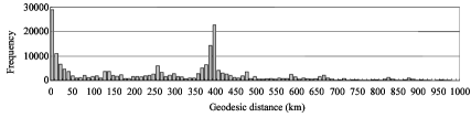
Figure 5: Frequency of distance. Distance between each link is calculated by nodes’ addresses connected by link. There are several peaks in this chart.

Figure 6: Average link ratio, $\overline{r_{k}}$. There are negative correlations in each city.

We will now define the inner link ratio of a node in a specific city as $r_{k}=k_{inside}/k$, where $k$ is degree, and $k_{inside}$ is the number of links connected to nodes in the same city. The average link ratio, $\overline{r_{k}}$, is an average of $r_{k}$ over all nodes in the same city with degree $k$. We picked out four cities that include numerous firms. They were Tokyo 23 special-wards (a primary area of the capital), Osaka, Kyoto, and Nagoya. Figure 6 shows the average link ratio for all four cities. The horizontal axis indicates the degree $k$, and the vertical axis represents the average link ratio, $\overline{r_{k}}$.

There are negative correlations in all four cities. This means that a node with a small degree prefers to have links with nodes in the same region. However, a node with a large degree tends to have links with nodes in other regions. It is thus not appropriate to adhere to create links among firms in the same region in a discussion on industrial clusters, and we should consider links that firms already have.

Summing up, the patent network reveals valuable indications of industrial cluster policies. The indications can be summarized as follows. (1) A firm can be connected to many nodes via hubs. (2) Bridging different modules may shorten the paths between nodes in them. (3) The distance between links reveals the importance of the time it takes to travel. (4) We have to consider the existing links firms have to facilitate the creation of new links.

References

- [1] M.E. Porter, On Competition, Harvard Business School Publishing, Boston, 1998.
- [2] W.W. Powell, S. Grodal, in: J. Fagerberg, D.C. Mowery, R.R. Nelson (Eds.), The Oxford Handbook of Innovation, Oxford University Press, Oxford, 2006, pp. 56-85.
- [3] S. Tamada, et al., Scientometrics 68 (2006) 289-302.
- [4] D.J. Watts, S.H. Strogatz, Nature 393 (1998) 440-442.
- [5] W. Souma, et al., Physica A 370 (2006) 151-155.
- [6] R. Pastor-Satorras, A. Vzques, A. Vespignani, Phys. Rev. Let. 87 (2001) 258701.
- [7] E. Ravasz, et al., Science 297 (2002) 1551-1555.
- [8] A.L. Barabsi, Z.N. Oltvai, Nature Reviews Genetics 5 (2004) 101-113.