Thermal Operator and Dispersion Relation in QED at Finite Temperature and Chemical Potential

Abstract

Combining the thermal operator representation with the dispersion relation in QED at finite temperature and chemical potential, we determine the complete retarded photon self-energy only from its absorptive part at zero temperature. As an application of this method, we show that, even for the case of a nonzero chemical potential, the temperature dependent part of the one loop retarded photon self-energy vanishes in $(1+1)$ dimensional massless QED.

In a series of recent papers silvana ; silvana1 ; das ; das1 , we have shown how the thermal operator representation espinosa ; silvana2 ; silvana3 , which relates a Feynman graph at finite temperature to the corresponding one at zero temperature both in the imaginary time formalism kapusta ; lebellac as well as in the real time formalism of closed time path dasbook , can be used profitably to study various questions of interest at finite temperature. For example, using thermal operator representation, the cutting rules at finite temperature and chemical potential can be directly obtained silvana and the miraculous cancellations observed earlier bedaque ; dasbook can be easily understood. The thermal operator representation also clarifies the meaning of the forward scattering amplitude description for the retarded amplitudes at finite temperature silvana1 by relating them to the corresponding forward scattering description at zero temperature. The method also allows us das to use the Schwinger proper time method schwinger to derive the hard thermal loop effective actions braaten ; frenkel in a simple manner. Furthermore, this approach clarifies the origin of many of the distinguishing features of hard thermal loop effective actions in gauge theories by tracing these properties directly to the corresponding zero temperature theory das1 .

In this brief report, we present yet another example of how the thermal operator representation can be combined with other powerful tools in quantum field theory to obtain nontrivial results at finite temperature and chemical potential. Specifically, we will show that when combined with dispersion relations, the thermal operator representation can lead directly to the complete retarded self-energy at finite temperature and chemical potential from a knowledge of only the absorptive part of the retarded self energy at zero temperature. Although this can be done for any theory, we will restrict ourselves to the retarded photon self-energy in QED which is of much interest in the study of linear response theory kapusta ; lebellac .

Dispersion relations have been studied extensively at zero temperature bjorken . For a retarded function $f(t)=\theta(t)f(t)$, the dispersion relations arise from the fact that the function in the Fourier transformed space can be written as

$$f(\omega,\vec{p}\,)=\frac{1}{2\pi i}\int d\omega^{\prime}\ \frac{f(\omega^{\prime},\vec{p}\,)}{\omega^{\prime}-\omega-i\epsilon},$$ (1)

which leads to the relations between the real and the imaginary parts as

$${\rm Re}\ f(\omega,\vec{p}\,) = \frac{1}{\pi}\int d\omega^{\prime}\ \frac{{\rm Im}\ f(\omega^{\prime},\vec{p}\,)}{\omega^{\prime}-\omega},$$

$${\rm Im}\ f(\omega,\vec{p}\,) = -\frac{1}{\pi}\int d\omega^{\prime}\ \frac{{\rm Re}\ f(\omega^{\prime},\vec{p}\,)}{\omega^{\prime}-\omega}.$$ (2)

These relations, which are conventionally known as the dispersion relations, can also be combined into one single relation

$$f(\omega,\vec{p}\,)=\frac{1}{\pi}\int d\omega^{\prime}\ \frac{{\rm Im}\ f(\omega^{\prime},\vec{p}\,)}{\omega^{\prime}-\omega-i\epsilon},$$ (3)

which determines the complete retarded amplitude at zero temperature from a knowledge of only its absorptive part. Of course, relations (2) and (3) are meaningful only if ${\rm Im}f(\omega,\vec{p}\,)$ vanishes for large values of $\omega$. If it does not, one can have a subtracted relation (for simplicity of notation, we will suppress the momentum arguments which should be understood)

$$\left(f(\omega)-f(\omega_{0})\right) = \frac{1}{\pi}\int d\omega^{\prime}\left({\rm Im}(f(\omega^{\prime})-f(\omega_{0})\right)$$ (4)

$$\times\left[\frac{1}{\omega^{\prime}-\omega-i\epsilon}-\frac{1}{\omega^{\prime}-\omega_{0}-i\epsilon}\right]\!\!,$$

where $\omega_{0}$ is an arbitrary subtraction point that is normally chosen to be $\omega_{0}=0$ in the absence of a chemical potential.

We note, however, that for the purposes of a thermal operator representation, only an unsubtracted relation such as in (3) will suffice. This is easily seen from the fact that the thermal operator acts at the integrand level before the integration over internal momenta are carried out espinosa ; silvana2 ; silvana3 . Since the absorptive part of the self-energy involves a combination of delta functions with the external energy $\omega$ as one of the arguments (it represents an on-shell process), for a fixed value of the internal momentum, it vanishes for large values of $\omega$ (the divergences arise only when the internal momenta are integrated). The important thing to note is that the thermal operator, which relates the finite temperature graphs to the zero temperature ones, is real and, consequently, it maintains the real and the imaginary nature of parts of an amplitude. Therefore, if $f(\omega)=\varPi_{\rm R}^{(0,\mu)}(\omega)$ represents the retarded self-energy in a theory at zero temperature and nonzero chemical potential $\mu$ at the integrand level (before the internal momentum integrations are done), then by applying the thermal operator, the dispersion relation at finite temperature and nonzero chemical potential follows from (3) to be (we are suppressing the momentum arguments for simplicity)

$$\varPi_{\rm R}^{(T,\mu)}(\omega)=\frac{1}{\pi}\int d\omega^{\prime}\ \frac{{\rm Im}\ \varPi_{\rm R}^{(T,\mu)}(\omega^{\prime})}{\omega^{\prime}-\omega-i\epsilon},$$ (5)

where we have identified

$$\varPi_{\rm R}^{(T,\mu)}(\omega) = {\cal O}^{(T,\mu)}\varPi_{\rm R}^{(0,\mu)}(\omega),$$

$${\rm Im}\ \varPi_{\rm R}^{(T,\mu)}(\omega) = {\cal O}^{(T,\mu)}{\rm Im}\ \varPi_{\rm R}^{(0,\mu)}(\omega),$$ (6)

with ${\cal O}^{(T,\mu)}$ denoting the appropriate thermal operator for the amplitude silvana2 ; silvana3 . This generalizes the dispersion relation (3) at zero temperature to that at finite temperature and chemical potential. Furthermore, through the use of the dispersion relation and the thermal operator, this method shows how the complete retarded self-energy at finite temperature and chemical potential can be obtained from a knowledge of only the absorptive part of the zero temperature retarded self-energy.

Let us now demonstrate how this works in QED with a nonzero chemical potential $\mu$ by calculating the retarded self-energy for the photon. The Lagrangian density for the theory is given by

$${\cal L}=-\frac{1}{4}F_{\mu\nu}F^{\mu\nu}+i\bar{\psi}D\!\!\!\!/\psi-m\bar{\psi}\psi+\mu\bar{\psi}\gamma^{0}\psi,$$ (7)

where $D_{\mu}$ denotes the covariant derivative and $F_{\mu\nu}$ is the Abelian field strength tensor. In the closed time path formalism, the propagator in the mixed space becomes a $2\times 2$ matrix and at zero temperature has the form silvana2

$$iS_{++}^{(0,\mu)}(t,\vec{p}\,) = \frac{e^{i\mu t}}{2E_{p}}\left(\theta(t)A(E_{p})e^{-iE_{p}t}+\theta(-t)B(E_{p})e^{iE_{p}t}\right),\quad iS_{+-}^{(0,\mu)}(t,\vec{p}\,)=\frac{e^{i\mu t}}{2E_{p}}\ B(E_{p})e^{iE_{p}t},$$

$$iS_{-+}^{(0,\mu)}(t,\vec{p}\,) = \frac{e^{i\mu t}}{2E_{p}}\ A(E_{p})e^{-iE_{p}t},\quad iS_{--}^{(0,\mu)}(t,\vec{p}\,)=\frac{e^{i\mu t}}{2E_{p}}\left(\theta(t)B(E_{p})e^{iE_{p}t}+\theta(-t)A(E_{p})e^{-iE_{p}t}\right),$$ (8)

where

$$E_{p}=\sqrt{\vec{p}^{2}+m^{2}},\quad A(E_{p})=\gamma^{0}E_{p}-\vec{\gamma}\cdot\vec{p}=\gamma^{\mu}A_{\mu}(E_{p}),\quad B(E_{p})=-\gamma^{0}E_{p}-\vec{\gamma}\cdot\vec{p}=\gamma^{\mu}B_{\mu}(E_{p}).$$ (9)

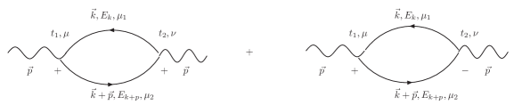
Figure 1: The two diagrams contributing to the retarded self-energy for the photon at one loop.

The retarded one loop self-energy for the photon (see Fig. 1) can now be calculated easily. We note here that since the chemical potential occurs as a phase in the components of the propagator in (8), in the contribution of the fermion loop to the self-energy at zero temperature, the dependence on the chemical potential will cancel out. However, as explained in silvana3 , for purposes of applying the thermal operator, we assign distinct chemical potentials $\mu_{1},\mu_{2}$ to the two fermion propagators in the loop and identify $\mu_{1}=\mu_{2}=\mu$ only at the end. This simplifies and makes unambiguous the effect of the thermal operator. In $n$ dimensions in the mixed space, the retarded photon self-energy at zero temperature has the form (unfortunately, both the vector index of the polarization tensor as well as the chemical potential are conventionally labelled $\mu$, but we do not believe this will cause any confusion)

$$\Pi_{\rm R}^{\mu\nu(0,\mu)}(t_{1}-t_{2},\vec{p})=\int\frac{d^{n-1}k}{(2\pi)^{n-1}}\ \varPi_{\rm R}^{\mu\nu(0,\mu)}(t_{1}-t_{2},\vec{p},\vec{k}),$$ (10)

where

$$\varPi_{\rm R}^{\mu\nu(0,\mu)}(t_{1}-t_{2},\vec{p},\vec{k})=\frac{ine^{2}}{4E_{k}E_{k+p}}\ \theta(t_{1}-t_{2})e^{-i(\mu_{1}-\mu_{2})(t_{1}-t_{2})}\left[N^{\mu\nu}e^{-i(E_{k}+E_{k+p})(t_{1}-t_{2})}-M^{\mu\nu}e^{i(E_{k}+E_{k+p})(t_{1}-t_{2})}\right],$$ (11)

with

$$N^{\mu\nu}(E_{k},E_{k+p}) = A^{\mu}(E_{k+p})B^{\nu}(E_{k})-\eta^{\mu\nu}(A(E_{k+p})\cdot B(E_{k})-m^{2})+A^{\nu}(E_{k+p})B^{\mu}(E_{k}),$$

$$M^{\mu\nu}(E_{k},E_{k+p}) = B^{\mu}(E_{k+p})A^{\nu}(E_{k})-\eta^{\mu\nu}(B(E_{k+p})\cdot A(E_{k})-m^{2})+B^{\nu}(E_{k+p})A^{\mu}(E_{k}).$$ (12)

Equation (11) can now be Fourier transformed in the external time variables to yield ($\omega$, which represents the external energy, is the variable of Fourier transformation and we will suppress the arguments $\vec{p},\vec{k}$ in the self-energy for simplicity)

$$\varPi_{\rm R}^{\mu\nu(0,\mu)}(\omega) = \frac{ne^{2}}{4E_{k}E_{k+p}}\left[-\frac{N^{\mu\nu}}{\omega-E_{k}-\mu_{1}-E_{k+p}+\mu_{2}+i\epsilon}+\frac{M^{\mu\nu}}{\omega+E_{k}-\mu_{1}+E_{k+p}+\mu_{2}+i\epsilon}\right],$$ (13)

$${\rm Im}\ \varPi_{\rm R}^{\mu\nu(0,\mu)}(\omega) = \frac{n\pi e^{2}}{4E_{k}E_{k+p}}\left[N^{\mu\nu}\delta(\omega-E_{k}-\mu_{1}-E_{k+p}+\mu_{2})-M^{\mu\nu}\delta(\omega+E_{k}-\mu_{1}+E_{k+p}+\mu_{2})\right].$$ (14)

It is clear now that, for a fixed finite value of $\vec{k}$, ${\rm Im}\ \varPi_{\rm R}^{\mu\nu(0.\mu)}(\omega)$ vanishes for large values of $\omega$ and that (14) and (13) satisfy the zero temperature dispersion relation (3). If we are only interested in the zero temperature result, we can set $\mu_{1}=\mu_{2}=\mu$ at this point, which will lead to the result that the absorptive part of the retarded self-energy and, therefore, the full retarded self-energy, at zero temperature do not depend on the chemical potential, which is more directly seen from the mixed space result in (11) (by setting $\mu_{1}=\mu_{2}=\mu$).

As pointed out in (6), at finite temperature, the imaginary part of the retarded self-enrgy can be obtained through the application of the thermal operator, which in the present case takes the form

$${\cal O}^{(T,\mu)} = \left(1-\hat{N}_{\rm F}^{(T,\mu_{1})}(E_{k})(1-S(E_{k}))\right)$$ (15)

$$\times \left(1-\hat{N}_{\rm F}^{(T,\mu_{2})}(E_{k+p})(1-S(E_{k+p}))\right),$$

where $S(E)$ is a reflection operator that changes $E\rightarrow-E$ and $\hat{N}_{\rm F}^{(T,\mu)}(E)$ denotes a fermion distribution operator whose action is described in silvana3 . Applying the thermal operator (15), we obtain

$${\rm Im}\ \varPi_{\rm R}^{\mu\nu(T,\mu)}(\omega) = \frac{n\pi e^{2}}{4E_{k}E_{k+p}}\left[\delta(\omega-E_{k}-E_{k+p})\left(1-n_{\rm F}^{+}(E_{k})-n_{\rm F}^{-}(E_{k+p})\right)N^{\mu\nu}\right.$$

$$- \delta(\omega+E_{k}+E_{k+p})\left(1-n_{\rm F}^{-}(E_{k})-n_{\rm F}^{+}(E_{k+p})\right)M^{\mu\nu}$$

$$- \left.\delta(\omega+E_{k}-E_{k+p})\left(n_{\rm F}^{-}(E_{k})-n_{\rm F}^{-}(E_{k+p})\right)\bar{N}^{\mu\nu}+\delta(\omega-E_{k}+E_{k+p})\left(n_{\rm F}^{+}(E_{k})-n_{\rm F}^{+}(E_{k+p})\right)\bar{M}^{\mu\nu}\right],$$

where we have used the standard notation $n_{\rm F}^{\pm}(E)=n_{\rm F}(E\pm\mu)$ and have defined

$$\bar{N}^{\mu\nu} = N^{\mu\nu}(-E_{k},E_{k+p})=A^{\mu}(E_{k+p})A^{\nu}(E_{k})-\eta^{\mu\nu}(A(E_{k+p})\cdot A(E_{k})-m^{2})+A^{\nu}(E_{k+p})A^{\mu}(E_{k}),$$

$$\bar{M}^{\mu\nu} = M^{\mu\nu}(-E_{k},E_{k+p})=B^{\mu}(E_{k+p})B^{\nu}(E_{k})-\eta^{\mu\nu}(B(E_{k+p})\cdot B(E_{k})-m^{2})+B^{\nu}(E_{k+p})B^{\mu}(E_{k}).$$ (17)

The appearance of new channels of reaction at finite temperature is manifest in the absorptive part in (Thermal Operator and Dispersion Relation in QED at Finite Temperature and Chemical Potential) and has been obtained here from the zero temperature result through the thermal operator representation. We note here that while at zero temperature, the imaginary part of the retarded photon self-energy leads to the probability for the decay of the photon, at finite temperature, the additional channels represent the scattering of thermal fermions by a photon, which become dominant at very high temperatures (in the hard thermal loop approximation).

Using the finite temperature dispersion relation in (5), we can now determine the full retarded self-energy for the photon at finite temperature and chemical potential from (Thermal Operator and Dispersion Relation in QED at Finite Temperature and Chemical Potential) to be

$$\varPi_{\rm R}^{\mu\nu(T,\mu)}(\omega) = -\frac{ne^{2}}{4E_{k}E_{k+p}}\left[\frac{(1-n_{\rm F}^{+}(E_{k})-n_{\rm F}^{-}(E_{k+p}))N^{\mu\nu}}{\omega-E_{k}-E_{k+p}+i\epsilon}-\frac{(1-n_{\rm F}^{-}(E_{k})-n_{\rm F}^{+}(E_{k+p}))M^{\mu\nu}}{\omega+E_{k}+E_{k+p}+i\epsilon}\right.$$ (18)

$$\qquad\left.-\frac{(n_{\rm F}^{-}(E_{k})-n_{\rm F}^{-}(E_{k+p}))\bar{N}^{\mu\nu}}{\omega+E_{k}-E_{k+p}+i\epsilon}+\frac{(n_{\rm F}^{+}(E_{k})-n_{\rm F}^{+}(E_{k+p}))\bar{M}^{\mu\nu}}{\omega-E_{k}+E_{k+p}+i\epsilon}\right].$$

This demonstrates how starting from only the absorptive part of the retarded self-energy at zero temperature, we can obtain the full retarded self-energy at finite temperature and chemical potential through the use of the dispersion relation and the application of the thermal operator. For $n=4$, Eq. (18) reduces to the well known result in QED silvana3 ; kapusta ; lebellac . We note here that both (Thermal Operator and Dispersion Relation in QED at Finite Temperature and Chemical Potential) as well as (18) are non-analytic at the origin in the energy-momentum space because of the additional channels of reaction. The non-commuting nature of the limits $\omega\rightarrow 0,\vec{p}\rightarrow 0$ and $\vec{p}\rightarrow 0,\omega\rightarrow 0$ arises because they represent different physical effects at finite temperature. However, for $\vec{p}\neq 0$, the retarded self-energy $\Pi_{\rm R}^{\mu\nu(T,\mu)}(\omega)$ is an analytic function in the entire upper half of the complex $\omega$-plane which justifies the dispersion relation in (5).

Let us next consider the Schwinger model schwinger1 which corresponds to two dimensional massless QED. For $m=0$, in two dimensions ($n=2$) we have various simplifications. First, we can write

$$E_{k}=|k^{1}|,\quad E_{k+p}=|k^{1}+p^{1}|.$$ (19)

Furthermore, in two dimensions the tensors in (12) and (17) simplify to have the forms

$$N^{\mu\nu} = -2E_{k}E_{k+p}\left[\theta(k^{1})\theta(-k^{1}-p^{1})u^{\mu}_{+}u^{\nu}_{+}+\theta(-k^{1})\theta(k^{1}+p^{1})u^{\mu}_{-}u^{\nu}_{-}\right],$$

$$M^{\mu\nu} = -2E_{k}E_{k+p}\left[\theta(-k^{1})\theta(k^{1}+p^{1})u^{\mu}_{+}u^{\nu}_{+}+\theta(k^{1})\theta(-k^{1}-p^{1})u^{\mu}_{-}u^{\nu}_{-}\right],$$

$$\bar{N}^{\mu\nu} = 2E_{k}E_{k+p}\left[\theta(-k^{1})\theta(-k^{1}-p^{1})u^{\mu}_{+}u^{\nu}_{+}+\theta(k^{1})\theta(k^{1}+p^{1})u^{\mu}_{-}u^{\nu}_{-}\right],$$

$$\bar{M}^{\mu\nu} = 2E_{k}E_{k+p}\left[\theta(k^{1})\theta(k^{1}+p^{1})u^{\mu}_{+}u^{\nu}_{+}+\theta(-k^{1})\theta(-k^{1}-p^{1})u^{\mu}_{-}u^{\nu}_{-}\right],$$ (20)

where we have defined the null vectors

$$u^{\mu}_{+}=(1,-1),\quad u^{\mu}_{-}=(1,1).$$ (21)

With the relations (19) and (20), the temperature dependent part of ${\rm Im}\ \varPi_{\rm R}^{\mu\nu(T,\mu)}(\omega)$ in (Thermal Operator and Dispersion Relation in QED at Finite Temperature and Chemical Potential) can be simplified and takes the form (we use the standard notation dasbook ; adilson $A^{(T)}=A^{(0)}+A^{(\beta)}$ decomposing any observable to its zero temperature part and the temperature dependent part)

$${\rm Im}\ \varPi_{\rm R}^{\mu\nu(\beta,\mu)}(\omega)$$ (22)

$$= \pi e^{2}\left[\delta(\omega+p^{1})u^{\mu}_{+}u^{\nu}_{+}\left\{\theta(k^{1})n_{\rm F}^{+}(E_{k})-\theta(-k^{1})n_{\rm F}^{-}(E_{k})-\theta(k^{1}+p^{1})n_{\rm F}^{+}(E_{k+p})+\theta(-k^{1}-p^{1})n_{\rm F}^{-}(E_{k+p})\right\}\right.$$

$$+ \left.\delta(\omega-p^{1})u_{-}^{\mu}u_{-}^{\nu}\left\{\theta(-k^{1})n_{\rm F}^{+}(E_{k})-\theta(k^{1})n_{\rm F}^{-}(E_{k})-\theta(-k^{1}-p^{1})n_{\rm F}^{+}(E_{k+p})+\theta(k^{1}+p^{1})n_{\rm F}^{-}(E_{k+p})\right\}\right].$$

If we use the fact that $\varPi_{\rm R}^{\mu\nu}$ is the integrand in an integral involving $k^{1}$ for the self-energy (see, for example, (10)), we can redefine $k^{1}\rightarrow-k^{1}-p^{1}$ in some of the terms in (22) to rewrite the temperature dependent part as

$${\rm Im}\ \varPi_{\rm R}^{\mu\nu(\beta,\mu)}(\omega) = \pi e^{2}\epsilon(k^{1})\left(n_{\rm F}^{+}(E_{k})+n_{\rm F}^{-}(E_{k})\right)$$

$$\times \!\!\!\left(\delta(\omega+p^{1})u^{\mu}_{+}u^{\nu}_{+}-\delta(\omega-p^{1})u^{\mu}_{-}u^{\nu}_{-}\right),$$

where $\epsilon(k^{1})=\theta(k^{1})-\theta(-k^{1})$. The important thing to note here is that the integrand of the imaginary part of the temperature dependent retarded self-energy is anti-symmetric in the integration variable $k^{1}$ because of the alternating step function. As a result, through the dispersion relation (5), the temperature dependent part of the complete retarded self-energy, $\varPi_{\rm R}^{\mu\nu(\beta,\mu)}(\omega)$, would also inherit this anti-symmetry. It follows, therefore, that the temperature dependent imaginary part of the retarded self-energy as well as the retarded self-energy vanish (when integrated over $k^{1}$) for the Schwinger model. This result is a generalization of adilson to the case of a nonzero chemical potential. We note here that the delta function structure as well as the manifest anti-symmetry in (Thermal Operator and Dispersion Relation in QED at Finite Temperature and Chemical Potential) is a reflection of helicity conservation for massless fermions scattering from a photon background in $1+1$ dimensions.

Acknowledgment:

One of us (AD) acknowledges the Fulbright Foundation for a fellowship. This work was supported in part by US DOE Grant number DE-FG 02-91ER40685, by CNPq and by FAPESP, Brazil. We have used the program Jaxodraw binosi for generating the figure in this paper.

References

• (1) F. T. Brandt, A. Das, O. Espinosa, J. Frenkel and S. Perez, Phys. Rev. D74, 085006 (2006).
• (2) F. T. Brandt, A. Das, J. Frenkel and S. Perez, Phys. Rev. D74, 125005 (2006).
• (3) A. Das and J. Frenkel, Phys. Rev. D75, 025021 (2007).
• (4) A. Das and J. Frenkel, Hard thermal effective action in QCD through the thermal operator, hep-th/0703079.
• (5) O. Espinosa, Phys. Rev. D71, 065009 (2005).
• (6) F. T. Brandt, A. Das, O. Espinosa, J. Frenkel and S. Perez, Phys. Rev. D72, 085006 (2005); ibid D73, 065010 (2006).
• (7) F. T. Brandt, A. Das, O. Espinosa, J. Frenkel and S. Perez, Phys. Rev. D73, 067702 (2006).
• (8) J. I. Kapusta, Finite Temperature Field Theory (Cambridge University Press, Cambridge, England, 1989).
• (9) M. Le Bellac, Thermal Field Theory (Cambridge University Press, Cambridge, England, 1996).
• (10) A. Das, Finite Temperature Field Theory (World Scientific, Singapore, 1997).
• (11) P. F. Bedaque, A. Das and S. Naik, Mod. Phys. Lett. A12, 2481 (1997).
• (12) J. Schwinger, Phys. Rev. 82, 664 (1951).
• (13) E. Braaten and R. Pisarski, Nucl. Phys. B337, 569 (1990); ibid B339, 310 (1990); ibid Phys. Rev. D45, 1827 (1992).
• (14) J. Frenkel and J. C. Taylor, Nucl. Phys. B334, 199 (1990); ibid B374, 156 (1992); ibid B685, 393 (2004).
• (15) See, for example, J. D. Bjorken and S. D. Drell, Relativistic Quantum Fields, (McGraw-Hill, 1965); K. Nishijima, Field Theory and Dispersion Relations, (W. A. Benjamin, 1969).
• (16) J. Schwinger, Phys. Rev. 128, 2425 (1952).
• (17) F. T. Brandt, A. Das, J.Frenkel and A. J. Da Silva, Phys. Rev. D59, 065004 (1999); F. T. Brandt, A. Das and J. Frenkel, Phys. Rev. D60, 105008 (1999).
• (18) D. Binosi and L. Theußl, Comp. Phys. Comm. 161, 76 (2004).