The Lorentz factor distribution and luminosity function of relativistic jets in AGNs

Abstract

The observed apparent velocities and luminosities of the relativistic jets in AGNs are significantly different from their intrinsic values due to strong special relativistic effects. We adopt the maximum likelihood method to determine simultaneously the intrinsic luminosity function and the Lorentz factor distribution of a sample of AGNs. The values of the best estimated parameters are consistent with the previous results, but with much better accuracy. In previous study, it was assumed that the shape of the observed luminosity function of Fanaroff-Riley type II radio galaxies is the same with the intrinsic luminosity function of radio loud quasars. Our results prove the validity of this assumption. We also find that low and high redshift groups divided by $z=0.1$ are likely to be from different parent populations.

1 Introduction

The large scale and relativistic jets are important characteristics of active galactic nuclei (AGNs). Determining their proper velocity distribution and intrinsic luminosity function is of fundamental importance for understanding the central engine of AGNs. However, the observed apparent velocities and luminosities of the relativistic jets in AGNs are significantly different from their intrinsic values due to strong special relativistic effects, i.e. $\beta_{app}=\frac{{\beta\sin\theta}}{{1-\beta\cos\theta}}$ and $S=\frac{{L\delta^{p}}}{{4\pi d_{L}^{2}(z)}}(1+z)^{1+\alpha}$, where $\beta,\;\beta_{app},\;\theta,\;L,\;S,\;\delta\;{\rm{and}}\;d_{L}$ are the proper velocity, the apparent velocity, the angle between the axis of jet and the line of sight, the intrinsic luminosity, the observed flux, the Doppler factor and the luminosity distance, respectively. The index $p$ is equal to $n-\alpha$ , where $\alpha$ is the spectral index ($S\propto\nu^{\alpha}$) and $n=2,3$ for continuous or discrete jet, respectively.

Due to the lack of reliable and accurate methods to obtain $\beta$ or $\theta$ of each source, it remains difficult to determine directly the intrinsic luminosity and the proper velocity of a relativistic jet. Several authors have addressed these problems with statistical methods. For example, Padovani & Urry (1992) determined the evolution parameters of different types of galaxies with the $<V/V_{m}>$ method, and then used the observed luminosity function of Fanaroff-Riley type II radio galaxies (FR II) as the intrinsic luminosity function of relativistic jets in AGNs, after multiplying a constant factor. This approach is at best an approximation only, because the observed luminosity function of FR II may or may not resemble the intrinsic luminosity function of relativistic jets in AGNs. Lister & Marscher (1997) extended this work with a simulation approach by fully considering the flux limit and Doppler beaming effect. However, they utilized the parameters determined by Padovani & Urry (1992) due to the size limit of the simulation. Therefore, the above mentioned approaches could not determine simultaneously the intrinsic luminosity and Lorentz factor distribution of relativistic jets in AGNs. Actually, the observed luminosity function and the apparent velocity distribution can be reproduced if the intrinsic luminosity and the Lorentz factor distribution are given (Lister 2003, Vermeulen & Cohen 1994). Thus the intrinsic luminosity and Lorentz factor distribution could be inferred simultaneously with the maximum likelihood method. Therefore, we could test the previous assumption that the observed luminosity function of FR II has the same shape with the intrinsic luminosity function of the radio loud quasars.

The form of the maximum likelihood estimator could be written as

$$MLE=\sum\limits_{i}{C\ln p(\beta_{app,i}\;,\;L_{o,i}\;,\;z_{i})},$$

where $i$ denotes the number of each source in the sample and $p$ is the probability density of detecting a source for the given apparent velocity, observed luminosity and redshift. $C$ is the normalized factor. The probability density $p$ is

$$p(\beta_{app},L_{o},z)=f(\beta_{app}|\;L_{o},\;z)\Phi(L_{o},\;z)d_{A}(z)^{2}(1+z)^{3}c\frac{{dT(z)}}{{dz}},$$

where $\beta_{app}$, $d_{A}$, $T(z)$, $f(\beta_{app}|\;L_{o},\;z)$ and $\Phi(L_{o},z)$ are the apparent velocity, the angular distance, the look-back time, the apparent velocity distribution (for the given observed luminosity and redshift) and the observed luminosity function, respectively. As proved by Vermeulen & Cohen (1994, also see Appendix A at the end of this paper), if we assume the intrinsic luminosity function is a single power law ($\Phi(L)\propto L^{-A}$), $L_{o}$ will not appear in $f(\beta_{app}|\;L_{o},\;z)$. Therefore, we could deal with the apparent velocity distribution and the observed luminosity function separately.

We present the results obtained from the apparent velocity and the observed luminosity (also the redshift) in §2. The implication of our results for the unification scheme of radio loud AGNs is addressed in §3. In §4 we summarize our conclusions and make some discussions. The cosmological parameters adopted throughout this paper are $(H_{0},\;\Omega_{M},\;\Omega_{\Lambda})=(75\;{\rm{km/s/Mpc}},\;0.27,\;0.73)$ .

2 Sample selection and data analysis

To investigate the real parent population of the radio loud AGNs, we should adopt a large sample containing different kinds of radio loud AGNs, including radio galaxies, quasars, and blazars. The largest available sample of the kinetics of relativistic jets in AGNs is from the “VLBA 2 cm survey” (Kellermann et al. 2004). Its successor, the “MOJAVE survey ”, provides a complete flux-limited sample further. Due to the high frequency observation (15 GHz), any radio emission from large scale structures is effectively excluded. The majority of the sample are the flat-spectrum radio quasars (FSRQ), which is the most luminous type in AGNs. According to the unified model, FSRQ is the beamed version of FRII due to the small angle between the jet and the line of sight.

2.1 Analysis of the apparent velocity data

In this section we only make use of the apparent velocity data to determine the intrinsic luminosity and Lorentz factor distribution. The detailed formulae of the apparent velocity distribution are presented in Appendix A.

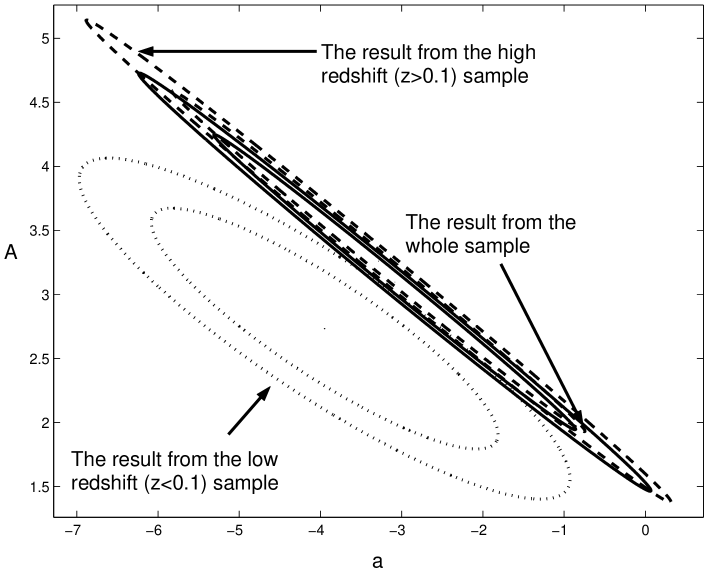
Figure 1: Inferred parameters from the apparent velocity data. The confidence regions are results obtained with the whole sample (solid lines), $z>0.1$ sources (dashed lines), and $z<0.1$ sources (dot lines), respectively. The 68% and 90% confidence regions are shown for each case.

Our sample of the apparent velocity data comes from the “VLBA 2 cm survey” (Kellermann et al. 2004). We only adopt the fastest component of each source that has a quality factor of “Good” or “Excellent” (see Figure 11 in Kellermann et al. 2004), since several authors have pointed out that the velocities of some patterns are much slower than the bulk velocity responsible for the Doppler boosting effect (Cohen et al. 2006). The sample used here contains 16 BL Lac objects, 12 radio galaxies and 76 quasars. We assume the Lorentz factor distribution is also a single power law ($p(\gamma)\propto\gamma^{a}\;(1<\gamma<\gamma_{\max})$) as adopted by previous studies. As indicated by previous studies, the maximum value of $\beta_{app}$ is nearly the same as $\gamma_{max}$ (Vermeulen & Cohen 1994). The maximum value of $\beta_{app}$ in the sample is about 31, and therefore we set $\gamma_{\max}=32$ for safety. As assumed by the previous study (Lister & Marscher 1997), we set $n=2$ and $\alpha=0$. It has been found that these simple assumptions could give reasonable results. The estimated result from the whole sample is shown in Figure 1. Obviously, the constraint on the parameters is weak, which is due to the limitation of the observed data. However, it is still useful to constrain the values of parameters with such data, because this allows us to compare between the results from the apparent velocity data and that obtained from the observed luminosity data, in order to check the consistency of our models.

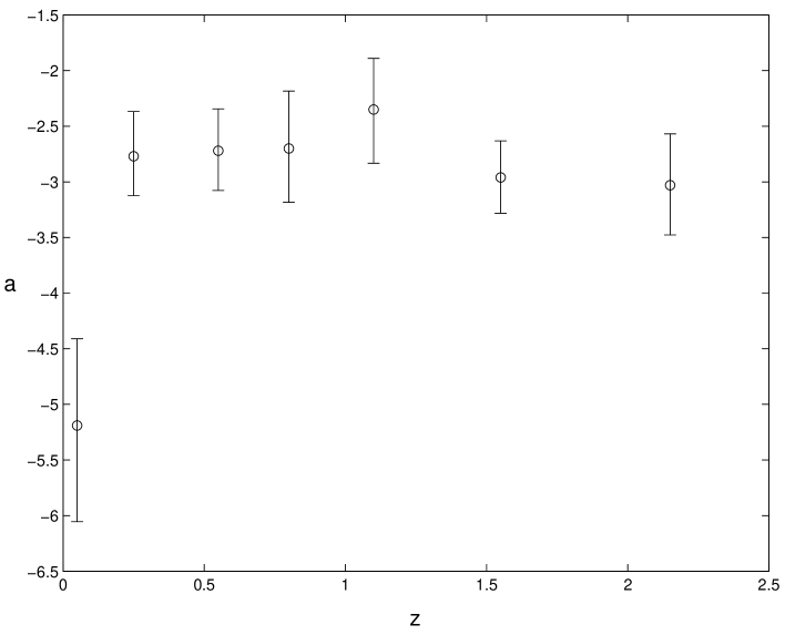
Figure 2: Evolution of the index of the Lorentz factor distribution by fixing $A=3.10$. From low to high reshift, there are 13, 17, 17, 13, 17, 17 and 10 sources in each redshift bin, respectively. The $1\sigma$ errors are shown for each redshfit bin.

By fixing the index $A$, we could investigate whether the Lorentz factor distribution evolves with the redshift. We fix $A=3.10$ (the best estimated value of $A$ for the whole sample) and estimate $a$ in each redshift bin. As shown in Figure 2, the Lorentz factor distribution is much steeper in the first bin ($0<z<0.1$) than in other bins. The difference of the apparent velocity distributions between the first bin and other bins is also significant at the 99.98% level obtained by K-S test. Therefore, we should divide the sample into low and high redshift groups by $z=0.1$. The estimated parameters of the two groups are also shown in Figure 1. The difference between the results from the whole sample and the high redshift sample is only slight, whereas the confidence region of low redshift sources differs with others at 90% confidence.

2.2 Analysis of the observed luminosity function and redshift distribution

We assume the local intrinsic luminosity function is a single power law

$$\Phi(L,\;z=0)=kL^{-A}\;\;(L_{1}\leq L\leq L_{2}),$$

and to compare with the previous results, we also assume a pure luminosity evolution model as used in Padovani & Urry (1992) and Lister & Marscher (1997),

$$\Phi(L,\;z)=\Phi(L/\exp[T(z)/\tau],\;z=0),$$

where $\tau$ is the evolution parameter in unit of Hubble time.

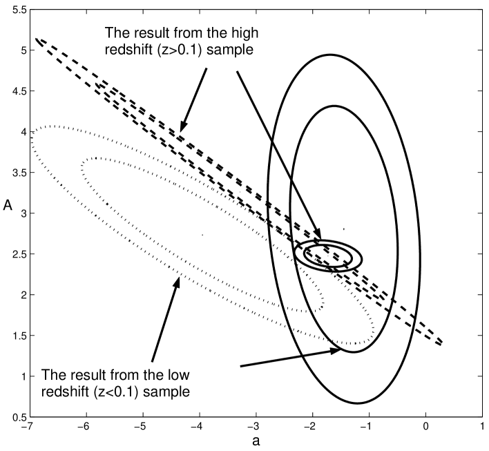
Figure 4: The results from the observed luminosity and redshift (solid lines). For comparison, the results from the apparent velocity are also shown (dashed lines). The 68% and 90% confidence regions are shown for each case.

Using the equations of the beamed luminosity function (see details in Appendix B), we can estimate the parameters in the intrinsic luminosity function, the Lorentz factor distribution and the evolution form by the maximum likelihood method. We combine the data from “VLBA 2 cm survey” and “MOJAVE survey” (Figure 3). We again divide the sample into low and high redshift groups by $z=0.1$. The values of the best estimated parameters from high redshift group are $a=-1.73_{-0.28}^{+0.28}$, $A=2.48_{-0.09}^{+0.09}$, $\tau=0.29_{-0.01}^{+0.03}$ and $\log(L_{1}({\rm{W/Hz}}))=26.25_{-0.12}^{+0.03}$; the results from the low redshift group are $a=-1.5_{-0.6}^{+0.6}$, $A=2.8_{-1.0}^{+1.0}$ and $\log(L_{1}({\rm{W/Hz}}))=24.39_{-0.40}^{+0.09}$ (no evolution is assumed for the low redshift group, and $1\sigma$ error for each parameter of concern is shown). The value of $\log(L_{2}({\rm{W/Hz}}))$ is fixed at 34, since higher values barely change the results. Figure 4 shows the confidence region for $(a,A)$ by fixing other parameters at the best estimated values. Although the confidence regions in Figure 4 for the low and high redshift groups are consistent within the 68% confidence region, the lower intrinsic luminosity limits of the two groups are different significantly. As also shown in Figure 4, the result from the luminosity data for the low redshift group is only marginally consistent with the result from the apparent velocity data within the 68% confidence region. This indicates that our current model do not describe the low redshift group very appropriately. Actually, if we adopt the whole sample, the result of the Lorentz factor distribution is unreasonable, i.e. $a>0$ is required to obtain the maximum value of the estimator, which is ruled out by previous studies. For example, if we adopt $\log(L_{1}({\rm{W/Hz}}))=24.39$ indicated by the low redshift group, the values of best estimated parameters of the whole sample are $a=30.6$, $A=3.5$ and $\tau=1.0$. The K-S test is performed to estimate the goodness of fit; the corresponding probabilities of the apparent velocity, the observed luminosity and the redshift distribution are $10^{-22}$, 10% and 7%, respectively. Therefore, the consistency is quite poor, especially for the apparent velocity. If the lower intrinsic luminosity limit is adjusted as a free parameter, the value of $a$ will become larger and even without an upper limit, which is more inconsistent with the result from the apparent velocity data. Therefore, we find that the results from both the apparent velocity and the observed luminosity data indicate the low and high redshift groups are likely to be from different parent populations. Due to the limited size of the low redshift group, we only utilize the high redshift groups in further analysis.

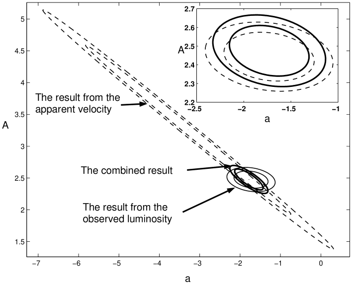
Figure 5: The thin solid lines are the results from the observed luminosity and the redshift distribution. The dashed lines are the results from the apparent velocity distribution ($z>0.1$). The thick solid lines are the combined results. The inset shows the results from the observed luminosity and the redshift distribution for $S_{min}=0.32$ (solid lines) and $S_{min}=0.50$ (dashed lines). The 68% and 90% confidence regions are shown for each case.

As shown in Figure 5, there is slight difference between the result obtained from the apparent velocity data and the observed luminosity function (within 68% confidence region). This is mainly due to the simple evolution form used here. When performing the K-S test to estimate the goodness of fit, we find the result of the best estimated value of parameters could only be accepted marginally. The corresponding probabilities of the apparent velocity, the observed luminosity and the redshift distribution are 45%, 56% and 6%, respectively. However, if we adjust the value of $\tau$ to the $1\sigma$ boundary ($\tau=0.32$), the result of K-S test could be improved. The corresponding probabilities of the apparent velocity, the observed luminosity and the redshift distribution are 45%, 61% and 20%, respectively. The effect of a higher flux limit is only mild (see the inset in Figure 4).

3 Implication for the unification scheme of radio loud AGNs

There are two key parameters in the unification scheme of radio loud AGNs. One is the orientation of the sources, and another is the intrinsic luminosity of the sources. The high luminosity population contains quasars and luminous radio galaxies (FR II), while the low luminosity population contains BL Lac objects and less luminous radio galaxies (FR I). On the other hand, the viewing angles of quasars and BL Lac objects are smaller than that of radio galaxies. Therefore, the superluminal motion is more common in the aligned objects, and the observed luminosity is strongly affected by special relativistic effects. However, the relativistic beaming effect of radio galaxies is mild and the observed luminosity function of radio galaxies is supposed to be similar to the intrinsic one. The discussion about the low luminosity population could be found in Padovaani & Urry (1990, 1991) and Urry et al. (1991), and the unification scheme was reviewed in Urry & Padovani (1995). Due to the limited sample size of low luminosity population and unclear relationship between FR I and FR II, we focus our discussion on the high luminosity population below.

Several papers investigated the luminosity function of AGNs. For example, Urry & Padovani (1995) found the evolution parameter $\tau$ of FR II and FSRQ are $0.26_{-0.10}^{+0.74}$ and $0.23_{-0.04}^{+0.07}$, respectively. Padovani & Urry (1992) adopted a double power law to fit the observed luminosity function of FR II, which was identified as the parent luminosity function. The power law indices of low and high luminosity band were found to be $B_{1}=2.48_{-0.15}^{+0.15}$ and $B_{2}=3.9_{-0.7}^{+0.7}$, respectively. Here we have determined simultaneously the intrinsic luminosity function and the Lorentz factor distribution of relativistic jets in AGNs by the maximum likelihood method. However, we find a single power law form of the intrinsic luminosity function is sufficient to describe the sample we used here. For comparison, we have re-analyzed the observed luminosity function of the FR II sample adopted in Padovani & Urry (1992) by the maximum likelihood method (for completeness, only the sources with $z<1.3$ are used). To compare with our result, we also adopt a single power law ($\Phi(L_{o},z=0)\propto L_{o}^{-A}$) and the pure luminosity evolution. The results are $A=2.51_{-0.15}^{+0.15}$ and $\tau=0.40_{-0.09}^{+0.09}$. The corresponding probabilities obtained by K-S test of the observed luminosity and the redshift distribution are 75% and 80%, respectively. Therefore, we find this simple model could describe the data well, and the result is consistent with the intrinsic luminosity function we have obtained in §2. In previous studies (Padovani & Urry 1992; Lister & Marscher 1997), it was assumed that the shape of the observed luminosity function of FR II is the same with the intrinsic luminosity function of the radio loud quasars. Therefore, our results prove the validity of this assumption. The single power law form of the luminosity function may be somewhat simplified, and a more complex form will be investigated when a larger and more complete sample is available.

4 Discussions and conclusions

We have determined simultaneously the intrinsic luminosity function and the Lorentz factor distribution of relativistic jets in AGNs by the maximum likelihood method, and have confirmed the previous assumption about the shape of the intrinsic luminosity fucntion. The result of the Lorentz factor distribution is also consistent with the previous result. For example, Lister (1997) claimed the index of the Lorentz factor distribution $a$ is roughly between -1.75 and -1.5. However, he fixed the parameters of the intrinsic luminosity as a prior condition.

In the previous studies, it has been assumed the Lorentz factor distribution is the same at all redshift. However, we find the Lorentz factor distribution is much steeper at low redshift $(z<0.1)$ with the result from apparent velocity data, though the uncertainties of the results are large. This indicates that the low and high redshift groups are likely to be from different parent populations, i.e. the dual-population scheme (Jackson & Wall 1999). The majority of low reshift sources are low luminosity ones. They are not as energetic as the high luminosity quasars. Therefore, the most extremely relativistic jets are relatively rare in this population. However, this is not indicated by the results from the observed luminosity function. As discussed in §2, this is likely to be due to the relatively simple model applied here. Further more detailed study could be performed when the sample is large and complete enough.

We assume the Lorentz factor is independent of the intrinsic luminosity, i.e. the $L-\gamma$-independent (LGI) model. Lister & Marscher (1997) investigated a particular $L-\gamma$-dependent (LGD) scenario ($L\propto\gamma^{\xi}$). They found the predictions of the best-fit LGD model were very similar to the best-fit LGI model but predicted very few high viewing angle sources compared with the Caltech-Jodrell Bank sample. We speculate this may be due to the somewhat arbitrary form of the relation between the Lorentz factor and the intrinsic luminosity. Actually, even when the LGI model is employed, there should be some correlation of the Lorentz factor and the intrinsic luminosity in the observed sources due to the higher luminosity threshold at higher redshift.

Besides the shape of the intrinsic luminosity function, the space density of different types of AGNs should match with each other according to the unified scheme. However, both of the space densities of FR II and FSRQ evolve with redshift significantly, and the value of the dividing angle of different types of AGNs may also be related with the luminosity and redshift (e.g. Willott et al. 2000; Arshakian 2005). It is therefore quite complicated to demonstrate the consistency of space densities of different types of AGNs within the context of the unification scheme, and thus beyond the scope of the current work.

Appendix A Calculation about the apparent velocity distribution

The approach presented here is similar to that in Vermeulen & Cohen (1994). The apparent velocity probability density function (pdf) $p(\beta_{app})$ could be obtained by the differentiation of the cumulative distribution function $P(\beta_{app}^{{}^{\prime}}\leq\beta_{app})$,

$$p(\beta_{app})=\frac{{dP(\beta_{app}^{{}^{\prime}}\leq\beta_{app})}}{{d\beta_{app}}}\;,$$ (A1)

and

$$P(\beta_{app}^{{}^{\prime}}\leq\beta_{app})=1-P(\beta_{app}^{{}^{\prime}}>\beta_{app})=1-\int_{\gamma_{l}}^{\gamma_{u}}{d\gamma\int_{\theta_{l}}^{\theta_{u}}{p(\theta,\gamma)d\theta}}\;,$$ (A2)

where

$$\begin{array}[]{l}\gamma_{l}=\sqrt{\beta_{app}^{2}+1}\;,\\ \gamma_{u}=\gamma_{\max}\;,\\ \end{array}$$

$$\begin{array}[]{l}\cos\theta_{l}=\frac{{\beta_{app}^{2}\gamma+\sqrt{\gamma^{2}-1-\beta_{app}^{2}}}}{{(1+\beta_{app}^{2})\sqrt{\gamma^{2}-1}}}\;,\\ \cos\theta_{u}=\left\{{\begin{array}[]{*{20}c}{0\;,\;\;\;\;\;\;\;\;\;\;\;\;\;\;\;\;\;\;\;\;\;\;\;\;\beta_{app}\leq\beta}\;,\\ {\frac{{\beta_{app}^{2}\gamma-\sqrt{\gamma^{2}-1-\beta_{app}^{2}}}}{{(1+\beta_{app}^{2})\sqrt{\gamma^{2}-1}}}\;,\;\;\;\beta_{app}\geq\beta}\;,\\ \end{array}}\right.\\ \end{array}$$

and $\gamma=1/\sqrt{1-\beta^{2}}$ .

Due to the Doppler boosting effect, $p(\theta,\gamma)$ depends on the observed luminosity $L_{o}=L\delta^{n}$. We assume pdf of $L$ has a power law form,

$$p(L)=\frac{{qL^{-(q+1)}}}{{(L_{\min}^{-q}-L_{\max}^{-q})}}\;,$$

then

$$\begin{array}[]{l}p(L_{o}|\;\theta,\gamma)dL_{o}=p(L=[\gamma(1-\beta\cos\theta)]^{n}L_{o})dL\\ \;\;\;\;\;\;\;\;\;\;\;\;\;\;\;\;\;\;\;\;\;\;=\frac{{q\{[\gamma(1-\beta\cos\theta)]^{n}L_{o}\}^{-(q+1)}}}{{(L_{\min}^{-q}-L_{\max}^{-q})}}[\gamma(1-\beta\cos\theta)]^{n}dL_{o}\\ \;\;\;\;\;\;\;\;\;\;\;\;\;\;\;\;\;\;\;\;\;\;=\frac{{q[\gamma(1-\beta\cos\theta)]^{-nq}}}{{L_{o}^{q+1}(L_{\min}^{-q}-L_{\max}^{-q})}}dL_{o}\;.\\ \end{array}$$

Therefore,

$$\begin{array}[]{l}p(\theta,\gamma|\;L_{o})=p(L_{o}|\;\theta,\gamma)p(\theta)p(\gamma)/[\int_{1}^{\gamma_{\max}}{p(\gamma)d\gamma\int_{0}^{\pi/2}{p(\theta)}}p(L_{o}|\theta,\gamma)d\theta]\\ \;\;\;\;\;\;\;\;\;\;\;\;\;\;\;\;=[\gamma(1-\beta\cos\theta)]^{-nq}\sin\theta p(\gamma)/[\int_{1}^{\gamma_{\max}}{p(\gamma)\frac{1}{{\gamma\beta}}\frac{{[\gamma(1-\beta)]^{-nq+1}-\gamma^{-nq+1}}}{{nq-1}}d\gamma]}\;.\\ \end{array}$$ (A3)

Note that there is not $L_{o}$ in equation (A3). Therefore,

$$p(\theta,\gamma|\;L_{o})=p(\theta,\gamma)\;.$$

Substitute equation (A3) into equation (A2), we have

$$\begin{array}[]{l}P(\beta_{app}^{{}^{\prime}}>\beta_{app})=\int_{\gamma_{l}}^{\gamma_{u}}{d\gamma\int_{\theta_{l}}^{\theta_{u}}{p(\theta,\gamma)d\theta}}\\ \;\;\;\;\;\;\;\;\;\;\;\;\;\;\;\;\;\;\;\;\;\;\;=C\int_{\gamma_{l}}^{\gamma_{u}}{p(\gamma)d\gamma\int_{\cos\theta_{u}}^{\cos\theta_{l}}{[\gamma(1-\beta u)]^{-nq}du}}\\ \;\;\;\;\;\;\;\;\;\;\;\;\;\;\;\;\;\;\;\;\;\;\;=C\int_{\gamma_{l}}^{\gamma_{u}}{\frac{{p(\gamma)}}{{\gamma\beta}}d\gamma\frac{{[\gamma(1-\beta\cos\theta_{l})]^{-nq+1}-[\gamma(1-\beta\cos\theta_{u})]^{-nq+1}}}{{nq-1}}}\\ \;\;\;\;\;\;\;\;\;\;\;\;\;\;\;\;\;\;\;\;\;\;\;=C\int_{\gamma_{l}}^{\gamma_{u}}{\{\frac{{p(\gamma)}}{{\gamma\beta}}[\gamma(1-\beta\cos\theta_{l})]^{-nq+1}-[\gamma(1-\beta\cos\theta_{u})]^{-nq+1}\}}d\gamma\;.\\ \end{array}$$

To be consistent with the notation in Appendix B, we denote $A=q+1$.

Using equation (A1), we could obtain the pdf of the apparent velocity distribution. In this paper we assume $p(\gamma)$ is a power law, i.e. $p(\gamma)=C\gamma^{a}$. The examples of different values of $a$ are shown in Figure 6

Appendix B Calculation about the apparent luminosity function

The method presented here is the same with that in Lister (2003). Here we still list the main equations for clarity.

To calculate the apparent luminosity function, we should know pdf of $\delta$. We assume the orientation of jets is random, i.e. $p(\theta)\propto\sin(\theta)$. Therefore, we have

$$p(\delta)=\delta^{-2}\int_{c(\delta)}^{\gamma_{\max}}{\frac{{p(\gamma)}}{{\sqrt{\gamma^{2}-1}}}}d\gamma\;,$$

where

$$c(\delta)=\left\{{\begin{array}[]{*{20}c}{\delta^{-1},\;\;\;\;\;\;\;\;\;\;\;\;\;\;\;\;\;\;\;\gamma_{\max}^{-1}\leq\delta\leq 1}\;,\\ {\frac{{1+\delta^{2}}}{{2\delta}}\;\;,1\leq\delta\leq\delta_{\max}=\gamma_{\max}(\beta_{\max}+1)}\;,\\ \end{array}}\right.$$

We assume the form of the intrinsic luminosity function is

$$\phi(L)=kL^{-A}\;(L_{1}\leq L\leq L_{2})\;.$$

Since

$$\Phi(L_{\rm{o}},0)=\int{p(L_{o},\delta)d\delta}=\int{p(\delta)\phi(L)\frac{{dL}}{{dL_{o}}}d\delta}\;,$$

and $L_{o}=L\delta^{n}$, we have

$$\Phi(L_{\rm{o}})=kL_{\rm{o}}^{-A}\int_{a(L_{\rm{o}})}^{b(L_{\rm{o}})}{\delta^{-n+nA-2}d\delta\int_{c(\delta)}^{\gamma_{\max}}{\frac{{p(\gamma)}}{{\sqrt{\gamma^{2}-1}}}}d\gamma}\;,$$

where

$$\begin{array}[]{l}\;a(L_{o})=\gamma_{\max}^{-1},\;\;\;\;b(L_{o})=(L_{o}/L_{1})^{1/n}\;\;(L_{1}\gamma_{\max}^{-n}\leq L_{o}<L_{1}\delta_{\max}^{n})\;,\\ \;a(L_{o})=\gamma_{\max}^{-1},\;\;\;\;b(L_{o})=\delta_{\max}\;\;\;\;\;\;\;\;\;\;\;(L_{1}\delta_{\max}^{n}\leq L_{o}<L_{2}\gamma_{\max}^{-n})\;,\\ \;a(L_{o})=(L_{o}/L_{2})^{1/n},\;\;\;\;b(L_{o})=\delta_{\max}\;\;(L_{2}\gamma_{\max}^{-n}\leq L_{o}\leq L_{2}\delta_{\max}^{n})\;,\\ \end{array}$$

In this paper we assume $p(\gamma)$ is a power law, i.e. $p(\gamma)=C\gamma^{a}$. The results of different values of $a$ are shown in Figure 7. This figure is similar to the Figure 3 in Lister (2003) (We mention in passing that there are some typos in the figure caption.).

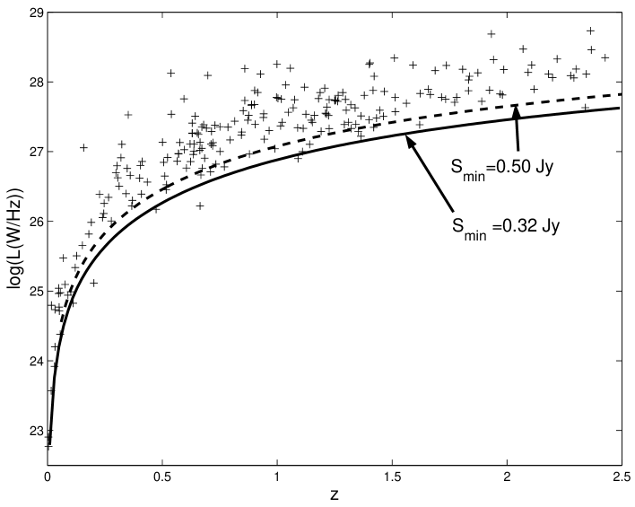
Figure 3: The luminosity and redshift sample (MOJAVE survey). The solid and dashed lines are the flux limit corresponding to 0.32 Jy and 0.50 Jy, respectively. For completeness, only the sources with $z<2.5$ are included.

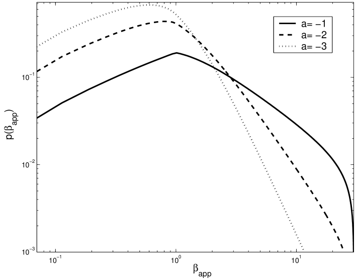
Figure 6: The pdf of the apparent velocity distribution with $p(\gamma)\propto\gamma^{a}(1<\gamma<30)$ and $n=2$. Three cases are shown, i.e. $a=-1$ (solid line), $a=-2$ (dashed line) and $a=-3$ (dot line).

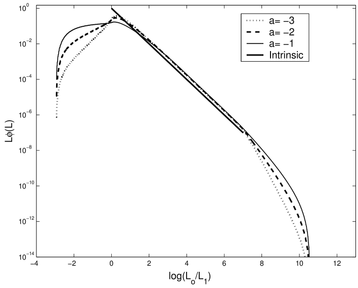
Figure 7: The observed luminosity function with $p(\gamma)\propto\gamma^{a}(1<\gamma<30)$ and $n=2$. The thick solid line is the intrinsic luminosity function, i.e. $\phi(L)\propto\L^{-2}\;(L_{1}<L<10^{7}L_{1})$. Three cases are shown, i.e. $a=-1$ (thin solid line), $a=-2$ (dashed line) and $a=-3$ (dot line).

References

- Author (2001) Arshakian, T. G. 2005, A&A, 436, 817
- Author (2001) Cohen, M. H., et al. 2007, ApJ, 658, 232
- Author (2001) Jackson, C. A., & Wall, J. V. 1999, MNRAS, 304, 160
- Author (2001) Kellermann, K. I., et al. 2004, ApJ, 609, 539
- Author (2001) Lister, M. L., & Marscher, A. P. 1997, ApJ, 476, 572
- Author (2001) Lister, M. L. 2003, ApJ, 599, 105
- Author (2001) Vermeulen, R. C., & Cohen, M. H. 1994, ApJ, 430, 467
- Author (2001) Padovani, P., & Urry, C. M. 1990, ApJ, 356, 75
- Author (2001) Padovani, P., & Urry, C. M. 1991, ApJ, 368, 373
- Author (2001) Padovani, P., & Urry, C. M. 1992, ApJ, 387, 449
- Author (2001) Urry, C. M., & Padovani, P. 1995, PASP, 107, 803
- Author (2001) Urry, C. M., et al. 1991, ApJ, 382, 501
- Author (2001) Willott, C. J., Rawlings, S., Blundell, K. M., & Lacy, M. 2000, MNRAS, 316, 449