Decorrelation of samples in Quantum Monte Carlo calculations and scaling of autocorrelation time in Li and H₂O clusters

Abstract

We have investigated decorrelation of samples in Quantum Monte Carlo (QMC) ground-state energy calculations for large Li and H₂O nanoclusters. Binning data as a way of eliminating statistical correlations, as is the common practice, is found to become increasingly impractical as the system size grows. We demonstrate nevertheless that it is possible to perform accurate energy calculations$-$without decorrelating samples$-$by exploiting the scaling of the integrated autocorrelation time $\tau$ as a function of the number of electrons in the system.

Quantum Monte Carlo (QMC) methods are becoming increasingly important in electronic structure calculations for a variety of systems of current interest review ; review2 . Although effective QMC methods have been developed in recent years to optimize the parameters of many-body wavefunctions umrigar88 ; sga ; rappe ; bressanini ; sorella ; filippi , QMC calculations are fundamentally limited by the statistical accuracy that can be obtained in a reasonable amount of computation time. Despite the growing maturity of core QMC techniques in terms of efficiency umrigar93b ; umrigar93 , computations of large clusters are hampered by increasing correlations in samples with increasing system size. In this connection, scaling of the computation time required to obtain a given statistical accuracy has been reported as a function of the atomic number $Z$ ceperley ; hammond ; ma , and also as a function of the number of atoms $M$ in non-metallic clusters galli . Here we discuss the effects of correlated sampling in Li and H₂O clusters.

When the number of atoms in a metallic cluster increases, the gap to the excited states shrinks as the electronic states begin to form a band and approach the bulk metallic character. This shrinking gap between the ground state and the excited states induces progressively greater statistical correlations among samples due to the Markovian character of the QMC sampling algorithm footnoteCorrelations . We address this problem through an analysis of the integrated autocorrelation time $\tau$ liu  which has not been considered in previous work on scaling; in particular, Williamson, et al. galli do not consider this correlation factor in their studies of non-metallic clusters. We demonstrate with the example of Li clusters that the problem of correlations among samples increases rapidly as the system size grows, making it increasingly difficult to decorrelate samples and determine the statistical error of the QMC calculation. Nevertheless, by invoking the scaling relationship of $\tau$, efficient computations of large clusters become feasible, even in the presence of highly correlated samples.

The relevant technical details of our calculations are as follows. For a given many-body wave function, $\Phi_{0}(x)$, we employ Umrigar’s modified version of discrete Langevin dynamics umrigar93 to generate a sequence of QMC samples footnote3 . Our QMC runs were carried out using a modification of the QMcBeaver code qmcbeaver . We chose to move all electrons during each QMC step rather than performing single-electron moves footnoteSingleGlobalExplanation . In all cases, an acceptance ratio of 50% was maintained. We note that achieving equilibration for large clusters is quite demanding. In particular, the Li₆₄ and $\left(\text{H}_{2}\text{O}\right)_{20}$ clusters each required about one week to equilibrate footnoteEquilibration .

After equilibration, the QMC walker’s steps follow a probability distribution $\pi(x)=|\Phi_{0}(x)|^{2}$. The estimate of the total energy $E$=$<\Phi_{0}|H|\Phi_{0}>$ is obtained from the average of the local energies $h(x)=H\Phi_{0}(x)/\Phi_{0}(x)$ over the steps taken by the walker. Estimates of $E$ from multiple independent calculations are distributed according to a normal distribution, with variance $\sigma^{2}$ estimated by liu

$$\sigma^{2}\approx\sigma_{0}^{2}(1+2\sum_{i=1}^{\infty}C_{h}(i)),$$ (1)

where $\sigma_{0}^{2}$ is the estimate of the variance of $E$ calculated as though the samples were uncorrelated, i.e. $\sigma_{0}^{2}=\sigma_{raw}^{2}/N$, where $\sigma_{raw}^{2}$ is the variance of $h(x)$ over $N$ steps. $C_{h}(i)$, the autocorrelation of $h$ at $i$ steps, is given by $C_{h}\left(i\right)=\left\langle h\left(x^{j}\right)h\left(x^{j+i}\right)\right\rangle-\left\langle h\left(x^{j}\right)\right\rangle^{2}$ (normalized to the point $i=0$), where $j$ is an arbitrary step number in the post-equilibration phase, and the brackets $\left\langle\ldots\right\rangle$ denote the expectation value over an infinite ensemble. The ”integrated autocorrelation time” $\tau$ is then defined such that the variance

$$\sigma^{2}=\sigma_{raw}^{2}/(N/\tau)\text{,}$$ (2)

so that the ”effective” number of steps taken by the walker is given not by $N$, but by $N/\tau$. Eq. 2 generalizes the statistical error whose scaling with system size has been discussed by Williamson, et al. galli by the addition of the quantity $\tau$, the factor which describes the effect of statistical correlations between QMC moves. In the discrete case at hand, we have

$$\tau=(1+2\sum_{i=1}^{\infty}C_{h}(i))~{}.$$ (3)

By comparing Eqs. (1) and (3), we see that

$$\tau=(\sigma/\sigma_{0})^{2}.$$ (4)

The ratio in Eq. 4 is sometimes also called the ”statistical inefficiency”; see Refs. FC ; KB ; AT . In order to determine the ratio $(\sigma/\sigma_{0})^{2}$ and thus obtain $\tau$, we employed the recently developed Dynamic Distributable Decorrelation Algorithm (DDDA) kent to block data efficiently. Like other data blocking algorithms footnote5 , the DDDA is a renormalization group method that relies on the appearance of a plateau to determine the correct variance of the mean value of the energy. The DDDA performs the blocking with nearly zero overhead both in time and in memory, and for these reasons it is well-suited for our study of the convergence properties of large systems.

Simulations were carried out on Li clusters with 4, 8, 20, 26 and 64 atoms lithium . Li is an interesting element because it displays subtle bonding properties MarxLi ; marx . Moreover, it contains only a few electrons per atom, which makes it possible to consider relatively large Li clusters. We have used Hartree-Fock footnoteHF  many-body wave functions $\Phi_{0}(x)$ constructed with one-particle orbitals obtained with the software Jaguar jaguar .

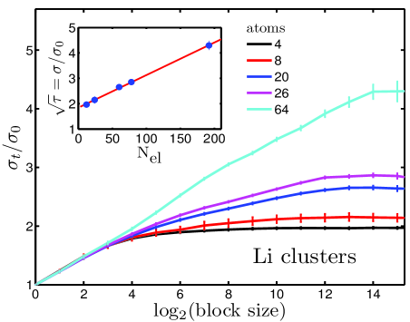
Figure 1: (Color online) Normalized trial standard deviation $\sigma_{t}/\sigma_{0}$ and its error bar for 4 to 64 atom Li clusters. Samples are decorrelated when $\sigma_{t}/\sigma_{0}$ displays a plateau, where the height of the plateau is related from Eq. 4 to the square root of the integrated correlation time, i.e. $\sqrt{\tau}=\sigma/\sigma_{0}$. Inset shows the linear scaling of $\sqrt{\tau}$ with the number of electrons $N_{el}$ in the system. Error bars on data points are comparable to dot sizes.

Fig. 1 shows the value $\sigma_{t}/\sigma_{0}$ plotted as a function of block size for Li clusters varying in size from 4-64 atoms, where $\sigma_{t}$ is the trial standard deviation at various block sizes in the computation. The horizontal axis gives the number of adjacent QMC samples (block size) pulled piecewise from the full set of samples and aggregated, creating effective samples which are used in the calculation of $\sigma_{t}$. The appearance of a plateau, or flat region, in the $\sigma_{t}/\sigma_{0}$ plot indicates full decorrelation of samples. The height of this plateau yields the true value of the normalized standard deviation $\sigma/\sigma_{0}$, which from Eq. 4 gives the correct value of the square root of the integrated correlation time, $\sqrt{\tau}$. For example, for the 4 atom cluster with $N_{e}$=12 electrons, the $\sigma_{t}/\sigma_{0}$ curve (black line) flattens to a value of about 2, which is the value shown for $\sqrt{\tau}$ in the inset. Similarly, the plateau for 20 Li atoms with 60 electrons (deep blue line) appears for $\sigma_{t}/\sigma_{0}$=2.7.

An increase in the height of the plateau, i.e., in the value of $\sigma/\sigma_{0}$ or equivalently of $\sqrt{\tau}$, with cluster size is evident in Fig. 1. More quantitatively, the inset reveals a linear relationship of $\sigma/\sigma_{0}$ with the number of electrons $N_{el}$ in the cluster. It thus follows that the autocorrelation time diverges quadratically with system size. We emphasize that the total number of points $n_{p}$ needed to reach the plateau for a given cluster size is much larger than the corresponding value of $\tau$. For example, for the 64 atom cluster the plateau appears in Fig. 1 at the value 14 or equivalently for $n_{p}=2^{14}$, while $\tau=(4.3)^{2}=18.5$. In other words, one would need to skip $2^{14}$ steps in this case if one wanted to decorrelate samples. Note that $\tau$ is an integrated correlation time; therefore, skipping $\tau$ steps will not produce decorrelated samples. Clearly, because $n_{p}$ grows so large, calculation of the error using reblocking rapidly becomes intractable for large clusters.

The total time of a computation can be written as $T=t_{s}N$, where $t_{s}$ is the time per step and $N$ is the total number of steps. From Eq. 2, we see that in order to maintain a given accuracy $\sigma$ for QMC calculations of different clusters, the number of steps $N$ must change to balance changes in $\sigma_{raw}^{2}$ and $\tau$. For quadratically scaling $\tau$, the number of steps $N$, and therefore the total computation time, will have an additional scaling factor of up to $M^{2}$, where $M$ denotes the number of atoms in the cluster, in order to compensate for the scaling of $\tau$. This additional scaling factor for $\tau$ is present whether the quantity being calculated is the energy for the entire system, or the energy per atom. The scaling factors due to $\sigma_{raw}^{2}$ and $t_{s}$ have been considered in previous work galli and are not considered in this study.

A QMC calculation is complete only when accompanied by a measure $\sigma$ of its statistical uncertainty, which is given by the onset of the decorrelation plateau in a plot such as that of Fig. 1. The failure to obtain this onset indicates that it is impossible to decorrelate samples during the run. This ”stickiness” of correlated samples in QMC runs impedes our ability to determine the statistical error $\sigma$ of the computation. Often, in order to decorrelate samples, the problem of stickiness is overcome by obtaining a large number of sample points and discarding intermediate correlated points. However, as we have already pointed out above, it becomes increasingly difficult in large clusters to obtain the plateau and decorrelate samples. It may in fact be impossible to decorrelate even a single sample during the run. In sharp contrast, our procedure requires that all steps are sampled, with no steps discarded, in order to first calculate $\sigma_{0}^{2}$, and then obtain $\sigma^{2}$ by rescaling with an extrapolated value of $\tau$. In this way, our scheme provides a route for circumventing the problem of decorrelating samples in large clusters.

As an example of an energy calculation obtained without observing the onset of a decorrelation plateau, we were able to obtain the energy (per atom) for the Li₆₄ cluster to within $\sigma=0.1$ eV ($\pm 10\%$) using only $10^{5}$ QMC steps footnoteHardware . We have verified our estimate of the accuracy of $\sigma$ for this energy calculation by performing multiple, independently equilibrated runs and observing the spread of the energy results.

We turn now to consider H₂O clusters, where we have studied clusters of 2, 4, 8, 9, 14 and 20 molecules water . These clusters have similar electron counts to those of the Li clusters discussed above. Fig. 2 shows decorrelation plots as a function of block size. All clusters display the onset of the decorrelation plateau. A comparison of the insets in Figs. 1 and 2 shows that the value of $\sqrt{\tau}=\sigma/\sigma_{0}$ varies significantly less rapidly with system size in H₂O clusters. It is striking that all curves in Fig. 2 collapse onto an essentially universal curve up to five block transformations. Beyond this block size, however, it appears that other secondary longer-distance correlations play a noticeable role so that the curves begin to rise again and settle into new, weakly size-dependent plateaux. If it were not for this secondary feature, all H₂O clusters would achieve their plateaux in the same small number of blocking steps, and the stickiness induced by correlated sampling would not be important. Because of these secondary features, H₂O clusters exhibit quadratic scaling of $\tau$ with $M$, but the influence is significantly less severe than for Li.  In fact, if $a+bN_{el}$ describes a linear fit for the data in the inset for H₂O, we see that for the cluster sizes we studied, the constant term in the quadratic expression $\tau=\left(\sqrt{\tau}\right)^{2}=\left(a+bN_{el}\right)^{2}$ dominates.  This may explain why the phenomenon was not observed in Ref. galli . For Li, the linear term dominates and adds to the scaling of the total computation time for the cluster sizes we studied.

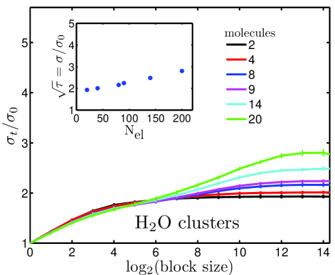
Figure 2: (Color online) Same as Fig. 1, except that this figure refers to H₂O clusters.

We now provide a possible explanation for the divergence of the autocorrelation time $\tau$ in ground state computations of Li clusters. We recall that bulk Li metal contains discontinuities in the momentum density of the electron gas at the Fermi momentum. Such a sharp cut-off in the momentum distribution can be expected to generally cause oscillations of electron configurations involved in the QMC algorithm and thereby slow the statistical convergence in clusters like those of Li atoms, which must eventually approach the bulk metallic state with increasing size. These considerations suggest that smearing or broadening the underlying ”Fermi surface” (formally, of course, there is no Fermi surface in a finite system) in metallic nanoclusters using a trial wavefunction such as an AGP agp or a Pfaffian pfaffian might result in shorter autocorrelation times. Notably, Baroni and Moroni baroni have discussed a theoretical connection between the autocorrelation time and the spectrum of an auxiliary quantum Hamiltonian, which might help explain the divergence of the autocorrelation time in metallic systems.

The integrated autocorrelation time $\tau$ is related to the second largest eigenvalue $\lambda$ of the transition matrix by $\tau=1+2\lambda/(1-\lambda)$ liu . Very recent work regarding the scaling of $\lambda$ in the Metropolis alorithm demonstrates that for log-concave distributions $|\Phi_{0}(x)|^{2}$, the scaling of $\tau$ with $M$ is at most $M^{2}$ novak . For Langevin dynamics the divergence of $\tau$ is usually less severe than in the Metropolis algorithm roberts . In principle, the appearance of nodes in the wavefunction can violate the log-concavity of $|\Phi_{0}(x)|^{2}$ and might modify the scaling properties of $\tau$. Although our wavefunctions contain nodes, the fact that we obtain a clear $M^{2}$ scaling of $\tau$ suggests that the $M^{2}$ scaling remains maximal for typical QMC distributions $|\Phi_{0}(x)|^{2}$ more generally footnotenodal .

In conclusion, we have investigated the scaling of the integrated autocorrelation time $\tau$ in QMC computations of Li and H₂O clusters. The quantity $\tau$, which directly yields a measure of sampling correlations in the calculation, is found to diverge quadratically with system size $M$ in both cases, more severely for Li than for H₂O, and becomes increasingly difficult to calculate for large clusters. We have shown that brute force decorrelation of samples is simply not feasible for these large clusters. Our study highlights the importance of correlated sampling in QMC computations of large clusters and provides a route for obtaining accurate error estimates by exploiting the scaling properties of $\tau$ with system size, without requiring explicit decorrelation of samples. The present results should be relevant for the growing scientific community liu interested in the convergence properties of Markov chains and QMC calculations of properties of nanoclusters. Further work towards understanding the effects of excitation gaps on the convergence of the QMC algorithm might be valuable.

We acknowledge useful discussions with Lubos Mitas, Chip Kent, Dario Bressanini, and Erich Novak, and we thank R. Rousseau and D. Marx for sending us atomic coordinates for Li clusters. This work was made possible by the support of the U.S.D.O.E. contracts DE-FG02-07ER46352 and DE-AC03-76SF00098. We benefited from the allocation of supercomputer time at NERSC and Northeastern University’s Advanced Scientific Computation Center (ASCC).

References

- (1) W. M. C. Foulkes, L. Mitas, R. J. Needs, and G. Rajagopal, Rev. Mod. Phys. 73, 33 (2001)
- (2) A. Luchow and J. B. Anderson, Ann. Rev. Phys. Chem. 51 501 2000
- (3) C. J. Umrigar, K. G. Wilson, and J. W. Wilkins, Phys. Rev. Lett. 60 1719 (1988)
- (4) A. Harju, B. Barbiellini, S. Siljamäki, R. M. Nieminen, and G. Ortiz, Phys. Rev. Lett. 79, 1173 (1997)
- (5) X. Lin, H. Zhang, and A. M. Rappe, J. Chem. Phys. 112, 2650 (2000)
- (6) D. Bressanini, G. Morosi, M. Mella, J. of Chem. Phys. 116, 5345 (2002)
- (7) S. Sorella, Phys. Rev. B 71, 241103(R) (2005); M. Casula and S. Sorella, J. Chem. Phys. 119, 6500 (2003)
- (8) C. J. Umrigar and C. Filippi, Phys. Rev. Lett. 94, 150201 (2005)
- (9) C. J. Umrigar, Phys. Rev. Lett. 71 408 (1993)
- (10) C. J. Umrigar, M. P. Nightingale and K. J. Runge, J. Chem. Phys. 99, 2865 (1993)
- (11) D. M. Ceperley, J. Stat. Phys. 43, 815 (1986)
- (12) B. L. Hammond, P. J. Reynolds, and W. A. J. Lester, Chem. Phys. 87, 1130 (1987)
- (13) A. Ma, N. D. Drummond, M. D. Towler, and R. J. Needs, Phys. Rev. E 71, 066704 (2005)
- (14) A. J. Williamson, R. Q. Hood, and J. C. Grossman, Phys. Rev. Lett. 87 246406 (2001)
- (15) The underlying algorithm of such simulations involves Markov chains liu . The data generated from a Markov chain are serially correlated, meaning that the covariance between data elements is nonzero (i.e., nearby points in the chain are also nearby in configuration space, not sampled uniformly from the desired distribution).
- (16) J. Liu, Monte Carlo Strategies in Scientific Computing, Springer-Verlag, New York (2001)
- (17) We use only one walker, because this is required for a study of the decorrelation plateau, defined later.
- (18) http://sourceforge.net/projects/qmcbeaver
- (19) We ran preliminary calculations of small Li clusters using single-electron moves. These calculations revealed similar modified autocorrelation times umrigar93b as global moves. Also, the QMC step size scales linearly with the inverse of the number of electrons for the Li clusters we studied, so that the total distance the electrons move remains the same, whether global or single-electron moves are used.
- (20) We performed a detailed study of Li64 and equilibration by running a massively parallel calculation (1024 processors), assuming the points were equilibrated (even when they were not), and noticing that the variational theorem demands that the energy be higher for unequilibrated systems. Therefore, only when the error bars for our massively parallel run overlapped the (known) HF energy did we consider our samples to be equilibrated.
- (21) R. Friedberg and J. E. Cameron, J. Chem. Phys. 52, 6049 (1970)
- (22) H. Muller-Krumbhaar and K. Binder, J. Stat. Phys. 8, 1 (1973)
- (23) M. P. Allen and D. J. Tildesley, Computer Simulations of Liquids, Oxford University Press, Oxford, 1987
- (24) D. R. Kent, ”New Quantum Monte Carlo Algorithms to Efficiently Utilize Massively Parallel Computers”, PhD Dissertation, California Institute of Technology (2003)
- (25) H. Flyvbjerg and H. G. Petersen, J. Chem. Phys. 91 , 461 (1989)
- (26) The geometry of Li clusters can be found in marx . For Li64 and Li26, we have extracted the geometry from bulk BCC Li.
- (27) R. Rousseau and D. Marx, Phys. Rev. Lett. 80 2574 (1998)
- (28) R. Rousseau and D. Marx, Chem. Eur. J. 6, 2982-2993 (2000)
- (29) The use of the HF wavefunction is adequate for our study, aimed at understanding convergence properties of QMC calculations, rather than obtaining an accurate value of the correlation energy. Also, by duplicating a known HF result, we can be certain the system is ergodic.
- (30) Jaguar 4.0, Schrödinger, Inc., Portland, OR
- (31) This run was performed on a Xeon EMT 64 3.0 GHz processor.
- (32) The geometry of H2O clusters can be found at http://www-wales.ch.cam.ac.uk/~wales/CCD/TIP4P-water.html
- (33) M. Casula, C. Attaccalite, and S. Sorella. J. Chem. Phys. 121, 7110 (2004)
- (34) M. Bajdich, L. Mitas, G. Drobny, L. K. Wagner, and K. E. Schmidt, Phys. Rev. Lett. 96, 130201 (2006)
- (35) S. Baroni, S. Moroni, in Quantum Simulations of Complex Many-Body Systems: From Theory to Algorithms, J. Grotendorst, D. Marx, A. Muramatsu (Eds.), John von Neumann Institute for Computing, Jülich, NIC Series, Vol. 10, p. 75 (2002)
- (36) P. Mathé and E. Novak, math.NA/0611285 (submitted to the Journal of Complexity)
- (37) G. O. Roberts and J. S. Rosenthal, Can. J. Stat. 26, 5 (1998).
- (38) The total energy is somewhat insensitive to the nodal structure of the wavefunction; see, e.g., G. F. Giuliani and G. Vignale, Quantum Theory of Electronic Liquids, Cambridge University Press, Cambridge (2005).