Weak-Light Ultraslow Vector Optical Solitons via Electromagnetically Induced Transparency

Abstract

We propose a scheme to generate temporal vector optical solitons in a lifetime broadened five-state atomic medium via electromagnetically induced transparency. We show that this scheme, which is fundamentally different from the passive one by using optical fibers, is capable of achieving distortion-free vector optical solitons with ultraslow propagating velocity under very weak drive conditions. We demonstrate both analytically and numerically that it is easy to realize Manakov temporal vector solitons by actively manipulating the dispersion and self- and cross-phase modulation effects of the system.

The vector nature of light propagating in a nonlinear medium has led to the discovery of a novel class of solitons, i. e. vector optical solitons, which are the solutions of two coupled nonlinear Schrödinger (NLS) equations describing the envelope evolution of two polarization components of an electromagnetic field. In recent years, considerable attention has been paid to the temporalmen ; isl ; bar ; cun ; kov ; ran and spatialseg ; kan ; ana ; del vector optical solitons in various nonlinear systems. Due to their remarkable property, vector optical solitons have promising applications for the design of new types of all-optical switches and logic gatesisl1 .

Up to now, most vector optical solitons are produced in passive media such as optical fibersisl ; bar ; cun ; kov ; ran ; seg ; kan ; ana ; del , in which far-off resonance excitation schemes are employed in order to avoid unmanageable optical attenuation and distortion. However, due to the lack of distinctive energy levels, the nonlinear effect in such passive media is very weak, and hence to form vector solitons a very high input light-power is required. In addition, the lack of distinctive energy levels and transition selection rules also makes an active control very difficult. In particular, it is hard to realize Manakovmanakov temporal vector optical solitons in optical fibers because the ratio between self-phase modulation (SPM) and cross-phase modulation (CPM) is not unity and there is also detrimental energy exchange between two polarization components due to the existence of four-wave mixing effect. Manakov vector optical solitons are of great interest, not only because the coupled NLS equations describing them have beautiful mathematical properties but also such solitons may be used to realize all-optical computingstei . Different from spatial Manakov vector optical solitons, which have been observed more than ten years agokan , temporal Manakov vector optical solitons have not been realized in experiment up to now.

In this Letter, we propose a scheme to generate temporal vector optical solitons in a coherent five-level atomic system via electromagnetically induced transparency (EIT). This resonant EIT medium has been recently used to realize polarization qubit phase gateott and reversible memory devices for photon-polarization qubitpet . We show that two continuous-wave (CW) control laser fields established prior to the injection of a pulsed probe field induce a quantum interference effect, which can suppress largely the absorption of the two orthogonal polarization components of the probe field. The scheme suggested here is fundamentally different from the passive ones due to the existence of distinctive energy-levels that make an active manipulation on the dispersion and nonlinear effects of the system possible. In addition, contrary to all passive schemes the vector optical solitons produced in the present system may have ultraslow propagating velocity and their production needs only very weak input power. Furthermore, the controllability of the present scheme allows us also to realize easily temporal Manakov vector optical solitons by actively adjusting the parameters of the system. Notice that scalar ultraslow optical solitons in EIT media have been investigated recentlywu ; huang ; hang . However, up to now there has been no study on the ultraslow vector optical solitons in an active optical medium. Our study represents the first work in this direction and the results may have potential application in optical information processing and engineering.

Consider a life-timed broadened five-level system (e. g. a Zeeman split atomic gas) interacting with a weak, pulsed, linear-polarized probe field of central frequency $\omega_{p}/(2\pi)$ and two strong, linear-polarized CW control fields of frequencies $\omega_{c1}/(2\pi)$ and $\omega_{c2}/(2\pi)$, respectively. The two polarization components of the probe field drive respectively the transitions from $|3\rangle\leftrightarrow|2\rangle$ and $|3\rangle\leftrightarrow|4\rangle$, while the two control fields drive respectively the transitions from $|1\rangle\leftrightarrow|2\rangle$ and $|5\rangle\leftrightarrow|4\rangle$ (see Fig. 1(a)). The atoms are trapped in a cell with the temperature lowed to $0.5\,\,\mu$K to cancel Doppler broadening and collisions. A possible arrangement of experimental apparatus is shown in Fig. 1(b).

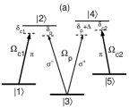
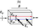
Figure 1: (a): Energy level diagram and excitation scheme of a five-level atomic system interacting with a weak, pulsed probe field of Rabi frequency $\Omega_{p}$ and two strong, CW coupling fields of Rabi frequency $\Omega_{c1}$ and $\Omega_{c2}$, respectively. (b): Possible arrangement of experimental apparatus.

The electric-field of the system can be written as ${\bf E}$=$({\bf\hat{\epsilon}}_{+}{\cal E}_{p+}+{\bf\hat{\epsilon}}_{-}{\cal E}_{p-})\exp[i(k_{p}z-\omega_{p}t)]+{\bf\hat{e}}_{c1}{\cal E}_{c1}\exp[i(k_{c1}y-\omega_{c1}t)]+{\bf\hat{e}}_{c2}{\cal E}_{c2}\exp[i(k_{c2}y-\omega_{c2}t)]+{\rm c}.{\rm c.}$. Here ${\bf\hat{\epsilon}}_{+}$=$({\bf\hat{x}}+i{\bf\hat{y}})/\sqrt{2}$  (${\bf\hat{\epsilon}}_{-}$=$({\bf\hat{x}}-i{\bf\hat{y}})/\sqrt{2}$) is the probe-field unit vector of the $\sigma^{+}$ ($\sigma^{-}$) circular polarization component with the envelope ${\cal E}_{p+}$ (${\cal E}_{p-})$, which drives the transition $|2\rangle\leftrightarrow|3\rangle$ ($|3\rangle\leftrightarrow|4\rangle$). ${\bf\hat{e}}_{c1}$  (${\bf\hat{e}}_{c2}$) is the unit vector of the control field with the amplitude ${\bf E}_{c1}$ (${\bf E}_{c2}$), which drives the transition $|1\rangle\leftrightarrow|2\rangle$ ($|4\rangle\leftrightarrow|5\rangle$). Thus the system is composed of two EIT $\Lambda$-configurations, both of them share the ground-state level $|3\rangle$ott ; pet .

In interaction picture, the atomic response of the system under rotating-wave approximation is described by

$$\left(\frac{\partial}{\partial t}+id_{1}\right)A_{1}=-i\Omega_{c1}^{\ast}A_{2},$$ (1a)

$$\left(\frac{\partial}{\partial t}+id_{2n}\right)A_{2n}=-i\Omega_{cn}A_{4n-3}-i\Omega_{pn}A_{3},$$ (1b)

$$\left(\frac{\partial}{\partial t}+id_{5}\right)A_{5}=-i\Omega_{c2}^{\ast}A_{4},$$ (1c)

($n$=$1,2$) with $\sum_{j=1}^{5}|A_{j}|^{2}$=$1$, where $A_{j}$ is the probability amplitude of the bare atomic state $|j\rangle$ (with eigenenergy $\epsilon_{j}$), $\Omega_{p1}$=$-(\textbf{p}_{23}$$\cdot$${\bf\hat{\epsilon}}_{-}){\cal E}_{p-}/\hbar$, $\Omega_{p2}$=$-(\textbf{p}_{43}$$\cdot$${\bf\hat{\epsilon}}_{+}){\cal E}_{p+}/\hbar$, $\Omega_{c1}$=$-(\textbf{p}_{21}$$\cdot$${\bf\hat{e}}_{c1}){\cal E}_{c1}/\hbar$ and $\Omega_{c2}$=$-(\textbf{p}_{45}$$\cdot$${\bf\hat{e}}_{c2}){\cal E}_{c2}/\hbar$ are half Rabi frequencies with $\textbf{p}_{ij}$ being the electric dipole matrix element associated with the transition from $|j\rangle$ and $|i\rangle$. In Eq. (1) we have defined $d_{1}=(\delta_{p}-\delta_{c1})-i\Gamma_{1}/2$, $d_{2}=\delta_{p}-i\Gamma_{2}/2$, $d_{3}=-i\Gamma_{3}/2$, $d_{4}=(\delta_{p}+\Delta)-i\Gamma_{4}/2$ and $d_{5}=(\delta_{p}+\Delta-\delta_{c2})-i\Gamma_{5}/2$ with $\delta_{p}=(\epsilon_{2}-\epsilon_{3})/\hbar-\omega_{p}$, $\delta_{c1}=(\epsilon_{2}-\epsilon_{1})/\hbar-\omega_{c1}$, and $\delta_{c2}=(\epsilon_{4}-\epsilon_{5})/\hbar-\omega_{c2}$. $\Gamma_{j}$ is the decay rate of the state $|j\rangle$, $\Delta=(2\mu_{B}/\hbar)gB$ is the Zeeman shift of the upper atomic sublevel with $\mu_{B}$ the Bohr magneton, $g$ the gyromagnetic factor and $B$ the applied magnetic field.

The equation of motion for $\Omega_{pn}(z,t)$ can be obtained by Maxwell equation under slowly-varying envelope approximation

$$i\left(\frac{\partial}{\partial z}+\frac{1}{c}\frac{\partial}{\partial t}\right)\Omega_{pn}-\kappa_{3l}A_{2n}A_{3}^{\ast}=0,\,\,\,\,(l=2n)$$ (2)

where $\kappa_{32}={\cal N}_{a}|\textbf{p}_{32}\cdot{\bf\hat{\epsilon}}_{-}|^{2}\omega_{p}/(2\hbar\epsilon_{0}c)$ and $\kappa_{34}={\cal N}_{a}|\textbf{p}_{34}\cdot{\bf\hat{\epsilon}}_{+}|^{2}\omega_{p}/(2\hbar\epsilon_{0}c)$ with ${\cal N}_{a}$ being the atomic density, $\epsilon_{0}$ the vacuum dielectric constant and $c$ the light speed in vacuum.

Before solving Eqs. (1) and (2), we examine the linear properties of the system, which provide main contributors to pulsed spreading and attenuation. We assume that the probe field is weak so that the atomic ground state $|3\rangle$ is not depleted, i.e., $A_{3}\approx$1. Taking $\Omega_{pn}$ and $A_{j}$ ($j=1,2,4,5$) as being proportional to $\exp[i(k(\omega)z-\omega t)]$, one can get two branches of linear dispersion relation $k_{1}(\omega)$=${\omega}/{c}+\kappa_{32}(\omega-d_{1})/{D_{1}(\omega)}$ and $k_{2}(\omega)$=${\omega}/{c}+\kappa_{34}(\omega-d_{5})/{D_{2}(\omega)}$, corresponding to $\sigma^{-}$ and $\sigma^{+}$ components of the probe field, respectively. Here we have defined $D_{1}(\omega)$=$|\Omega_{c1}|^{2}-(\omega-d_{1})(\omega-d_{2})$ and $D_{2}(\omega)$=$|\Omega_{c2}|^{2}-(\omega-d_{4})(\omega-d_{5})$.

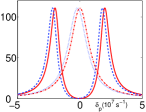
Figure 2: Absorption spectra of $\Omega_{p1}$ (solid line) and $\Omega_{p2}$ (dashed line) with parameters $\Gamma_{2}\simeq\Gamma_{4}=2\pi\times 6$ MHz, $\Gamma_{1}\simeq\Gamma_{3}\simeq\Gamma_{5}=2$ kHz, $\kappa_{32}\simeq\kappa_{34}=1.0\times 10^{9}$ cm^-1s^-1, $\Omega_{c1}=\Omega_{c2}=2.0\times 10^{7}$ s^-1, and $\delta_{c1}=\delta_{c2}=0$, and $\Delta=2.0\times 10^{6}$ s^-1. The dash-dotted (dotted) line represents the absorption spectra of $\Omega_{p1}$ ($\Omega_{p2}$) when the control fields are switched off.

Shown in Fig. 2(a) is the absorption spectra of $\Omega_{p1}$ and $\Omega_{p2}$. We see that near the central frequency of the probe field (i. e. at $\omega$=$0$), both Im($k_{1}$) and Im($k_{2}$) are close to zero, which means the absorption is greatly suppressed. The reason of such suppression of the probe field is due to the introduction of the two strong control fields that induce a quantum interference effect and thus make the two polarization components of the probe field transparent.

Because of the existence of dispersion effect, the probe field will distort during propagation. In the following we show that the SPM and CPM effects of the system may balance the dispersion. To this aim we apply the method of multiple-scaleshuang ; hang to investigate the weak nonlinear evolution of the probe field. We make the asymptotic expansion $A_{j}$=$\sum^{\infty}_{l=0}\mu^{l}A_{j}^{(l)}$ and $\Omega_{pn}$=$\sum^{\infty}_{l=1}\mu^{l}\Omega_{pn}^{(l)}$ with $A^{(0)}_{3}$=$1$ and $A^{(0)}_{j}$=0 ($j$=1,2,4,5), where $\mu$ is a small parameter characterizing the small population depletion of the ground state and all quantities on the right hand side of the asymptotic expansion are considered as functions of the multi-scale variables $z_{l}$=$\mu^{l}z$ and $t_{l}$=$\mu^{l}t$.

The leading order solution is given by $\Omega_{pn}^{(1)}=F_{n}\,\exp\{i[k_{n}(\omega)z_{0}-\omega t_{0})]\}$ with $F_{n}$ being yet to be determined envelope functions. At the second order, a solvability requires $i[\partial F_{n}/\partial t_{1}+V_{gn}\partial F_{n}/\partial z_{1}]=0$, where $V_{gn}$=$1/K_{1n}$ with $K_{11}=1/c+\kappa_{32}(|\Omega_{c1}|^{2}+d_{1}^{2})/(|\Omega_{c1}|^{2}-d_{1}d_{2})^{2}$ and $K_{12}=1/c+\kappa_{34}(|\Omega_{c2}|^{2}+d_{5}^{2})/(|\Omega_{c2}|^{2}-d_{4}d_{5})^{2}$. The solvability condition at the third order yields two coupled NLS equations

$$i\frac{\partial F_{n}}{\partial z_{2}}-\frac{K_{2n}}{2}\frac{\partial^{2}F_{n}}{\partial t_{1}^{2}}-(W_{nn}|F_{n}|^{2}+W_{nm}|F_{m}|^{2})e^{-2\bar{\alpha}_{n}z_{2}}F_{n}=0,$$ (3)

($m,n$=1, 2; $m\neq n$) where

$$K_{2n}=-2\kappa_{3l}\frac{d_{2n}|\Omega_{cn}|^{2}+2d_{4n-3}|\Omega_{cn}|^{2}+d_{4n-3}^{3}}{(|\Omega_{cn}|^{2}-d_{2n}d_{4n-3})^{3}},$$

$$W_{nn^{\prime}}=-\frac{\kappa_{3l}d_{4n-3}(|d_{4n^{\prime}-3}|^{2}+|\Omega_{cn^{\prime}}|^{2})}{D_{n}|D_{n^{\prime}}|^{2}},$$

($n,n^{\prime}$=1, 2) are the coefficients characterizing the dispersion ($K_{2n}$), SPM ($W_{nn}$) and CPM ($W_{nm}$, $n\neq m$) of the two polarization components of the probe field, respectively. $\bar{\alpha}_{n}=\mu^{2}\alpha_{n}$ with $\alpha=\text{Im}[K_{0n}]$ [$K_{0n}$=$k_{n}(0)$]. When returning to original variables and introducing $\delta$=$(1/V_{g1}-1/V_{g2})/2$, $V_{g}$=$2V_{g1}V_{g2}/(V_{g1}+V_{g2})$, and $\tau=t-z/V_{g}$, Eq. (3) can be written as the dimensionless form

$$i\left(\frac{\partial}{\partial s}+g_{An}\right)u_{n}+(-1)^{n-1}ig_{\delta}\frac{\partial u_{n}}{\partial\sigma}-\frac{g_{Dn}}{2}\frac{\partial^{2}u_{n}}{\partial\sigma^{2}}$$

$$-(g_{nn}|u_{n}|^{2}+g_{nm}|u_{m}|^{2})u_{n}=0,$$ (4)

where $s$=$z/L_{D}$, $\sigma$=$\tau/\tau_{0}$, and $u_{n}$=$(\Omega_{pn}/U_{0})e^{-i\tilde{K}_{0n}z}$ ($\tilde{K}_{0n}$=Re[$K_{0n}$]), $g_{An}$=$\alpha_{n}L_{D}$, $g_{\delta}$=$\text{sign}(\delta)L_{D}/L_{\delta}$, $g_{D1}$= $K_{21}/|K_{22}|$, $g_{D2}$=$\text{sign}(K_{22})$ and $g_{nn^{\prime}}$=$W_{nn^{\prime}}/|W_{22}|$. Here we have defined $L_{D}$=$\tau_{0}^{2}/|K_{22}|$ (dispersion length), and $L_{\delta}$=$\tau_{0}/|\delta|$ (group velocity mismatch length). $\tau_{0}$ is typical pulse length of the probe field. In order to get soliton solutions we have assumed that typical nonlinear length $L_{NL}=1/(U_{0}^{2}|W_{22}|)$ is equal to the dispersion length $L_{D}$.

Because coupled NLS Eq. (4) has complex coefficients, generally a vector soliton does not exist. However, as we show below that practical parameters can be found based on the EIT effect and hence the imaginary part of the coefficients can be much smaller than the corresponding real part. This leads to a shape-preserving vector optical soliton solution that can propagate for an extended distance without significant deformation. The system admits bright-bright, bright-dark, and dark-dark vector soliton solutions through a balance between the dispersion and nonlinear effects. The bright-bright vector soliton solution reads $u_{n}={\cal V}_{n}\rm{sech}\sigma\exp[i({\cal P}_{n}\sigma+{\cal Q}_{n}s)]$ ($n=1,2$) if the parameters fulfill the condition $g_{22}g_{D1}=g_{12}g_{D2}$. Here we have defined ${\cal P}_{n}=(-1)^{n-1}g_{\delta}/g_{Dn}$, ${\cal Q}_{n}=-g_{\delta}^{2}/(2g_{Dn})-g_{Dn}/2$, and ${\cal V}_{2}=[(g_{D1}-g_{11}{\cal V}_{1}^{2})/g_{12}]^{1/2}$. A bright-dark vector soliton solution is given by $u_{1}={\cal V}_{1}\rm{sech}\sigma\exp[i({\cal P}_{1}\sigma+{\cal Q}_{1}s)]$, $u_{2}={\cal V}_{2}\tanh\sigma\exp[i({\cal P}_{2}\sigma+{\cal Q}_{2}s)]$, where ${\cal P}_{n}=(-1)^{n-1}g_{\delta}/g_{Dn}$, ${\cal Q}_{1}=-{\cal P}_{1}g_{\delta}-g_{D1}(1-{\cal P}_{1}^{2})/2-g_{12}{\cal V}_{2}^{2}$, ${\cal Q}_{2}={\cal P}_{2}g_{\delta}+g_{D2}{\cal P}_{2}^{2}/2-g_{22}{\cal V}_{2}^{2}$, and ${\cal V}_{2}=[(g_{11}{\cal V}_{1}^{2}-g_{D1})/g_{12}]^{1/2}$. Here ${\cal V}_{1}$ is a free parameter.

Now we show that a realistic atomic system can be found that allows the bright-bright vector optical soliton described above. We consider a cold alkali atomic vapor (e. g., rubidium or cesium atoms) with the decay rates $\Gamma_{2}\simeq\Gamma_{4}=0.5\times 10^{7}$ s^-1, and $\Gamma_{1}\simeq\Gamma_{3}\simeq\Gamma_{5}=1.0\times 10^{4}$ s^-1. We take $\kappa_{32}\simeq\kappa_{34}=1.0\times 10^{9}$ cm^-1s^-1 (${\cal N}_{a}\sim 10^{10}$ cm^-3), $\Omega_{c1}=\Omega_{c2}=1.6\times 10^{8}$ s^-1, $\delta_{p}=1.0\times 10^{8}$ s^-1, $\Delta=2.0\times 10^{6}$ s^-1, $\delta_{c1}=0$, and $\delta_{c2}=3.0\times 10^{6}$ s^-1. With the above parameters, we obtain $K_{01}=-6.41+0.10i$ cm^-1, $K_{02}=-6.38+0.10i$ cm^-1, $K_{11}=(14.62-0.47i)\times 10^{-8}$ cm^-1s, $K_{12}=(14.72-0.47i)\times 10^{-8}$ cm^-1s, $K_{21}=(-4.56+0.25i)\times 10^{-15}$ cm^-1s², $K_{22}=(-4.64+0.26i)\times 10^{-15}$ cm^-1s², $W_{11}=(-9.37+0.15i)\times 10^{-16}$ cm^-1s², $W_{12}=(-9.44+0.15i)\times 10^{-16}$ cm^-1s², $W_{21}=(-9.34+0.15i)\times 10^{-16}$ cm^-1s², and $W_{22}=(-9.40+0.15i)\times 10^{-16}$ cm^-1s². Notice that the imaginary parts of these quantities are much smaller than their relevant real parts. The physical reason for such small imaginary parts is due to quantum destructive interference induced by two CW control fields (i. e. EIT effect). We obtain $L_{\delta}=116.8$ cm and $L_{D}=0.8$ cm with $\tau_{0}=6.0\times 10^{-8}$ s and $U_{0}=3.7\times 10^{7}$ s^-1. The dimensionless coefficients read $g_{\delta}=0.007$, $g_{D1}=-0.98$, $g_{D2}=-1.0$, and $g_{11}\simeq g_{12}\simeq g_{21}\simeq g_{22}=-1.0$. The group velocities of the two polarization components are respectively given by Re$(V_{g1})=2.28\times 10^{-4}$ $c$ and Re$({V}_{g2})=2.26\times 10^{-4}$ $c$, which means that the two polarization components of the vector optical soliton propagate with nearly matched, ultraslow propagating velocities.

As we have stressed, different from the passive media such as optical fibersisl ; bar ; cun ; kov ; ran ; seg ; kan ; ana ; del the parameters of our present EIT medium can be actively manipulated. Consequently the coefficients of Eq. (4) can be easily adjusted to allow us to realize a Manakov system, which is a completely integrable and can be solved by inverse-scattering transformmanakov . In fact, with the parameters given above Eq. (4) can be written as a near Makakov system ($m,n$=1, 2; $m\neq n$)

$$i\frac{\partial u_{n}}{\partial s}+\frac{1}{2}\frac{\partial^{2}u_{n}}{\partial\sigma^{2}}+(|u_{n}|^{2}+|u_{m}|^{2})u_{n}=R_{n}(u_{n}),$$ (5)

with $R_{n}(u_{n})\simeq-0.08iu_{n}$ describing the linear absorption effect. We see that $R_{n}$ is indeed a small quantity which can be taken as perturbation. The vector soliton solution of Eq. (5) after neglecting $R_{n}$ is $u_{1}=\cos\theta\,\rm{sech}(\sigma)\exp(is/2)$ and $u_{2}=\sin\theta\,\rm{sech}(\sigma)\exp(is/2)$ with $\theta$ being a free parameter. Note that since the injected probe field is $\pi$ (i. e. linear) polarized, the two polarization components should have equal amplitude, i. e. $\theta=\pi/4$.

Shown in Fig. 3 is the evolution of the two polarization components of the probe field versus dimensionless time $t/\tau_{0}$ and distance $z/L_{D}$. The plots are obtained by numerically integrating Eq. (4) by using a split-step fast Fourier transform method and the bright-bright soliton solution given above as an initial condition. To demonstrate the balance between the dispersion and nonlinear effects, we change the probe field amplitude $U_{0}$ while keep other parameters the same as those given above. Fig. 3(a) shows the case when the dispersion is dominant over nonlinearity (i. e. $U_{0}\tau_{0}<\sqrt{|K_{22}/W_{22}|}$). We see that in this case both polarization components spread and attenuate seriously. Fig. 3(b) shows that case when $U_{0}\tau_{0}$=$\sqrt{|K_{22}/W_{22}|}$, i. e. there is a balance between the dispersion and nonlinearity. In this situation a shape-preserving propagation of vector optical soliton over long distance (z=3.2 cm) is achieved.

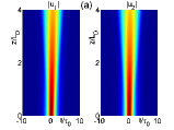
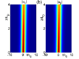
Figure 3: Evolution plots of the two polarization components of the probe field. (a): Dispersion dominant case with $U_{0}$=$3.7\times 10^{6}$ s^-1. (b): The case of a balance between dispersion and nonlinearity with $U_{0}$=$3.7\times 10^{7}$ s^-1. Brighter shading marks higher Rabi frequency. The propagation distance is $z=4L_{D}=3.2$ cm.

The input power of the vector optical soliton can be calculated by Poynting’s vector. It is easy to get the average flux of energy over carrier-wave period $\bar{P_{n}}$=$\bar{P_{n}}_{\rm{max}}\,\text{sech}^{2}[(t-z/V_{gn})/\tau_{0}]$, with the peak power $\bar{P_{1}}_{\rm{max}}\approx\bar{P_{2}}_{\rm{max}}=8.9\times 10^{-4}$ mW. Here we have taken $|\textbf{p}_{23}|\approx|\textbf{p}_{43}|=2.1\times 10^{-27}$ cm C and the beam radius of the probe laser $R_{\perp}=0.01$ cm. We see that to generate an ultraslow vector optical soliton in this active system only very low input power is needed. This is drastically different from the vector optical soliton generation schemes in passive midiaisl ; bar ; cun ; kov ; ran ; seg ; kan ; ana ; del where much higher input power is needed in order to bring out the nonlinear effect required for the soliton formation.

To make a further confirmation on the vector soliton solutions obtained and check their stability, we have made additional numerical simulation directly from Eq. (1) and (2) without using any approximations. Fig. 4 shows the simulation result by taking $u_{n}\,\,(z=0)=2\rm{sech}(2\sqrt{2}\sigma)$ ($n=1$, $2$) as initial condition. We see that the soliton radiates a small part of energy in its tail but is fairly stable during propagation.

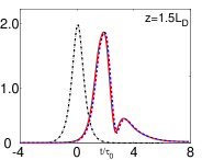
Figure 4: The bright-bright vector soliton evolution obtained by integrating directly from Eq. (1) and (2) without any approximations. The solid (dashed) line is for the $\sigma_{-}$ ($\sigma_{+}$) component of the relative probe intensity $|\Omega_{p1}/U_{0}|^{2}$ ($|\Omega_{p2}/U_{0}|^{2}$). The propagation distance is $z=1.5L_{D}=1.2$ cm.

In conclusion, we have proposed a scheme to create temporal vector optical solitons in a coherent five-level atomic system. Such solitons can have ultraslow propagating velocity and may be produced with extremely low input power. We have demonstrated both analytically and numerically that it is easy to realize Manakov temporal vector optical solitons by actively manipulating the dispersion and nonlinear effects of the system. Due to the robust propagation nature, the ultraslow vector optical solitons suggested here may have potential application in optical information processing and engineering under a weak-light level.

This work was supported by the NSF-China under Grant Nos. 90403008 and 10674060, and by the PhD Program Scholarship Fund of ECNU 2006.

References

(1)C. R. Menyuk, Opt. Lett. 12, 614(1987).
(2)M. N. Islam et al., Opt. Lett. 14, 1011(1989).
(3)Y. Barad and Y. Silberberg, Phys. Rev. Lett. 78,
3290(1997).
(4)S. T. Cundiff et al., Phys. Rev. Lett. 82,
3988(1999).
(5)A. E. Korolev et al., Opt. Lett. 30, 132(2005).
(6)D. Rand et al., Phys. Rev. Lett. 98,
053902(2007).
(7)M. Segev et al., Phys. Rev. Lett. 73, 3211(1994);
Z. Chen et al., Opt. Lett. 21, 1436(1996).
(8)J. U. Kang et al., Phys. Rev. Lett. 76, 3699(1996).
(9)C. Anastassiou et al., Opt. Lett. 26,
1498(2001).
(10)M. Delquè et al., Opt. Lett. 30,
3383(2005).
(11)S. V. Manakov, Sov. Phys. JETP 38, 248(1974).
(12)M. N. Islam, Ultrafast Fiber Switching Devices
and Systems (Cambridge Univ. Press, Cambridge, 1992).
(13)K. Steiglitz, Phys. Rev. E 63, 016608(2000).
(14)C. Ottaviani et al., Phys. Rev. Lett. 90, 197902(2003).
(15)D. Petrosyan, J. Opt. B: Quantum Semiclass. Opt. 7, S141(2005).
(16)Y. Wu and L. Deng, Phys. Rev. Lett. 93,
143904(2004).
(17)G. Huang et al., Phys. Rev. E 72,
016617(2005).
(18)C. Hang et al., Phys. Rev. E 73,
036607(2006).