Log-periodic drift oscillations in self-similar billiards

Abstract

We study a particle moving at unit speed in a self-similar Lorentz billiard channel; the latter consists of an infinite sequence of cells which are identical in shape but growing exponentially in size, from left to right. We present numerical computation of the drift term in this system and establish the logarithmic periodicity of the corrections to the average drift.

1 Introduction

Through the last decades, the theory of hyperbolic dynamical systems has become a cornerstone in the foundation of non-equilibrium statistical mechanics. The interest in hyperbolic models stems from relations between macroscopic features characteristic of irreversible phenomena, such as entropy production or transport coefficients, and dynamical properties, such as Lyapunov exponents [1, 2, 3, 4].

Billiard models, whose dynamics are conveniently described by the respective collision map, have proved extremely useful in this regard [5]. The simplest example is the two-dimensional periodic Lorentz gas with finite horizon, which exhibits diffusion without a drift [6]. In a statistically stationary state, this model represents a mechanical system at equilibrium, whose distribution, measured along the boundary of the scattering discs, is uniform in the position and normal velocity angles. Meanwhile the process of relaxation to equilibrium itself is characterized by deterministic hydrodynamic modes of diffusion with fractal properties [7]. One can also induce a non-equilibrium stationary state on a cylindrical version of this billiard by coupling it to stochastic reservoirs of point-particles at its boundaries [8]; these are the so-called flux boundary conditions. In this case, a difference between the chemical potentials of the reservoirs will transform to a linear gradient of density across the system, which is responsible for a steady current, given according to Fick’s law of diffusion, and positivity of the entropy production, see [3].

Whereas the previous examples of billiards are Hamiltonian systems which preserve the phase volume, one can also consider dissipative periodic billiards driven out of equilibrium by the action of an external field. Thus the Gaussian iso-kinetic periodic Lorentz gas is similar to the usual periodic Lorentz gas, but for the action of a thermostated uniform external field which bends the trajectories in the direction of the field while keeping the particle’s kinetic energy constant [1]. This field therefore induces a non-equilibrium stationary state to which is associated a constant drift current, according to Ohm’s law [9]. Moreover, due to the dissipation induced by the thermostat, phase-space volume is, on average, contracted. Therefore the sum of the Lyapunov exponents is strictly negative in the presence of the field and one can in fact identify this sum as minus the entropy production rate [10].

Gaussian iso-kinetic dynamics are different from Hamiltonian dynamics in that the latter preserve the total energy, whereas the former preserve the kinetic energy. One can nevertheless describe the Gaussian iso-kinetic dynamics by a Hamiltonian formalism, as shown in [11]. A general theorem due to Wojtkowski [12] stipulates that Gaussian iso-kinetic trajectories are geodesic lines of the so-called torsion free connection (also known as the Weyl connection). The Gaussian iso-kinetic Lorentz gas can thus be conformally transformed into a distorted billiard table on which trajectories become straight lines; besides, the conformal transformation preserves the specular character of the collision laws [13]. Although the trajectories thus transformed do not have constant speed anymore, one can introduce, for any given trajectory, a time-reparametrization under which the speed does remain constant.

A volume-preserving billiard in a distorted channel is therefore a natural generalization of iso-kinetic dynamics in a field-driven Lorentz channel. Ignoring the strict periodicity of the latter billiard, one may put aside the problem of time scales altogether and consider the dynamics of independent point-particles moving at constant speed in the new geometry. Such self-similar billiard channels were introduced in [14, 15]; they consist of an infinite sequence of (nonidentical) two-dimensional cells that are attached together and make a (nonuniform) one-dimensional channel. The cells are identical in shape, but their sizes are scaled by a common factor. As a particle moves from one cell to a neighbouring one, its velocity remains unchanged while the length scales are expanded (or contracted), so that the time scales between collisions change accordingly. A noticeable property of these billiards concern their long-term statistics; even though their dynamics preserve phase-space volumes, their statistics are characterized by a non-equilibrium stationary state with fractal properties and a drift, quite similar to the Gaussian iso-kinetic Lorentz gas itself. Close to equilibrium (when the scaling between neighbouring cells is close to unity), one can relate the constant drift velocity to the diffusion coefficient of the equilibrium system, which is none but the usual Lorentz channel, see [15].

In a recent paper [16], Chernov and Dolgopyat unveiled a remarkable feature of the drift term of self-similar billiards. Namely that the linear growth of the particle’s average displacement with respect to time is periodic on logarithmic time scales, or log-periodic, with a period specified by the scaling parameter. This term may therefore display periodic oscillations. The purpose of this paper is to provide further insight into this peculiar phenomenon, which actually stems from the discrete scale invariance of self-similar billiards [17]. We will offer numerical evidence which demonstrates the existence of log-periodic drift oscillations for self-similar billiards which are sufficiently far away from equilibrium. Closer to equilibrium, these oscillations are, at least numerically, found to vanish. Thus, for all practical purposes, we may assume the drift is constant close to equilibrium, and grows as a linear function of the scaling parameter. Further away from equilibrium, this linear dependence of the average drift in the scaling exponent remains valid, despite the presence of drift oscillations.

The paper is organized as follows. The model is described in section 2, which is a slight modification of the models previously studied in [14, 15]. Statistical properties of the model are briefly discussed in section 3. The characteristics of stationary drift, with numerical results, are presented in section 4. Conclusions and perspectives are offered in section 5.

2 Description of the model

In order to display the log-periodicity of the drift function of self-similar billiards discussed in section 4, which was predicted in [16], we will modify the self-similar billiard that was defined earlier in [14, 15], and use a unit cell rather similar to the one obtained after conformal transformation of the iso-kinetic Lorentz channel [13]. The resulting cell has enhanced symmetry in that all the discs are now equivalent. The main motivation for introducing this modification is that it allows to take much greater values of the scaling parameter within the constraints imposed to guarantee ergodicity.

In order to define the self-similar channel, we start with the description of the reference cell, examples of which are shown in figure 1.

Figure 1: Three examples of unit cells with short trajectories. The parameter values (defined in the text) are respectively $\epsilon=0.5$ and $\rho=0.459738$ (left), $\epsilon=1.$ and $\rho=0.440862$ (center), and $\epsilon=1.5$ and $\rho=0.413317$ (right).

We define the reference cell as the interior of a region bounded on the right and left sides by two arc-circles, with common center and respective radii $\exp(\pm\epsilon/2)/\epsilon$, and, on the upper and lower sides, by two oblique lines of slopes $\pm\tan\sqrt{3}\epsilon/2$, with the exclusion of obstacles, which are here taken to be regular discs. The parameter $\epsilon$ will henceforth be referred to as the scaling exponent, in contrast to the parameter $\mu$ which was defined in [14, 15] (or $r$ in [16]), and which we refer to as the scaling factor, $\mu=\exp(\epsilon)$.

Let the origin $(x,y)=(0,0)$ be on the middle of the arc-circle of the left-hand side border. We have the central disc of radius $\rho$, located at

$$(x,y)=\Big{(}\frac{1-\exp(-\epsilon/2)}{\epsilon},0\Big{)},$$

two discs of radii $\rho\exp(-\epsilon/2)$ on the inner circle, at

$$\Big{(}\frac{\exp(-\epsilon/2)}{\epsilon}[\cos(\sqrt{3}\epsilon/2)-1],\pm\frac{\exp(-\epsilon/2)}{\epsilon}\sin(\sqrt{3}\epsilon/2)\Big{)},$$

and two discs of radii $\rho\exp(\epsilon/2)$ on the outer circle, at

$$\Big{(}\frac{\exp(\epsilon/2)}{\epsilon}\cos(\sqrt{3}\epsilon/2)-\frac{\exp(-\epsilon/2)}{\epsilon},\pm\frac{\exp(\epsilon/2)}{\epsilon}\sin(\sqrt{3}\epsilon/2)\Big{)}.$$

Moreover, the corners where the boundaries of the cell intersect are located exactly at the centers of the outer discs.

Let $\mathcal{D}_{0}$ denote the reference cell. The extended system is obtained from the reference cell thus defined by making a copy of it, denoted by $\mathcal{D}_{1}$, which we scale by a factor of $\exp(\epsilon)$ and attach to the right-hand side of the reference cell. Likewise, another copy of the reference cell, this time denoted by $\mathcal{D}_{-1}$, is scaled by $\exp(-\epsilon)$ and attached to its left-hand side. By repeating this procedure, copying and scaling the right- and left-most cells and attaching these copies to the existing sequence of cells, we obtain the self-similar Lorentz channel, which consists of an infinite collection $\{\mathcal{D}_{n}\}_{n\in\mathbb{Z}}$ of such cells. Obviously the usual Lorentz channel [3] is recovered for $\epsilon=0$.

Note that when the value of $\rho$ is large enough with respect to $\epsilon$ , the central circle of the reference cell $\mathcal{D}_{0}$ will intersect with its inner arc-circle border. Correspondingly a sixth disc appears in the reference cell, whose center is located in cell $\mathcal{D}_{1}$, to the right of the reference cell (as is the case in the examples shown in figure 1). This happens when $\rho\geq[1-\exp(-\epsilon/2)]/\epsilon$.

A point-particle which moves in this extended system has unit speed and bounces off elastically when it collides with the scatterers and upper and lower walls. The circular walls which separate the cells from one another have no incidence on the dynamics.

As noticed in [14], the dynamics on the extended system can be boiled down to a single cell. Periodic boundary conditions, with rescaling of the arc-lengths and velocities, must then be imposed when trajectories collide on the circular sides to the right and left, reappearing on the opposite sides.

3 Ergodic properties

Although the geometry of the self-similar Lorentz channel is similar to that of the conformal transformation of the Gaussian iso-kinetic Lorentz gas, their dynamics are very different. By taking circular scatterers for all values of $\epsilon$, we ensure that no transition to a non-hyperbolic regime will occur. Nevertheless the similarities between the two lead to several immediate results regarding the ergodic properties of self-similar billiards. We refer the reader to [16] for more details.

Two constraints have to be imposed on the parameter values, which have straightforward expressions in this geometry.

The first constraint is the finite horizon condition, by which we avoid the possibility that some trajectories be ballistic. It is a straightforward generalization of the corresponding condition in the periodic Lorentz gas and here becomes

$$\rho>\rho_{\mathrm{min}}\equiv\frac{\sin(\sqrt{3}\epsilon/4)}{\epsilon}.$$ (1)

The second condition is that two discs on the same radius (with center at $\exp(-\epsilon/2)/\epsilon$) do not overlap so that the cell remains connected,

$$\rho<\rho_{\mathrm{max}}\equiv\frac{1}{\epsilon}\frac{\exp(\epsilon)-1}{\exp(\epsilon)+1}.$$ (2)

The parameter values compatible with these two conditions are shown in figure 2.

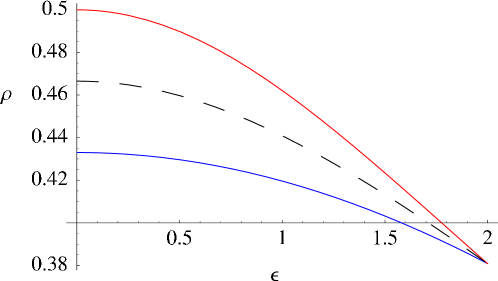
Figure 2: Allowed values of $\rho$ v. $\epsilon$ from equations (1) ($\rho$ above the blue curve), and (2) ($\rho$ below the red curve). Ergodicity will not be guaranteed outside the domain bounded by these two curves. The dashed line indicates the line of parameters we use in the computations presented in section 4.

4 Oscillations of the drift

Because of the biased geometry of the system, point-particles will preferentially move from small cells to large cells, i. e. from left to right, thus inducing a current of mass along the horizontal axis of the channel. Let $q(T)$ denote the displacement along this line after a time $T$. On average, $q(T)$ grows linearly in $T$, which is to say the current has a steady average value in time.

To be more precise, one can prove [16] that the ratio $q(T)/T$ remains of order one, in the sense that for any (small) $p>0$ there are constants $0<a<b<\infty$ such that $q(T)/T$ stays between $a$ and $b$ with probability $1-p$. However, a detailed analysis [16] shows the current may actually retain a time dependence between those bounds.

The reason is that the probability distribution of the ratio $q(T)/T$ does not stabilize as $T\to\infty$; rather it keeps oscillating. This happens because the cell sizes grow exponentially; thus the size of the current cell (that is the cell where the particle is located at time $T$) is comparable to its entire previous displacement $q(T)$. To emphasize this effect, assume for a moment that the scaling factor between neighboring cells is $2$ (i. e. the scaling exponent $\epsilon=\ln 2$). Then the current cell would be just as big as all the previous cells combined. In other words, the geometric shape of the current cell scales up at the same rate as the particle’s entire path.

This observation should convince the reader that the geometric structure of the current cell might affect the macroscopic evolution of $q(T)/T$. For example, there may be some parts of the cell which, on average, the particle traverses faster than others; in that case, as it passes through ‘fast terrain’, the ratio $q(T)/T$ would grow, and as it drags itself through ‘slow motion areas’, the ratio $q(T)/T$ would decrease. This happens periodically, as the particle moves from one cell to the next (even bigger) cell.

Note that the period of these oscillations is not fixed; it keeps growing exponentially with $T$. More precisely, the length of the period corresponds to the time it takes the particle to traverse the current cell completely, thus the ratio $\log q(T)/\epsilon$ should have period one.

These arguments were made precise in [16], where the following theorem was proved :

Theorem 1

Assume $\epsilon$ is chosen such that equations (1) and (2) are satisfied. The following holds. Let $\{T_{n}\}_{n\in\mathbb{N}}$ be a sequence of increasing times, $T_{n}\to\infty$, such that the fractional part of $\log T_{n}/\epsilon$ tends to a constant $0\leq\delta<1$. Then the distribution of $q(T_{n})/T_{n}$ converges to a limit.

The theorem also implies that the limit of $q(T_{n})/T_{n}$ may depend on the limiting fractional part of $\log T_{n}/\epsilon$, i. e. of $\delta$. We may therefore expect that $\langle q(T)\rangle/T$ will display oscillations as a function of $\log T/\epsilon$, with unit period. On the other hand, there may be no oscillations. Whether we can observe this oscillatory regime or not depends on the parameter values, as our numerical analysis reveals.

For the purpose of numerically demonstrating the drift oscillations, we let the scaling exponent $\epsilon$ to vary between $0$ and its maximal allowed value near $\epsilon=2$ (see figure 2) and take the corresponding radius to be $\rho=1/2(\rho_{\mathrm{max}}+\rho_{\mathrm{min}})$, in between the two bounds specified by equations (1) and (2). The precise values of the parameters we used in our computations are shown in Table 1.

Table 1: Parameter values used in the computations whose results are displayed in figures 3, 4 and 5.

$\epsilon$	$\rho$	$\epsilon$	$\rho$	$\epsilon$	$\rho$	$\epsilon$	$\rho$
0.1	0.466231	0.6	0.456839	1.1	0.435921	1.60000	0.407108
0.2	0.465406	0.7	0.453475	1.2	0.430665	1.70000	0.400732
0.3	0.464040	0.8	0.449670	1.3	0.425125	1.80000	0.394213
0.4	0.462145	0.9	0.445456	1.4	0.419333	1.90000	0.387575
0.5	0.459738	1.0	0.440862	1.5	0.413317	1.99765	0.380998

Figure 3 shows the results of numerical computations of the drift function $\langle q(T)\rangle/T$ using $10^{7}$ trajectories with random initial conditions located on the central circle (or on the discs on the horizontal line when there is an overlap) of cell $\mathcal{D}_{0}$, and unit velocity at random angle. For each of these trajectories, we computed the horizontal position $q(T)$ at times $T$ which we took to be logarithmically spaced on the interval $0\leq\log T/\epsilon\leq 100$, so as to have $25$ points on each unit interval of the scale $\log T/\epsilon$.

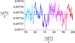
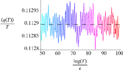
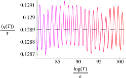
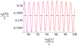
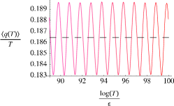
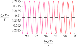
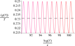
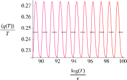
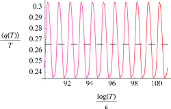
Figure 3: Average drift terms $\langle q(T)\rangle/T$ vs. $\log(T)/\epsilon$. Here shown are the parameter values of Table 1 corresponding to $\epsilon=0.8$, $0.9$, $1.0$, $1.2$, $1.4$, $1.6$, $1.8$, $1.9$ et $1.99765$, in order of increasing $\epsilon$, left to right and top to bottom. The dashed lines show the computed averages, as plotted in figure 5 below. The color code is a hue, regularly varying from cyan to red as units of $\log T/\epsilon$ increase from 50 to 100. Note that the span of the $x$-axis was reduced for the larger $\epsilon$ values in order to better display the periodicity of the oscillations.

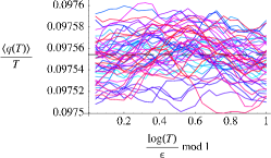
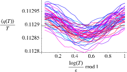
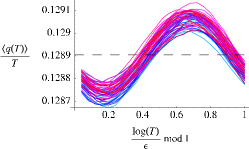
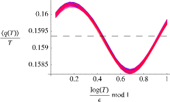
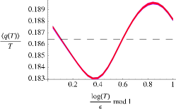
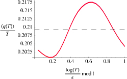
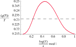
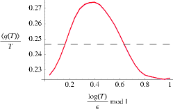
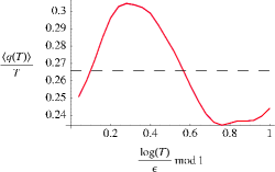
Figure 4: Same as figure 3 with the horizontal axis taken modulo 1. For every figure, we plot the last 50 oscillations. The color code is identical to figure 3. When $\epsilon$ is large enough, the curves nicely collapse on the same periodic function.

For values of the scaling exponent $\epsilon\geq 1.0$, the regularity of the observed periodic oscillations is spectacular, as confirmed by the collapsed curves of figure 4. On the contrary, for values of $\epsilon\leq 0.8$ (only $\epsilon=0.8$ is shown on figures 3 and 4), our measurements do not reveal periodic oscillations predicted by theorem 1, which, in principle, applies to all values of $\epsilon$. The lack of noticeable periodic oscillations for small $\epsilon$ is, most likely, the effect of insufficient time period $T$ in our simulation (recall that theorem 1 only holds asymptotically, as $T\to\infty$). It is (theoretically) possible that, after many more (say, $10^{3}$ or $10^{4}$) initial periods we would see proper periodic oscillations.

The summary of our computational results is shown in figure 5. The left-hand panel shows the average drift as a function of $\epsilon$, computed by taking the average of the time series of $\langle q(T)\rangle/T$ for every parameter value of Table 1. The right-hand panel shows the computed average amplitude of the oscillations, which we denote by $A$, with the corresponding error bars. The amplitudes of the oscillations is here measured by taking the average of one half of the sum of the maximum and minimum values of $\langle q(T)\rangle/T$ over each unit interval of $\log T/\epsilon$, which corresponds to a period of oscillation. Values of $\epsilon\leq 0.7$ were discarded, because oscillations could not be observed (yet).

Figure 5: Average drifts (left) and oscillation amplitudes (right) measured for the parameter values of table 1.

The latter graph clearly demonstrates a power law behavior of the amplitude in the scaling factor, i. e. $A\sim\exp(a\epsilon)$, with the coefficient $a\simeq 1.5$, for parameter values $1.5<\epsilon<2.0$. The coefficient seems to be somewhat larger for smaller values of $\epsilon$. The reason for this difference we believe is due to a non-trivial dependence in the parameter $\rho$, which here varies non-linearly with $\epsilon$. It might also be due to our limited statistics (as also reflected by the large error bars).

5 Concluding remarks

To conclude, self-similar billiard channels are instances of non-equilibrium chaotic billiards with volume-preserving dynamics, whereby a geometric constraint induces a current of mass, going from the smaller to the larger scales. The paper clearly establishes the following three novel results :

1. The average drift is a linear function in the scaling exponent $\epsilon$ throughout its range of allowed values.

2. When the scaling exponent is large enough, log-periodic drift oscillations do occur, i. e. the drift is not a constant.

3. The amplitude of the oscillations follows a power law in the scaling factor, more clearly so for the larger range of parameter values.

It is to be noted that property (ii) is an expected consequence of the discrete scale invariance of the system, which typically manifests itself in the presence of power laws with complex exponents. The signature of such power laws is the log-periodic corrections to their scalings, in this case the corrections to $q(T)\sim T$. Similar phenomena are observed in many different physical situations, see [17] and references therein. That the drift oscillations are barely noticeable when the scaling exponent decreases below $\epsilon=1.0$ is perhaps not surprising as log-periodicity is typically a very small effect. Going to the other end of the parameter range, it is actually remarkable that the regularity of drift oscillations is so well pronounced for larger values of $\epsilon$. In this regard, self-similar billiards offer new ground to further studies of this interesting phenomenon, here in the framework of hyperbolic dynamical systems, and thus improve our understanding of a ubiquitous property which has already found many known fields of applications.

References

References

- [1] Hoover W G 2001 Time Reversibility, Computer Simulation, and Chaos (World Scientific, Singapore).
- [2] Evans D J and Morriss G P 1990 Statistical Mechanics of Non-Equilibrium Fluids (Academic Press, London).
- [3] Gaspard P 1998 Chaos, Scattering and Statistical Mechanics (Cambridge University Press, Cambridge).
- [4] Dorfman J R 1999 An Introduction to Chaos in Nonequilibrium Statistical Mechanics (Cambridge University Press, Cambridge).
- [5] Chernov N I and Markarian R 2006 Chaotic billiards Math. Surveys and Monographs 127 (AMS, Providence, RI).
- [6] Bunimovich L A, Sinai Ya G, and Chernov N I 1991 Statistical properties of two-dimensional hyperbolic billiards Russ. Math. Surv. 46 47.
- [7] Gaspard P, Claus I, Gilbert T, and Dorfman J R 2001 The fractality of the hydrodynamic modes of diffusion Phys. Rev. Lett. 86 1506.
- [8] Gaspard P 1997 Chaos and hydrodynamics Physica A 240 54.
- [9] Chernov N I, Eyink G L, Lebowitz J L, and Sinai Ya G 1993 Derivation of Ohm’s law in a deterministic mechanical model Phys. Rev. Lett. 70 2209; 1993 Steady state electric conductivity in the periodic Lorentz gas Comm. Math. Phys. 154 569.
- [10] Ruelle D 1996 Positivity of entropy production in non-equilibrium statistical mechanics J. Stat. Phys. 85 1; 2003 Extending the definition of entropy to non-equilibrium steady states Proc. Nat. Acad. Sci. 100 30054.
- [11] Dettmann C P and Morriss G P 1996 Hamiltonian formulation of the Gaussian iso-kinetic thermostat Phys. Rev E 54 2495; Morriss G P and Dettmann C P 1998 Thermostats: analysis and application Chaos 8 321.
- [12] Wojtkowski M P 2000 W-flows on Weyl manifolds and Gaussian thermostats J. Math. Pures Appl. 79 953.
- [13] Barra F and Gilbert T 2007 Non-equilibrium Lorentz gas on a curved space J. Stat. Mech. 7 L01003.
- [14] Barra F, Gilbert T and Romo M 2006 Drift of particles in self-similar systems and its Liouvillian interpretation Phys. Rev. E 73 026211.
- [15] Barra F and Gilbert T 2007 Steady-state conduction in self-similar billiards Phys. Rev. Lett. 98 130601.
- [16] Chernov N and Dolgopyat D 2007 Particle’s drift in self-similar billiards preprint.
- [17] Sornette D 1998 Discrete scale invariance and complex dimensions Phys. Rep. 297 239.