The Nature of Linearly Polarized Millimeter and Sub-millimeter Emission in Sagittarius A*

Abstract

The linearly polarized millimeter and sub-millimeter emission in Sagittarius A* is produced within 10 Schwarzschild radii of the supermassive black hole at the Galactic Center and may originate from a hot magnetized accretion disk, where electrons are heated efficiently by turbulent plasma waves. In such a scenario, the flux density and polarization are very sensitive to the electron heating rate and the inclination angle of disk, respectively, and the major axis of the sub-millimeter intrinsic polarization, which is aligned with the rotation axis of the disk, is perpendicular to the major axis of the polarized near-infrared emission. In combination with MHD simulations, which study the properties of the magnetic field and viscous stresses, the current spectral and polarization measurements give tight constraints on the model parameters. Simultaneous observations will be able to test the model.

1 Introduction

Our understanding of physical processes in Sagittarius A*, the compact radio source associated with a supermassive [$M\simeq 3.7\times 10^{6}M_{\odot}$] black hole at the Galactic Center (Schödel et al. 2002; Ghez et al. 2005a), has improved dramatically since the detection of linear polarization of its millimeter and sub-millimeter emission (Aitken et al. 2000). It is generally accepted that Sagittarius A* is powered by accretion of the black hole in stellar winds (Melia 1992; Narayan 1998; Rockefeller et al. 2004). The linear polarization reveals a synchrotron origin of the emission and sets strict constraints on the magnetic field, gas density, and electron temperature (Agol 2000; Melia et al. 2000; Quataert & Gruzinov 2000). Recent VLBI imaging shows that the 3.5 mm emission is produced within $10\ r_{S}$ of the black hole, where $r_{S}\simeq 1.1\times 10^{12}[M/(3.7\times 10^{6}M_{\odot})]$ cm is the Schwarzschild radius for a non-spinning black hole (Shen et al. 2005). The emission may originate from a hot magnetized accretion disk, and simultaneous spectrum and polarization measurements can be used to estimate the model parameters (Bromley et al. 2001).

High spatial and spectral resolution X-ray and near-infrared (NIR) observations routinely detect flares from the direction of Sagittarius A* (Baganoff et al. 2001; Genzel et al. 2003). The characteristic variation time scale of a few tens of minutes, comparable to the dynamical time at the last stable orbit, indicates that they are also produced within a few $r_{S}$ of the black hole. The spectra, polarization, and variability, especially when considering results from simultaneous multi-wavelength observations, suggest that the NIR radiation is emitted through synchrotron processes and the X-rays are likely due to the synchrotron self-Comptonization (Eckart et al. 2006a, 2006b; Yusef-Zadeh et al. 2006a). The flares can be triggered by rapid releases of magnetic field energy near the black hole, which then heats electrons to a few tens of MeV producing the observed emission (Liu et al. 2004; Bittner et al. 2007). The long wavelength radio emission is less variable. The low quiescent-state X-ray flux and high centimeter radio flux density uncover a non-thermal origin of the emission and/or emission from an unbounded flow at large radii (Liu & Melia 2001; Yuan et al. 2002). Correlated flare activities in the X-ray and radio bands suggest that the radio emission is associated with an outflow (Zhao et al. 2004; Yusef-Zadeh et al. 2006b).

Recent SMA and BIMA observations confirm the linear polarization of the millimeter and sub-millimeter emission (Bower et al. 2005; Marrone et al. 2006a, 2006b). These observations not only show that the flux density and polarization are variable on time scales as short as a few hours but also reveal a relatively high mean flux density and hard spectrum in the sub-millimeter band as compared with the millimeter spectral bump first observed by Falcke et al. (1998). The observed position angle of the polarization vector has been used to infer an external Faraday rotation measure of $\sim-50$ rad cm^-2 (Macquart et al. 2006; Marrone et al. 2007) and a position angle of $\sim 170^{\circ}$ for the intrinsic polarization, which appears to be $90^{\circ}$ higher than the position angle of the polarized NIR emission (Eckart et al. 2006b; Meyer et al. 2006).

In this Letter, we consider a Keplerian accretion flow in a pseudo-Newtonian potential. Instead of assuming that the electron and proton temperatures are the same (Melia et al. 2001), we describe the electron heating by turbulence with a single parameter and treat the cooling process more accurately. The ratios of the viscous stress to the magnetic and gas pressures can be determined by MHD simulations. These leave three basic model parameters, namely the inclination angle of the disk, accretion rate, electron heating rate. § 2 gives the basic equations describing the disk structure. We then discuss the synchrotron emission from the disk and its polarization and apply the model to Sagittarius A* in § 3. In § 4, we summarize the main predictions, discuss the model limitation, and draw conclusions.

2 Basic Equations for the Disk Structure

The basic equations for a Keplerian two-temperature accretion flow in a pseudo-Newtonian potential with a magnetic field dominated by the azimuthal component are described by Liu et al. (2007). The scale height of the disk is given by

$$H=\left[{rk_{B}(T_{p}+T_{e})(1+2\beta_{p})\over GMm_{p}}\right]^{1/2}(r-r_{S})\,,$$ (1)

where $G$, $k_{\rm B}$, $m_{p}$, $M$, $r$, $r_{S}\equiv 2GM/c^{2}$, $c$, $T_{e}$ and $T_{p}$ denote the gravitational constant, Boltzmann constant, proton mass, black hole mass, radius, Schwarzschild radius, speed of light, electron and proton temperatures, respectively. $\beta_{p}=B^{2}/8\pi nk_{B}(T_{e}+T_{p})$ is the ratio of the magnetic field energy density $B^{2}/8\pi$ to the gas pressure $nk_{B}(T_{e}+T_{p})$, where $n$ gives the gas density. ¿From the angular momentum conservation, one obtains the radial velocity $v_{r}=-{\beta_{\nu}\beta_{p}k_{B}(T_{p}+T_{e})(r-r_{S})/[m_{p}(GMr)^{1/2}}]\,,$ where $\beta_{\nu}$ is the ratio of the total stress to $B^{2}/8\pi$ (Melia et al. 2001) and we have assumed that there is no angular momentum flux through the disk. So

$$n={GM\dot{M}m_{p}^{1/2}\over 4\pi\beta_{\nu}\beta_{p}[k_{B}(T_{p}+T_{e})]^{3/2}(1+2\beta_{p})^{1/2}r(r-r_{S})^{2}}\,.$$ (2)

The energy conservation equation is given by

$${{\rm d}\over{\rm d}r}\left\{k_{\rm B}[T_{e}(\alpha+1+2\beta_{p})+T_{p}(2.5+2\beta_{p})]+m_{p}\left[(1-2f){v_{\rm K}^{2}\over 2}+{v_{r}^{2}\over 2}-{GM\over r-r_{S}}\right]\right\}=-{\Lambda\over v_{r}n}\,,$$ (3)

where $\Lambda$ is the radiative cooling rate and $v_{\rm K}=(GMr)^{1/2}/(r-r_{S})$ is the Keplerian velocity. $\alpha=x[3K_{3}(x)+K_{1}(x)-4K_{2}(x)]/4K_{2}(x)$, where $x=m_{e}c^{2}/k_{B}T_{e}$, $K_{i}$ refers to the $i$th order modified Bessel function and $m_{e}$ represents the electron mass. To obtain the disk structure, one also needs to specify the electron heating rate by the turbulent magnetic field (Liu et al. 2007; Sharma et al. 2007a). The electron heating time $\tau_{ac}={3C_{1}H\langle v_{e}\rangle/c_{S}^{2}}\,,$ where $C_{1}$ is a dimensionless constant, $\langle v_{e}\rangle={2c(1+x)/x^{2}K_{2}(x)\exp(x)}$ and $c_{S}=[k_{B}(T_{i}+T_{e})(1+2\beta_{p})/m_{p}]^{1/2}$ are the mean speed of electrons and speed of fast mode waves, respectively. Then we have

$${{\rm d}T_{e}\over{\rm d}r}={T_{e}\over\tau_{ac}v_{r}}+{T_{p}-T_{e}\over\tau_{\rm Coul}v_{r}}-{\Lambda\over\alpha nk_{B}v_{r}}\,,$$ (4)

where $\tau_{\rm Coul}={3\pi m_{e}m_{p}\langle v_{e}\rangle^{3}/256ne^{4}\ln\lambda}$ is the electron-proton energy exchange time via Coulomb collisions and $\ln\lambda\simeq 15$ (Spitzer 1962).

The cooling is dominated by synchrotron, inverse Comptonization and bremsstrahlung processes. In the optically thin regime, the synchrotron and bremsstrahlung cooling rates are given, respectively, by

$$\Lambda^{0}_{\rm syn} = {4e^{4}n\over 9m_{e}^{4}c^{5}}\langle p^{2}\rangle B^{2}\simeq 1.06\times 10^{-15}nB^{2}{3x^{2}+12x+12\over x^{3}+x^{2}}\,,$$ (5)

$$\Lambda_{\rm brem} = \left({2\pi k_{\rm B}T_{e}\over 3m_{e}}\right)^{1/2}{32\pi e^{6}\over 3hm_{e}c^{3}}n^{2}g_{\rm B}=1.4\times 10^{-27}T_{e}^{1/2}n^{2}g_{\rm B}\,,$$ (6)

where $\langle p^{2}\rangle$, $g_{\rm B}\simeq 1.2$, $e$, and $h$ are the mean momentum square of the electrons, Gaunt factor, elemental charge unit, and Planck constant, respectively, and all quantities here and in what follows are given in cgs units. Most of the thermal synchrotron emission is emitted at $\nu_{E}\simeq 20\nu_{c}={60eB(x+1)^{2}/4\pi m_{e}cx^{2}}=8.6\times 10^{7}B{(x+1)^{2}/x^{2}}\,{\rm Hz}$ (Liu et al. 2006). The optical depth at $\nu_{E}$ can be approximated as $\tau_{E}\simeq{3(x+1)H\Lambda^{0}_{\rm syn}c^{2}/[8(x+10)\pi k_{\rm B}T_{e}\nu_{E}^{3}]}\,,$ where the numerical factor is chosen such that the expression is accurate in the relativistic regime. When $\tau_{E}\geq 1$, the synchrotron cooling is suppressed due to self-absorption:

$$\Lambda^{\tau}_{\rm syn}\simeq{8(x+10)\pi k_{\rm B}T_{e}\nu_{E}^{3}\over 3(x+1)c^{2}H}\,.$$ (7)

We consider the synchrotron self-Comptonization cooling, then the total cooling rate

$$\Lambda = \Lambda_{\rm syn}+\Lambda_{\rm IC}+\Lambda_{\rm brem}=\Lambda_{\rm syn}(1-8\pi\Lambda_{\rm syn}H/cB^{2})^{-1}+\Lambda_{\rm brem}\,.$$ (8)

where $\Lambda_{\rm syn}$ is given by equations (5) and (7) for $\tau_{E}<1$ and $\geq 1$, respectively.

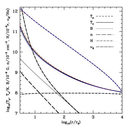
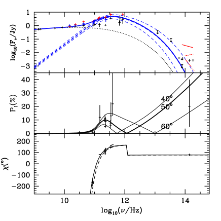
Figure 1: Left: Profiles of the electron (solid), proton (dashed) temperatures, magnetic field (dotted), gas density (long dashed), scale height (dot-dashed), and $\nu_{E}$ (dot-long-dashed) for the fiducial model with $\beta_{\nu}=0.7$, $\beta_{p}=0.4$, $C_{1}=0.38$, $\dot{M}=4.0\times 10^{17}$ g s^-1, $i=50^{\circ}$, and $T_{e}=T_{p}=GMm_{p}/5k_{\rm B}r$ at the outer boundary. The thin dashed and solid lines show the temperature profiles for $C_{1}=0.36$ and $0.40$, respectively. The other parameters don’t change, and profiles of other quantities change very little. Right: Model fit to the broadband spectrum and linear polarization. The top panel shows the fitting to the spectrum (Liu et al. 2004). The spectra of NIR flares are from recent observations [Gillessen et al. 2006 (dotted); Hornstein 2007 (solid)]. The dotted line corresponds to an unpolarized component with $F_{\nu}=(\nu/10^{9.5}{\rm Hz})^{0.3}\exp[-(\nu/10^{10.5}{\rm Hz})^{1/3}]$ Jy. The thick dashed line fits the millimeter to NIR spectrum with the fiducial model. The thick solid line is the sum of the two. The thin dashed lines are for the two profiles with $C_{1}=0.36$ (with a higher flux) and $0.40$. The middle panel compares the polarization fractions. The data are from Aitken et al. (2000), Macquart et al. (2006), and Marrone et al. (2007). The thick line is for the fiducial model. The thin lines have $i=60^{\circ}$ (with a higher millimeter and sub-millimeter polarization) and $40^{\circ}$. Bottom: the observed position angle of the linear polarization for the fiducial model. The rotation axis of the disk has a position angle of $168^{\circ}$. The solid and dashed lines assume an external Faraday rotation measure of -44 and -56 rad cm^-2, respectively (Macquart et al. 2006; Marrone et al. 2007). According to the model, the position angle of the polarization flips by $90^{\circ}$ in the sub-millimeter range at the frequency, where the polarization fraction approaches to 0.

For given $\beta_{\nu}$, $\beta_{p}$, $\dot{M}$, $C_{1}$, and $T_{e}$ and $T_{p}$ at an outer boundary, one can solve equations (3) and (4) numerically to obtain the disk structure. The thick lines in the left panel of Figure 1 give profiles of the fiducial model, where $\beta_{\nu}=0.7$, $\beta_{p}=0.4$, $\dot{M}=4.0\times 10^{17}$g s^-1, $C_{1}=0.38$, and $T_{e}=T_{p}=GMm_{p}/5k_{\rm B}r$ at the outer boundary $r=10^{4}r_{S}$. For such a low accretion rate, cooling is not very efficient and the temperature profiles are determined by the electron heating rate. The thin solid and dashed lines give the temperature profiles for $C_{1}=0.40$ and $0.36$, respectively. The other model parameters remain the same. Due to the increase of the electron heating rate, the electron temperature is higher for the latter, which has a slightly lower proton temperature for energy conservation. The profiles of other quantities do not change significantly. We note that the disk structure at small radii is very sensitive to the stress at the inner boundary $3r_{S}$. Here the stress is chosen such that there is no net angular momentum flux through the disk, which is appropriate for strongly magnetized disks.

3 Radiation Spectrum and Polarization

The formulae for calculating polarized synchrotron emission are given by Melia et al. (2001), who treat the flow as a slim disk. Since the millimeter and shorter wavelength emissions are mostly produced within 10 $r_{S}$, where electrons are relativistic, as indicated by the profiles of $\nu_{E}$ and $T_{e}$, the emission and absorption are dominated by the extraordinary emission component and the Faraday conversion dominates the Faraday rotation in the millimeter and sub-millimeter bands (Melrose 1997). Then the emission, absorption, and dispersion vectors defined by Landi Degl’Innocenti and Landolfi (2004) are in the same direction. With the slim disk approximation, the plasma is uniform along a light ray and the dispersion effects can be neglected. So the formulae given by Melia et al. (2001) remain valid. Considering the vertical structure of the disk and the inhomogeneities caused by turbulence may reduce the level of linear polarization and induce circular polarization as implied by equations 5.74a and 5.74b of Landi Degl’Innocenti and Landolfi (2004).

A recent study of the magneto-rotational-instability indicates that $\beta_{\nu}\simeq 0.7$ when the turbulence saturates (Pessah et al. 2006). In principle, $\beta_{p}$ can also be determined by realistic MHD simulations. Then the observed spectrum and polarization can give tight constraints on the disk inclination angle $i$ and $C_{1}$. The right panel of Figure 1 compares the model predicted spectrum and linear polarization with observations. The thick dashed line in the top panel gives the spectrum of the fiducial model with $i=50^{\circ}$, which fits the millimeter to NIR spectrum. The spectral index below $100$ GHz is $\sim 1.7$, which is determined by the structure of the disk. Emission from different radii peaks at different frequencies, above which the source becomes optically thin, and lower frequency emission is produced at relatively larger radii. The dotted line fit the low frequency spectrum with $F_{\nu}=(\nu/10^{9.5}{\rm Hz})^{0.3}\exp[-(\nu/10^{10.5}{\rm Hz})^{1/3}]$ Jy. As mentioned in the introduction, this component is likely associated with an outflow and its linear polarization is negligible (Bower et al. 2002). The thick solid line is the sum of the two, which fits the broadband spectrum.

Although most of the emission from the disk is produced in the optically thin regime, the linear polarization at lower frequencies is suppressed due to the dominance of the unpolarized component. The polarization is significant only in the millimeter and shorter wavelength range as shown in the middle panel, where the thick line corresponds to the fiducial model, and the two thin lines have $i=40^{\circ}$ and $60^{\circ}$. The polarization fraction in the sub-millimeter range increases dramatically with the increase of $i$. Our fitting to the observations gives an $i$ of $\sim 50^{\circ}\pm 10^{\circ}$. More accurate polarization observations above $300$ GHz may give a better measurement of this angle.

The thin dashed lines in the top panel give the spectra for the two profiles with $C_{1}=0.36$ and $0.40$. The emission spectrum, especially in the NIR band, is very sensitive to the electron heating rate. A good measurement of Sagittarius A*’s quiescent flux in the NIR band can lead to an accurate determination of $C_{1}$ (Ghez et al. 2005b; Clénet et al. 2004). The model predicts an NIR spectral index of $\sim-3.5$. Any evidence of a harder quiescent NIR spectrum would suggest a non-thermal emission component.

Observations show that the position angle of the intrinsic polarization is $\sim 170^{\circ}$ (Macquart et al. 2006; Marrone et al. 2007). Our model predicts that the emission is polarized along the axis of the disk below $\sim 1200$ GHz. The axis of the disk therefore has a position angle of $\sim 170^{\circ}$. Future VLBI imaging may be able to test this prediction (Shen et al. 2005; Bromley et al. 2001; Huang et al. 2007). For small values of $i$, the model predicts that the position angle of the polarization flips by $90^{\circ}$ in the sub-millimeter range due to the dominance of the high frequency emission by the blue shifted side. We note that in the NIR band, where the emission is also dominated by the blue-shifted side, the corresponding position angle of the polarization is $\sim 80^{\circ}$, which is consistent with recent observations (Eckart et al. 2006b; Meyer et al. 2006). The bottom panel shows the fitting to the position angle of the observed linear polarization. Here an external Faraday rotation has been introduced following Macquart et al. (2006) and Marrone et al. (2007). Such an external Faraday rotation may originate from the outflow as suggested by Beckert and Falcke (2002).

4 Discussion and Conclusions

We have shown that the disk model can account for the millimeter spectrum and polarization, the $\sim 90^{\circ}$ difference in the position angle of the polarized sub-millimeter and NIR emissions. Our best-fit model predicts a $\sim 8\%$ polarization at 150 GHz, a very soft quiescent state NIR spectrum, and a disk inclination angle of $50^{\circ}$ with the axis aligning at $\sim 170^{\circ}$ position angle. Future polarimetric spectroscopy and imaging will be able to test the model and/or better constrain the parameters.

Since $\beta_{p}$ is currently not well determined by simulations, the fitting to the observed data is not unique. For $\beta_{\nu}=0.7$, $\beta_{p}=0.1$, $C_{1}=1.08$, $\dot{M}=2\times 10^{17}$g s^-1, and $i=50^{\circ}$, we obtain essentially the same emission spectrum and polarization from the disk as the fiducial model. A better constraint of $\beta_{p}$ by simulations is therefore critical to pin down the rest of the model parameters with simultaneous spectrum and polarization observations. The best-fit orientation of the disk is not sensitive to $\beta_{p}$. However, since most of the emission is produced near the last stable orbit $3r_{S}$, the stress at this radius and the emission from the plunging region may affect the best-fit value of $i$. A full general relativistic MHD simulation will not only address these issues and remove the parameters $\beta_{\nu}$ and $\beta_{p}$, but also treat the vertical structure of the disk and the effects of winds or outflows properly, which may explain the observed external Faraday rotation and the centimeter emission component (Liu & Melia 2001; Yuan et al. 2002; Sharma et al. 2007b). However, to apply MHD simulations to Sagittarius A* directly, one needs an advanced treatment of the electron heating by turbulence, takes into account the general relativistic light binding effects, and does the transfer of polarized emission in a turbulent flow properly. The plasma dispersion effects may induce circular polarization and introduce comparable modification to the spectrum and linear polarization as the general relativistic effects (Melrose 1997; Broderick & Blandford 2004). These investigations may eventually lead to a measurement of the black hole spin.

Compared with the previous models of a small hot accretion torus (Melia et al. 2001; Bromley et al. 2001), we make several significantly improvements. A more realistic treatment of electron heating by turbulence replaces the assumption of one temperature flow in the original model. This also makes the results almost independent of the outer boundary radius and temperature(s). With the pseudo-Newtonian potential, the inner radius is not a free parameter anymore and fixed at the last stable orbit. The zero stress inner boundary condition is replaced by the zero angular momentum flux condition. Although other models may also explain the observations studied in this paper (e.g. Yuan et al. 2002), the model presented here has less parameters and assumptions on the dynamics of the accretion flow and/or outflow and therefore likely reveals the dominant physical processes responsible for the observed emission.

References

- Agol et al. (2000) Agol, E. 2000, ApJ, 538, L121
- Aitken et al. (2000) Aitken, D. K., et al. 2000, ApJ, 534, L173
- An et al. (2005) An, T., et al. 2005, ApJ, 634, L49
- Baganoff et al. (2001) Baganoff, F. K., et al. 2001, Nature, 413, 45
- Bittner et al. (2007) Bittner, J. M., Liu, S., Fryer, C. L., & Petrosian, V. 2007, ApJ, 661, 863
- Beckert & Falcke (2002) Beckert, T., & Falcke, H. 2002, A&A, 388, 1106
- Bower et al. (2002) Bower, G. C., Falcke, H., Sault, R. J., & Backer, D. C. 2002, ApJ, 571, 843
- Bower et al. (2005) Bower, G. C., Falcke, H., Wright, M. C. H., & Backer, D. C. 2005, ApJ, 618, L29
- Broderick & Blandford (2004) Broderick, A. E., & Blandford, R. 2004, MNRAS, 349, 994
- Bromley et al. (2001) Bromley, B., Melia, F., & Liu, S. 2001, ApJ, 555, L83
- Clenet et al. (2004) Clénet, Y., et al. 2004, A&A, 424, L21
- Eckart et al. (2006a) Eckart, A., et al. 2006a, A&A, 450, 535
- Eckart et al. (2006b) Eckart, A., Schödel, R., Meyer, L., Tripper, S., Ott, T., & Genzel, R. 2006b, A&A, 455, 1
- Falcke et al. (1998) Falcke, H., Goss, W. M., Matsuo, H., Teuben, P., Zhao, J.-H., & Zylka, R. 1998, ApJ, 499, 73
- Genzel, et al. (2003) Genzel, R. et al. 2003, Nature, 425, 934
- (16) Ghez, A. M., et al. 2005a, ApJ, 620, 744
- (17) – – –. 2005b, ApJ, 635, 1087
- Gillessen et al. (2006) Gillessen S., et al. 2006, ApJ, 640, 163L
- Hornstein et al. (2007) Hornstein, S. D., et al. 2007, ApJ, astro-ph/0706.1782
- Huang et al. (2007) Huang, L., Cai, M., Shen, Z. Q., & Yuan, F. 2007, MNRAS, in press, astro-ph/0703254
- Landi et al. (2004) Landi Degl’Innocenti, E., & Landolfi, M. 2004, Polarization in Spectral Lines, (Kluwer Academic Publishers), p176-p179
- Liu & Melia (2001) Liu, S., & Melia, F. 2001, ApJ, 561, L77
- Liu, Petrosian, & Melia (2004) Liu, S., Petrosian, V., & Melia, F. 2004, ApJ, 611, L101
- Liu et al. (2006) Liu, S., Petrosian, V., Melia, F., & Fryer, C. L. 2006, ApJ, 648, 1020
- Liu et al. (2007) Liu S. et al. 2007, ApJ, Submitted, astro-ph/0705.0525
- Macquart et al. (2006) Macquart, J. Bower, G. C., Wright, M. C. H., Backer, D. C. & Falcke, H. 2006, ApJ, 646, L111
- (27) Marrone, D. P., Moran, J. M., Zhao, J. H., & Rao, R. 2006a, ApJ, 640, 308
- (28) – – –. 2006b, Journal of Physics: Conference Series, 54, 354, astro-ph/0607432
- Marrone et al. (2007) – – –. 2007, ApJ, 654, L57
- Melia (1992) Melia, F. 1992, ApJ, 387, L25
- Melia et al. (2000) Melia, F., Liu, S., & Coker, R. 2000, ApJ, 545, L117
- Melia et al. (2001) – – –. 2001, ApJ, 553, 146
- Melrose (1997) Melrose, D. B., 1997, J. Plasma Physics, 58, 735
- Meyer et al. (2006) Meyer, L., Schödel, L., Eckart, A., Karas, V., Dovčiak, & Duschl, W. J. 2006, A&A, 458, 25
- Narayan et al. (1998) Narayan, R., et al. 1998, ApJ, 492, 554
- Pessah et al. (2006) Pessah, M. E., Chan, C. K., & Psaltis, D. 2006, PRL 97, 221103
- Quataert et al. (2000) Quataert, E., & Gruzinov, A. 2000, ApJ, 545, 842
- Rockefeller et al. (2004) Rockefeller, G., Fryer, C. L., Melia, F., & Warren, M. S. 2004, ApJ, 604, 662
- Schodel et al. (2002) Schödel, R., et al. 2002, Nature, 419, 694
- Sharma et al. (2007a) Sharma, P., Quataert, E., Hammett, G. W., & Stone, J. M. 2007, ApJ, Submitted, astro-ph/0703572
- Sharma et al. (2007b) Sharma, P., Quataert, E., & Stone, J. M. 2007, ApJ, Submitted, astro-ph/0706.3715
- Shen et al. (2005) Shen, Z.-Q., Lo, K. Y., Liang, M.-C., Ho, P. T. P., & Zhao, J.-H. 2005, Nature, 438, 62
- Spitzer (1990) Spitzer, L. 1990, Physics of Fully Ionized Gases, (Dover Publications, Inc. Mineola, New York), p135
- Yuan et al. (2002) Yuan, F., Markoff, S., & Falcke, H., 2002, A&A, 383, 854
- (45) Yusef-Zadeh, F., et al. 2006a, ApJ, 644, 198
- Yusef-Zadeh et al. (2006b) – – –. 2006b, ApJ, 650, 189
- Zhao et al. (2004) Zhao, J. H., Herrnstein, R. M., Bower, G. C., Goss, W. M., & Liu, S. M. 2004, ApJ, 603, L85