Homogenized spectral problems for exactly solvable operators: asymptotics of
polynomial eigenfunctions

Abstract.

Consider a homogenized spectral pencil of exactly solvable linear differential operators $T_{\lambda}=\sum_{i=0}^{k}Q_{i}(z)\lambda^{k-i}\frac{d^{i}}{dz^{i}}$, where each $Q_{i}(z)$ is a polynomial of degree at most $i$ and $\lambda$ is the spectral parameter. We show that under mild nondegeneracy assumptions for all sufficiently large positive integers $n$ there exist exactly $k$ distinct values $\lambda_{n,j}$, $1\leq j\leq k$, of the spectral parameter $\lambda$ such that the operator $T_{\lambda}$ has a polynomial eigenfunction $p_{n,j}(z)$ of degree $n$. These eigenfunctions split into $k$ different families according to the asymptotic behavior of their eigenvalues. We conjecture and prove sequential versions of three fundamental properties: the limits $\Psi_{j}(z)=\lim_{n\to\infty}\frac{p_{n,j}^{\prime}(z)}{\lambda_{n,j}p_{n,j}(z)}$ exist, are analytic and satisfy the algebraic equation $\sum_{i=0}^{k}Q_{i}(z)\Psi_{j}^{i}(z)=0$ almost everywhere in $\mathbb{CP}^{1}$. As a consequence we obtain a class of algebraic functions possessing a branch near $\infty\in\mathbb{CP}^{1}$ which is representable as the Cauchy transform of a compactly supported probability measure.

1. Introduction and main results

In this paper we study the properties of asymptotic root-counting measures for families of (nonstandard) polynomial eigenfunctions of exactly solvable linear differential operators. Using this information we describe a class of algebraic functions possessing a branch near $\infty\in\mathbb{CP}^{1}$ which is representable (up to a constant factor) as the Cauchy transform of a compactly supported probability measure.

Notation 1.

A linear ordinary differential operator $T:=\sum_{i=1}^{k}a_{i}(z)\frac{d^{i}}{dz^{i}}$ is called exactly solvable or ES for short if $T$ (nonstrictly) preserves the infinite flag $\mathcal{P}_{0}\subset\mathcal{P}_{1}\subset\mathcal{P}_{2}\subset\ldots$, where $\mathcal{P}_{i}$ denotes the linear space of polynomials in $z$ of degree at most $i$, see [27].

The well-known classification theorem of S. Bochner, see [9] and [21], states that each coefficient $a_{i}(z)$ of an exactly solvable $T$ is a polynomial of degree at most $i$.

$T$ is called strictly exactly solvable if the flag $\mathcal{P}_{0}\subset\mathcal{P}_{1}\subset\mathcal{P}_{2}\subset\ldots$ is strictly preserved. One can show that the coefficients $a_{i}(z):=\sum_{j=0}^{i}a_{i,j}z^{j}$ of a strictly exactly solvable $T$ satisfy the condition that the equation $\sum a_{i,i}t(t-1)\ldots(t-i+1)=0$ has no positive integer solutions, see Lemma 2.1 below.

Finally, let $ES_{k}$ denote the linear space of all $ES$-operators of order at most $k$.

Consider a spectral pencil of $ES_{k}$-operators $T_{\lambda}:=\sum_{i=0}^{k}a_{i}(z,\lambda)\frac{d^{i}}{dz^{i}}$, i.e., a parametrized curve $T:\mathbb{C}\to ES_{k}$. Each value of the parameter $\lambda$ for which the equation $T_{\lambda}p(z)=0$ has a polynomial solution is called a (generalized) eigenvalue and the corresponding polynomial solution is called a (generalized) eigenpolynomial.

The main problem that we address in this paper is as follows.

Problem 1.

Given a spectral pencil $T_{\lambda}$ describe the asymptotics of its eigenvalues and the asymptotics of the root distribution of the corresponding eigenpolynomials.

Motivated by the necessities of the asymptotic theory of linear ordinary differential equations, see e.g. [15, Ch. 5], we concentrate below on the fundamental special case of homogenized spectral pencils, i.e., rational normal curves in $ES_{k}$ of the form

$$T_{\lambda}=\sum_{i=0}^{k}Q_{i}(z)\lambda^{k-i}\frac{d^{i}}{dz^{i}},$$ (1.1)

where each $Q_{i}(z)$ is a polynomial of degree at most $i$. Consider the algebraic curve $\Gamma$ given by the equation

$$\sum_{i=0}^{k}Q_{i}(z)w^{i}=0,$$ (1.2)

where the polynomials $Q_{i}(z)=\sum_{j=0}^{i}a_{i,j}z^{j}$ are the same as in (1.1). Given a curve $\Gamma$ as in (1.2) and the pencil $T_{\lambda}$ as in (1.1) with the same coefficients $Q_{i}(z)$, $0\leq i\leq k$, we call $\Gamma$ the plane curve associated with $T_{\lambda}$ and we say that $T_{\lambda}$ is the spectral pencil associated with $\Gamma$.

The curve $\Gamma$ and its associated pencil $T_{\lambda}$ are called of general type if the following two nondegeneracy requirements are satisfied:

• $\deg Q_{k}(z)=k$ (i.e., $a_{k,k}\neq 0$),

• no two roots of the (characteristic) equation

  $$a_{k,k}+a_{k-1,k-1}t+\ldots+a_{0,0}t^{k}=0$$ (1.3)

  lie on a line through the origin (in particular, $0$ is not a root of (1.3)).

The first statement of the paper is as follows.

Proposition 1.

If the characteristic equation (1.3) has $k$ distinct solutions $\alpha_{1},\alpha_{2},$ $\ldots,\alpha_{k}$ and satisfies the preceding nondegeneracy assumptions (in particular, these imply that $a_{0,0}\neq 0$ and $a_{k,k}\neq 0$) then

• for all sufficiently large $n$ there exist exactly $k$ distinct eigenvalues $\lambda_{n,j}$, $j=1,\ldots,k$, such that the associated spectral pencil $T_{\lambda}$ has a polynomial eigenfunction $p_{n,j}(z)$ of degree exactly $n$,

• the eigenvalues $\lambda_{n,j}$ split into $k$ distinct families labeled by the roots of (1.3) such that the eigenvalues in the $j$-th family satisfy

  $$\lim_{n\to\infty}\frac{\lambda_{n,j}}{n}=\alpha_{j},\quad j=1,\ldots,k.$$

Theorem 1.

In the notation of Proposition 1 for any pencil $T_{\lambda}$ of general type and every $j=1,\ldots,k$ there exists a subsequence $\{n_{i,j}\}$, $i=1,2,\ldots,$ such that the limits

$$\Psi_{j}(z):=\lim_{i\to\infty}\frac{p_{n_{i,j}}^{\prime}(z)}{\lambda_{n_{i,j}}p_{n_{i,j}}(z)},\quad j=1,\ldots,k,$$

exist almost everywhere in $\mathbb{C}$ and are analytic functions in some neighborhood of $\infty$. Each $\Psi_{j}(z)$ satisfies equation (1.2), i.e., $\sum_{i=0}^{k}Q_{i}(z)\Psi_{j}^{i}(z)=0$ almost everywhere in $\mathbb{C}$, and the functions $\Psi_{1}(z),\ldots,\Psi_{k}(z)$ are independent sections of $\Gamma$ considered as a branched covering over $\mathbb{CP}^{1}$ in a sufficiently small neighborhood of $\infty$.

As we explain in §5, a key ingredient in the proof of Theorem 1 is the following localization result for the roots of the above eigenpolynomials.

Theorem 2.

For any general type pencil $T_{\lambda}$ all the roots of all its polynomial eigenfunctions $p_{n,j}(z)$ lie in a certain disk in $\mathbb{C}$ centered at the origin.

The sketch of the proof of this fundamental result is as follows. We convert the differential equation satisfied by the eigenpolynomials into a non-linear Riccati type equation for the logarithmic derivatives of the eigenpolynomials. This equation is then solved recursively and the formal solution is shown to be analytic in a neighborhood of $\infty$. This shows that the zeros of the eigenpolynomials (coinciding with the poles of the logarithmic derivatives) must lie in some compact subset of $\mathbb{C}$.

Moreover, we conjecture that for each $j$ the above convergence result holds in fact for the whole corresponding sequence of eigenpolynomials.

Conjecture 1.

In the notation of Theorem 1, for every $j=1,\ldots,k$ the limit

$$\Psi_{j}(z)=\lim_{n\to\infty}\frac{p_{n,j}^{\prime}(z)}{\lambda_{n,j}p_{n,j}(z)}$$

exists and has all the properties stated in Theorem 1 almost everywhere in $\mathbb{CP}^{1}$.

We emphasize the fact that the proof of Theorem 1 actually shows that Conjecture 1 is valid (at least) in a neighborhood of infinity.

In order to formulate our further results and reinterpret Theorems 1–2 and Conjecture 1 we need some notation and several basic notions of potential theory.

Notation 2.

The function $L_{n,j}(z)=\frac{p_{n,j}^{\prime}(z)}{\lambda_{n,j}p_{n,j}(z)}$ is called the normalized logarithmic derivative of the polynomial $p_{n,j}(z)$. The limit $\Psi_{j}(z)=\lim_{n\to\infty}L_{n,j}(z)$ (if it exists) will be referred to as the asymptotic (normalized) logarithmic derivate of the family $\{p_{n,j}(z)\}$.

The root-counting measure $\mu_{P}$ of a given polynomial $P(z)$ of degree $m$ is the finite probability measure obtained by placing the mass $\frac{1}{m}$ at every root of $P(z)$. (If some root is multiple we place at this point the mass equal to its multiplicity divided by $m$.) Given a sequence $\{P_{m}(z)\}$ of polynomials we call the limit $\mu=\lim_{m\to\infty}\mu_{P_{m}}$ (if it exists in the sense of the weak convergence of functionals) the asymptotic root-counting measure of the sequence $\{P_{m}(z)\}$.

If $\mu$ exists and is compactly supported it is also a probability measure and its support $\mathrm{s}upp~{}\mu$ is the limit (in the set-theoretic sense) of the sequence $\{\mathcal{Z}_{P_{m}}\}$ of the zero loci to $\{P_{m}(z)\}$.

The Cauchy transform of a complex-valued compactly supported finite measure $\rho$ is given by

$$C_{\rho}(z)=\int_{\mathbb{C}}\frac{d\rho(\xi)}{z-\xi}.$$

Note that $C_{\rho}(z)$ is defined at each point $z$ for which the Newtonian potential

$$U_{|\rho|}(z)=\int_{\mathbb{C}}\frac{d|\rho|(\zeta)}{|\zeta-z|}$$

is finite. It is easy to see that $C_{\rho}(z)$ exists a.e. and that the original measure $\rho$ can be restored from its Cauchy transform by the formula

$$\rho=\frac{1}{\pi}\frac{\partial C_{\rho}(z)}{\partial\bar{z}},$$

where $\frac{1}{\pi}\frac{\partial C_{\rho}(z)}{\partial\bar{z}}$ is considered as a distribution, see e.g. [16, Ch. 2].

Note also that the Cauchy transform $C_{\mu_{P}}(z)$ of the root-counting measure $\mu_{P}$ of a given degree $m$ polynomial $P(z)$ coincides with $\frac{P^{\prime}}{mP}$.

A reinterpretation of Theorem 1 in the above terms is as follows.

Proposition 2.

In the notation of Theorem 1, for each $j=1,\ldots,k$ there exists a subsequence $\{n_{i,j}\}$, $i=1,2,\ldots$, such that the asymptotic root-counting measure $\mu_{j}$ of the family $\{p_{n_{i,j}}(z)\}_{i}$ exists and has compact support with vanishing Lebesgue area. The Cauchy transform of $\mu_{j}$ coincides with $\alpha_{j}\Psi_{j}$ almost everywhere in $\mathbb{C}$.

As an illustration we present below some numerical results showing a rather complicated behavior of the zero loci $\mathcal{Z}_{p_{n,j}}$ for $j=1,\ldots,k$. Recall that $\mathrm{s}upp~{}\mu_{j}=\lim_{n\to\infty}\mathcal{Z}_{p_{n,j}}$ and note that there are slight differences between the scalings used in the four pictures shown in Fig. 1.

         

         

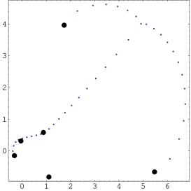
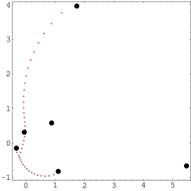
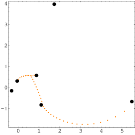
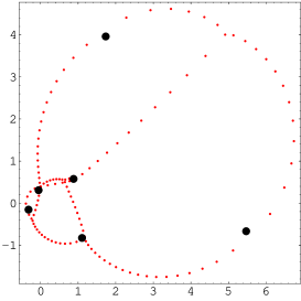
Figure 1. Three root-counting measures for a third order homogenized spectral pencil.

Explanations to Fig. 1. The two pictures in the upper row and the left picture in the bottom row show the roots of three eigenpolynomials of degree $55$ for the (ad hoc chosen) homogenized spectral pencil

$$T_{\lambda}=\left(z^{3}-(5+2I)z^{2}+(4+2I)z\right)\frac{d^{3}}{dz^{3}}+\lambda(z^{2}+Iz+2)\frac{d^{2}}{dz^{2}}+\lambda^{2}\frac{1}{5}(z-2+I)\frac{d}{dz}+\lambda^{3}$$

consisting of $ES_{3}$-operators. The remaining picture shows the union of the roots of all three polynomials. The six fat points on all pictures are the branching points of the associated algebraic curve $\Gamma$ given by

$$\left(z^{3}-(5+2I)z^{2}+(4+2I)z\right)w^{3}+(z^{2}+Iz+2)w^{2}+\frac{1}{5}(z-2+I)w+1=0$$

and considered as the branched covering over the $z$-plane. Numerical comparisons of the eigenfunctions of different degrees show that the above three root distributions already give a very good approximation of the three corresponding limiting probability measures $\mu_{1},\mu_{2},\mu_{3}$ whose Cauchy transforms generate (after appropriate scalings, see Theorem 1) the three branches of $\Gamma$ near $\infty$. Note that all three supports end only at the six branching points of $\Gamma$.

As far as the measures $\mu_{j}$ are concerned, in this paper we establish just some of their most important properties. To prove these we use two facts about $C_{\mu_{j}}(z)$. First, that $\alpha_{j}^{-1}C_{\mu_{j}}(z)$ satisfies the algebraic equation (1.2) and hence can be locally written as a finite sum $\sum_{i=1}^{r}\chi_{i}\alpha_{i}^{-1}\Psi_{i}$, where the $\chi_{i}$’s are characteristic functions of certain sets. Second, that

$$\frac{\partial C_{\mu_{j}}(z)}{\partial\bar{z}}\geq 0$$

in the sense of distributions. Using these facts we can develop a natural algebraic geometric setting and build on complex analytic techniques based on the main results of [10] in order to prove the next two theorems.

Theorem 3.

For each pencil $T_{\lambda}$ of general type there exists a real-analytic subset $\Gamma_{2}$ of ${\mathbb{C}}$ such that any limiting measure $\mu_{j}$ has properties (A)–(C) below in any sufficiently small neighborhood $\Omega(z_{0})$ of any point $z_{0}\in{\mathbb{C}}\setminus\Gamma_{2}$. In what follows $\Gamma$ denotes the curve associated with the pencil $T_{\lambda}$, $\alpha_{j}\in\bf C$ is as in Proposition 1, and for any branch $\gamma_{i}$ of $\Gamma$ we let $A_{i}:=\alpha_{j}\gamma_{i}$ (clearly, $A_{i}$ depends on $j$).

• The support $S$ of the measure $\mu_{j}$ restricted to $\Omega(z_{0})$ is a finite union of smooth curves $S_{r},\ r\in J$.

• For each $S_{r}$ and any $\tilde{z}\in S_{r}$ lying in $\Omega(z_{0})$ one can always choose two branches $\gamma_{1}(z)$ and $\gamma_{2}(z)$ of $\Gamma$ such that the tangent line $l(\tilde{z})$ to $S_{r}$ is orthogonal to $\overline{A_{1}(\tilde{z})}-\overline{A_{2}(\tilde{z})}$.

• The density of the measure $\mu_{j}$ at $\tilde{z}$ equals $\frac{|{A_{1}(\tilde{z}})-A_{2}({\tilde{z}})|ds}{2\pi}$, where $ds$ is the length element along the curve $S_{r}$.

In fact for most pencils we can do better:

Theorem 4.

For a typical general type pencil $T_{\lambda}$ the set $\Gamma_{2}$ in the preceding theorem is finite.

Remark 1.

In the case of the usual spectral problem strong results in this direction were obtained in [4].

We note that Theorem 1 also leads to a partial progress on the following intriguing question in potential theory. Let $Alg(i,j)$ denote the linear space of all polynomials in the variables $(y,z)$ of bidegrees at most $(i,j)$, i.e., each $P(y,z)\in Alg(i,j)$ has the form $\sum_{l=0}^{i}P_{l}(z)y^{l}$, where $\deg P_{l}(z)\leq j,\;l=1,\ldots,i$. Abusing the notation we identify each $P(y,z)\not\equiv 0$ with the algebraic function in the variable $z$ defined by the equation $P(y,z)=0$.

Problem 2.

Describe the subset $PAlg(i,j)\subset Alg(i,j)$ consisting of all algebraic functions which have a branch near $\infty$ coinciding with the Cauchy transform of some probability measure compactly supported in $\mathbb{C}$.

We refer to such algebraic functions as positive Cauchy transforms. The only case when a complete answer to the above problem seems to be obvious is for bidegrees $(1,j)$, i.e., the case of rational functions. Namely, a rational function $r(z)=\frac{p(z)}{q(z)}$ is a positive Cauchy transform if and only if $r(z)$ is of the form

$$\sum_{l=1}^{j}\frac{c_{l}}{z-z_{l}}\text{ with }c_{l}>0,1\leq l\leq j,\,z_{k}\neq z_{l}\text{ for }k\neq l,\,\sum_{l=1}^{j}c_{l}=1.$$

Let us finally give yet another interpretation of Theorem 1 and Proposition 2.

Corollary 1.

Each branch near infinity of an algebraic function satisfying (1.2) is a positive Cauchy transform multiplied by an appropriate constant.

The structure of the paper is as follows. In §2 we study the asymptotics of the eigenvalues to (1.1) and some simple properties of the corresponding eigenfunctions as well as the defining algebraic curve (1.2). In §3 we solve the spectral problem defined by the operator (1.1) in formal power series near $\infty$ using the variable $y:=z^{-1}$. In §4 we show that the power series solution obtained in §3 converges in some neighborhood of $\infty$. Based on these results we prove Theorem 2 as well as Theorem 1 and its corollaries in §5. In §6 we prove Theorem 3 and complete the proof of Theorem 4. Finally, in §7 we propose a number of open problems and conjectures on the asymptotic behavior of polynomials functions for linear ordinary differential operators and place these in a wider context that encompasses both old and new literature on this and related topics.

Acknowledgements. We wish to thank Hans Rullgård for stimulating discussions on these subjects. It is difficult to underestimate the role of the excellent paper [4] in the current project. We would also like to thank the anonymous referee for his valuable comments.

2. Basic facts on asymptotics of eigenvalues and polynomial eigenfunctions

In this section we prove Proposition 1, that is, we describe the polynomial solutions of an $ES$ spectral pencil and we also prove the easy part of Theorem 1 saying that if the limit functions $\Psi_{j}(z)$, $1\leq j\leq k$, exist locally and have derivatives of sufficiently high order then they must satisfy equation (1.2).

Denote by $\mathcal{D}_{n}\subset ES_{k}$ the subset of all $ES$-operators $T$ of order at most $k$ such that the equation $Ty=0$ has a polynomial solution of degree exactly $n$.

Lemma 1.

In the notation of Theorem 1 the closure $\overline{\mathcal{D}_{n}}$ of the discriminant $\mathcal{D}_{n}$ is a hyperplane in $ES_{k}$ given by the equation

$$\sum_{i=0}^{k}n(n-1)\ldots(n-i+1)a_{i,i}=0.$$ (2.1)

Proof.

Since any $ES$-operator $T$ (nonstrictly) preserves the infinite flag $\mathcal{P}_{0}\subset\mathcal{P}_{1}\subset\ldots\subset\ldots$ of linear spaces of polynomials of at most given degree it follows that $T$ has an eigenpolynomial of degree exactly $n$ if and only if

• $T$ restricted to $\mathcal{P}_{n}$ is degenerate,

• the kernel of $T$ restricted to $\mathcal{P}_{n}$ intersects $\mathcal{P}_{n}\setminus\mathcal{P}_{n-1}$.

The closure $\overline{\mathcal{D}_{n}}$ consists of all $T$ having an eigenpolynomial of degree at most $n$. Now $T$ is upper triangular in the standard monomial basis and the $j$-th diagonal entry of $T$ equals $\sum_{i=0}^{k}j(j-1)\ldots(j-i+1)a_{i,i}$. Therefore $\overline{\mathcal{D}_{n}}$ is given by equation (2.1). ∎

Remark 2.

If $T\in\overline{\mathcal{D}_{n}}$ but $T\notin\overline{\mathcal{D}_{l}}$ for $0\leq l<n$ then $T$ has a polynomial solution of degree exactly $n$. Otherwise $T$ has at least a polynomial solution of degree equal to $\min\{l\in\{0,\ldots,n-1\}:T\in\overline{\mathcal{D}_{l}}\}$ (and probably some other polynomial solutions as well).

We now turn to Proposition 1.

Proof.

By Lemma 2.1 the homogenized spectral pencil $T_{\lambda}$ has a polynomial solution of degree at most $n$ if

$$\sum_{i=0}^{k}n(n-1)\ldots(n-i+1)a_{i,i}\lambda^{k-i}=0.$$ (2.2)

This equation is of degree exactly $k$ in $\lambda$ since $a_{0,0}\neq 0$. Considering $n$ for the moment as a complex variable, the equation defines an algebraic curve in $\mathbb{C}^{2}$ with $k$ branches over $\mathbb{C}$. The behavior of the branches at infinity may be found by substituting $\widetilde{\lambda}=\lambda/n$ and dividing the left-hand side of (2.2) by $n^{k}$, which gives

$$\sum_{i=0}^{k}1\cdot\frac{(n-1)}{n}\cdot\frac{(n-2)}{n}\cdot\ldots\cdot\frac{(n-i+1)}{n}\cdot a_{i,i}\cdot\widetilde{\lambda}^{k-i}=0.$$ (2.3)

If $n\to\infty$ the latter family of equations tends coefficientwise to equation (1.3). Since the latter has exactly $k$ different solutions, this is true for (2.3) as well if $n\in N$ for some simply connected neighborhood $N\subset\mathbb{CP}^{1}$ of infinity. Hence in $N$ there are $k$ different branches $\widetilde{\lambda}_{n,1},\ldots,\widetilde{\lambda}_{n,k}$ of the algebraic function $\widetilde{\lambda}$ defined as a function of the complex variable $n$ by equation (2.3), and corresponding branches $\lambda_{n,1},\ldots,\lambda_{n,k}$ of the algebraic function $\lambda$. Then clearly one has

$$\lim_{n\to\infty}\lambda_{n,j}/n=\lim_{n\to\infty}\widetilde{\lambda}_{n,j}=\alpha_{j},\quad j=1,\ldots,k.$$

This completes the proof of part (ii). To prove further that for each branch $\lambda_{n,j}$, $j=1,\ldots,k$, the associated spectral pencil $T_{\lambda}$ has a polynomial eigenfunction $p_{n,j}(z)$ of degree exactly $n$, we need to show that for a $\lambda$ and $n$ that solve equation (2.2) there is no $m\neq n$ such that $\lambda$ solves equation (2.2) for that $m$. This follows if we first prove that there are no solutions $n\neq m$ to $\lambda_{n,j}=\lambda_{m,j}$, $j=1,\ldots,k$, and secondly that if $j_{1}\neq j_{2}$ then there are no solutions to $\lambda_{n,j_{1}}=\lambda_{m,j_{2}}$ (both statements in a possibly shrunk neighborhood of infinity). The first statement is an immediate consequence of the assumptions since they imply that $\alpha_{j}\neq 0$, $j=1,\ldots,k$, and thus for each $j$ the function $n\mapsto\lambda_{n,j}$ is one-to-one in a neighborhood of infinity. For the second statement argue by contradiction as follows. If the statement is false there are unbounded sequences of positive integers $n_{i},m_{i}$, $i=1,2,\ldots$ such that $\lambda_{n_{i},j_{1}}=\lambda_{m_{i},j_{2}}$ for all $i$. We may assume (by choosing a subsequence and possibly interchanging $j_{1}$ and $j_{2}$) that $\lim_{i\to\infty}m_{i}/n_{i}=r\in\mathbb{R}$. Hence

$$\alpha_{j_{1}}=\lim_{i\to\infty}\lambda_{n_{i},j_{1}}/n_{i}=\lim_{i\to\infty}(\lambda_{m_{i},j_{2}}/m_{i})(m_{i}/n_{i})=r\alpha_{j_{2}}$$

and so the arguments of $\alpha_{j_{1}}$ and $\alpha_{j_{2}}$ are equal, which contradicts the nondegeneracy assumptions in the proposition. This completes the proof. ∎

Remark 3.

It is possible and straightforward to calculate the asymptotics for the eigenvalues even in the case when (1.3) has multiple or vanishing roots.

Let us now prove the easy part of Theorem 1.

Proposition 3.

Let $\{p_{n,j}(z)\}$ be a family of polynomial eigenfunctions of a homogenized spectral pencil $T_{\lambda}$ with corresponding family of eigenvalues $\{\lambda_{n,j}\}$, i.e., $p_{n,j}(z)$ satisfies the equation $T_{\lambda_{n,j}}p_{n,j}(z)=0$. Assume that the following holds:

• $\lim_{n\to\infty}\lambda_{n,j}=\infty$,

• there exists an open set $\Omega\subseteq\mathbb{CP}^{1}$ where the normalized logarithmic derivatives $L_{n,j}(z)=\frac{p_{n,j}^{\prime}(z)}{\lambda_{n,j}p_{n,j}(z)}$ are defined for all sufficiently large $n$ and the sequence $\{L_{n,j}(z)\}$ converges in $\Omega$ to a function

  $$\Psi_{j}(z):=\lim_{n\to\infty}L_{n,j}(z),$$

• the $k-1$ first derivatives of the sequence $\{L_{n,j}(z)\}$ are uniformly bounded in $\Omega$.

Then if $\Psi_{j}(z)$ does not vanish identically it satisfies the equation

$$\sum_{i=0}^{k}Q_{i}(z)\Psi^{i}_{j}(z)=0.$$ (2.4)

Proof.

In order to simplify the notation in this proof let us fix the value of the index $j\in\{1,\ldots,k\}$ and simply drop it.

Note that each $L_{n}(z)=\frac{p_{n}^{\prime}(z)}{\lambda_{n}p_{n}(z)}$ is well defined and analytic in any disk $\mathbf{D}$ free from the zeros of $p_{n}(z)$. Choosing such a disk $\mathbf{D}$ and an appropriate branch of the logarithm such that $\log p_{n}(z)$ is defined in $\mathbf{D}$ let us consider a primitive function $M(z)=\lambda^{-1}_{n}\log p_{n}(z)$ which is also well defined and analytic in $\mathbf{D}$.

Straightforward calculations give: $e^{\lambda_{n}M(z)}=p_{n}(z),\;$ $p^{\prime}_{n}(z)=p_{n}(z)\lambda_{n}L_{n}(z)$, and $p^{\prime\prime}_{n}(z)=p_{n}(z)(\lambda^{2}_{n}L^{2}_{n}(z)+\lambda_{n}L_{n}^{\prime}(z))$. More generally,

$$\frac{d^{i}}{dz^{i}}(p_{n}(z))p_{n}(z)\left(\lambda^{i}_{n}L^{i}_{n}(z)+\lambda^{i-1}_{n}F_{i}(L_{n}(z),L^{\prime}_{n}(z),\ldots,L^{(i-1)}_{n}(z))\right),$$

where the second term

$$\lambda_{n}^{i-1}F_{i}(L_{n},L_{n}^{\prime},\ldots,L_{n}^{(i-1)})$$ (2.5)

is a polynomial of degree $i-1$ in $\lambda_{n}$. The equation $T_{\lambda_{n}}p_{n}(z)=0$ gives us

$$p_{n}(z)\left(\sum_{i=0}^{k}Q_{i}(z)\lambda_{n}^{k-i}\left(\lambda_{n}^{i}L_{n}^{i}(z)+\lambda_{n}^{i-1}F_{i}(L_{n}(z),L^{\prime}_{n}(z),\ldots,L^{(i-1)}_{n}(z))\right)\right)=0$$

or equivalently,

$$\lambda_{n}^{k}\sum_{i=0}^{k}Q_{i}(z)\left(L^{i}_{n}(z)+\lambda_{n}^{-1}F_{i}(L_{n}(z),L^{\prime}_{n}(z),\ldots,L^{(i-1)}_{n}(z))\right)=0.$$ (2.6)

Letting $n\to\infty$ and using the boundedness assumption for the first $k-1$ derivatives we get the required equation (2.4). ∎

We end this section by establishing an important property of the curve $\Gamma$ given by (1.2). Note that unless $Q_{k}(x)\equiv 0$ the curve $\Gamma$ is a $k$-sheeted branched covering of the $z$-plane. We want to describe the behavior of $\Gamma$ at infinity. Using a change of coordinate $y:=z^{-1}$ we can rewrite equation (1.2) as

$$\sum_{i=0}^{k}Q_{i}(z)w^{i}=\sum_{i=0}^{k}z^{-i}Q_{i}(z)(wz)^{i}=\sum_{i=0}^{k}P_{i}(y)\xi^{i}=0,$$

where

$$P_{i}(y)=z^{-i}Q_{i}(z)=\sum_{j=0}^{i}a_{ij}y^{i-j}$$

and $\xi:=wz=w/y$. Note also that at the point $y=0$ one gets the reciprocal characteristic equation

$$a_{k,k}\xi^{k}+a_{k-1,k-1}\xi^{k-1}+\ldots+a_{0,0}=0.$$ (2.7)

Remark 4.

The roots $\xi_{1},\ldots,\xi_{k}$ of (2.7) are the inverses of the roots $\alpha_{1},\ldots,\alpha_{k}$, respectively, of (1.3).

Using the above argument we get the following simple statement.

Lemma 2.

If the roots $\xi_{1},\ldots,\xi_{k}$ of equation (2.7) are pairwise distinct then there are $k$ branches $\gamma_{i}(z)$, $i=1,\ldots,k$, of the curve $\Gamma$ that are well defined in some common neighborhood of $z=\infty$. The $i$-th branch $\gamma_{i}(z)$ satisfies the normalization condition $\lim_{z\to\infty}z\gamma_{i}(z)=\xi_{i}.$

3. Solving equation (2.6) formally

This and the following two sections are completely devoted to the proof of Theorems 1 and 2. The sketch of the proof of Theorem 1 is as follows. In Proposition 3 of §2 we have transformed the linear differential equation for the eigenpolynomials into a non-linear Riccati type equation for the logarithmic derivative. In this section we first analyze closely the terms of this new equation. We then describe the recursion scheme for solving this equation formally in a neighborhood of infinity and see how the solutions behave when $\lambda\to\infty$. Finally, in the next section we show that there is a neighborhood of $z=\infty$ where the formal solutions are analytic and we complete the proofs of Theorems 1 and 2 in §5.

Throughout this section we use the variable $y:=1/z$ near $z=\infty$.

The differential algebra $A_{z,L}$. As the first step we describe the terms occurring in equation (2.6) more precisely. It is convenient to do this in a universal setting using the following infinitely generated free commutative $\mathbb{C}$-algebra (or rather the free differential algebra, cf. [20])

$$A_{z,L}:={\mathbb{C}}[\lambda,\lambda^{-1},z,z^{-1},L^{(0)},L^{(1)},L^{(2)},\ldots].$$

This algebra should be thought of as (a universal object) containing the terms in equation (2.6). Concrete instances can be obtained by specialization. In particular, the $L^{(i)}$’s correspond to the normalized logarithmic derivatives in (2.6).

Note that the monomials $\lambda^{i}z^{j}L^{I}$ form a basis of $A_{z,L}$ considered as a vector space, where for any multi-index $I=(i_{1},\ldots,i_{r})$ the symbol $L^{I}$ denotes the product

$$L^{I}=\prod_{s=1}^{r}L^{(i_{s})}.$$

It suffices to use multi-indices $I$ that are finite non-decreasing sequences of non-negative integers. Denote the set of all such multi-indices by $FS$. (By definition, $L^{(0)}:=L$.) Such index sequences may alternatively be thought of as finite multisets. In particular, we include the empty sequence $\emptyset$ in $FS$ and interpret $L^{\emptyset}:=1$. For a given multi-index $I$ define its modulus by $|I|=\sum_{s=1}^{r}i_{s}$ and its length by $lng(I)=r$. (By definition, $|\emptyset|:=0$ and $lng(\emptyset):=0$). For a given $I\in FS$ denote by $I_{+}$ the sequence obtained from $I$ by discarding all its $0$ elements.

$A_{z,L}$ is equipped with a natural derivation $D_{z}$ which is a prototype of $\frac{d}{dz}$. Namely, $D_{z}$ is uniquely defined by the relations: $D_{z}*\lambda=0$, $D_{z}*z=1$ and $D_{z}*L^{(i)}=L^{(i+1)}$. (We use the symbol “$*$” to denote the action of a differential operator as opposed to the product of differential operators. Note that the ring of differential operators generated by $A_{z,L}$ and $D_{z}$ acts on $A_{z,L}$.)

The normalized logarithmic derivative in the universal setting. We can next use $A_{z,L}$ to describe the relation between the derivatives of an eigenpolynomial and its normalized logarithmic derivative. This is done by defining a differential $A_{z,L}$-module. Consider the free rank one $A_{z,L}$-module $A_{z,L}e^{M}$, where $e^{M}$ is the generator. Define $D_{z}*e^{M}:=\lambda Le^{M}$ and extend the action of $D_{z}$ to the whole $A_{z,L}e^{M}$ using the Leibnitz rule. Note that this action intuitively just says that $L$ is the normalized logarithmic derivative $D_{z}*e^{M}/\lambda e^{M}$ of the generator $e^{M}$. The following lemma can be easily proved by induction.

Lemma 3.

In the above notation one has $(D_{z})^{i}*e^{M}=R_{i}e^{M},$ where $R_{0}=1$, $R_{1}=\lambda L$ and $R_{i+1}=(\lambda L+D_{z})*R_{i}$ for $i\geq 1$. In other words,

$$R_{i}=(\lambda L+D_{z})^{i}*1=(\lambda L+D_{z})^{i-1}*\lambda L,\quad i\geq 1.$$

The $R_{i}$ considered as polynomials $R_{i}(\lambda,L^{(0)},\ldots)$ have (by universality) the following property.

Lemma 4.

Let $g={\lambda}^{-1}{D\log f}$, where $f$ is a non-vanishing analytic function in an open subset $\Omega\subset{\mathbb{C}}$ and $\lambda\in{\mathbb{C}}\setminus\{0\}$ (so $g$ is the logarithmic derivative of $f$ normalized with respect to $\lambda$). Then in the above notation one has

$$f^{(i)}=R_{i}(\lambda,g,g^{(1)},\ldots.)f,\quad i\geq 1.$$

The differential algebra $A_{z,L}$ at $\infty$. Next we rewrite (2.6) using the variable $y=z^{-1}$. Note that if $p(z)$ is a non-constant polynomial then for any $\kappa\neq 0$ the logarithmic derivative $L(z)=p^{\prime}(z)/\kappa p(z)$, rewritten using the variable $y=\frac{1}{z}$, has a simple zero at $y=0$. Hence we should look for solutions of equation (2.6) in the form $L(z)=yN(y)$.

First we describe $A_{z,L}$ near $z=\infty$. For this we define an analogous free commutative algebra

$$B_{y,N}:={\mathbb{C}}[\lambda,\lambda^{-1},y,y^{-1},N^{(0)},N^{(1)},\ldots].$$

As above, it has a natural derivation $D_{y}$ which is a prototype of $\frac{d}{dy}$ satisfying the relations: $\,D_{y}*\lambda=0$, $D_{y}*y=1$ and $D_{y}*N^{(i)}=N^{(i+1)}$. Note that $\frac{d}{dz}=-y^{2}\frac{d}{dy}$ and recall that $L:=L^{(0)}$ and $N:=N^{(0)}$. Define an injection $\Theta:A_{z,L}\to B_{y,N}$ of algebras determined by

$$\Theta(\lambda)=\lambda,\,\Theta(z)=y^{-1},\,\Theta(L)=yN,\,\Theta(L^{(i)})=(-y^{2}D_{y})^{i}*yN.$$

The following lemma describes the connection between $A_{z,L}$ and $B_{y,N}$.

Lemma 5.

The injection $\Theta$ has the property that for any $a\in A_{z,L}$ one has

$$\Theta(D_{z}^{i}*a)=(-y^{2}D_{y})^{i}*\Theta(a).$$

Proof.

By definition the above formula is valid in the case $i=1$ for all the generators of $A_{z,L}$. Since $D_{z}$ and $-y^{2}D_{y}$ are derivations the formula then works for all elements in this algebra and $i=1$. Simple induction shows that the above formula is valid even for all $i>1$. ∎

Main lemma on $R_{i}$. The preceding lemmas imply the following relation:

$$\lambda^{-i}y^{-i}\Theta(R_{i})=y^{-i}(yN-y^{2}\lambda^{-1}D_{y})^{i}*1=y^{-i}(yN-y^{2}\lambda^{-1}D_{y})^{i-1}y*N.$$ (3.1)

We need to know which monomial terms of the form $\lambda^{\alpha_{1}}y^{\alpha_{2}}N^{I}$ occur in this equation. These monomials are contained in the subalgebra $B_{0}\subset B_{y,N}$ defined as

$$B_{0}:={\mathbb{C}}[\lambda^{-1},y,N,\lambda^{-1}yN^{(1)},\ldots,(\lambda^{-1}y)^{j}N^{(j)},\ldots],$$

see Lemma 6 below. Define a (necessarily two-sided, by commutativity) ideal $J\subset B_{0}$ as follows:

$$J:=<\lambda^{-1},(\lambda^{-1}y)^{2}N^{(1)}N^{(1)},\ldots,(\lambda^{-1}y)^{j_{1}+j_{2}}N^{(j_{1})}N^{(j_{2})}\ldots>,$$

where $j_{1}\geq 1,\;j_{2}\geq 1$. (As we will see the ideal $J$ contains all the terms that do not influence the asymptotic behavior of the equation (2.6).)

One can easily show that the set of all monomials of the form

$$(\lambda^{-1})^{\alpha_{1}}y^{\alpha_{2}}(\lambda^{-1}y)^{|I|}N^{I},$$

where $\alpha_{i}\in{\mathbb{Z}_{\geq 0}},\ i=1,2$, and $I\in FS$ constitutes a basis of $B_{0}$ as a vector space. Such a monomial belongs to $J$ if and only if either $\alpha_{1}\geq 1$ or $lng(I_{+})\geq 2$.

Lemma 6.

For all $i\geq 0$ the following identity between elements in $B_{0}$ holds:

$$\lambda^{-i}y^{-i}\Theta(R_{i})=N^{i}+\sum_{j=1}^{i-1}\binom{i}{j+1}(-1)^{j}(\lambda^{-1}y)^{j}N^{i-1-j}N^{(j)}+h$$ (3.2)

for some unique $h\in J$. Moreover, $ifi\geq 1$, the exponents of all non-vanishing monomials $(\lambda^{-1})^{\alpha_{1}}y^{\alpha_{2}}(\lambda^{-1}y)^{|I|}N^{I}$ occurring in the right-hand side of (3.2) satisfy the inequality $\alpha_{1}+|I|\leq i-1$.

Proof.

The case $i=0$ is trivial so we assume that $i\geq 1$.

Claim. The differential operator $L_{i}:=y^{-(i+1)}(yN-y^{2}\lambda^{-1}D_{y})^{i}y$ preserves both $B_{0}$ and $J$ and satisfies the relation

$$L_{i}*N=N^{i+1}+\sum_{j=1}^{i}\binom{i+1}{j+1}(-1)^{j}N^{i-j}(\lambda^{-1}y)^{j}N^{(j)}\;(\mathrm{mod\;}J),$$ (3.3)

where $(\mathrm{mod\;}J)$ means that the expression is considered modulo the ideal $J\subset B_{0}$.

The lemma immediately follows from this claim. Indeed, note that by Lemma 3 one has

$$\lambda^{-i}y^{-i}\Theta(R_{i})=y^{-i}(yN-y^{2}\lambda^{-1}D_{y})^{i-1}y*N=L_{i-1}*N$$ (3.4)

and so (3.2) is a consequence of (3.4) and (3.3). It thus remains to prove the three assertions in the above claim, which we do below by induction. As the base of induction note that since $L_{0}=1$ it is obvious that $L_{0}$ preserves both $B_{0}$ and $J$ and that it satisfies (3.3).

Induction steps. We first show inductively that all operators $L_{i}$ preserve both $B_{0}$ and $J$ and then using this we check formula (3.3) again by induction. Now the following identity is immediate:

$$L_{i+1}*v=y^{-(i+2)}(yN-y^{2}\lambda^{-1}D_{y})y^{i+1}L_{i}*v=$$

$$=(N-(i+1)\lambda^{-1})L_{i}*v-y\lambda^{-1}D_{y}(L_{i}*v),\quad v\in B_{0}.$$ (3.5)

Hence in order to check that $B_{0}$ and $J$ are preserved by $L_{i+1}$ it suffices (using the induction assumption) to show that both $(N-(i+1)\lambda^{-1})$ and $y\lambda^{-1}D_{y}$ preserve $B_{0}$ and $J$. Since $N$ and $\lambda^{-1}$ are contained in $B_{0}$, it is clear that they preserve both $B_{0}$ and $J$, so it is enough to verify that the same holds for $\lambda^{-1}yD_{y}$. Let us first show that the latter operator preserves the ideal $J$, under the assumption that it preserves $B_{0}$. For this we note that an arbitrary element $h\in J$ may be written as $h=\sum b_{i}h_{i}$, where $h_{i}$ are the generators given in the definition of $J$ and $b_{i}\in B_{0}$. Thus it is enough to prove that $y\lambda^{-1}D_{y}*b_{i}h_{i}\in J$. As we will now explain, this property follows from the identity

$$y\lambda^{-1}D_{y}*b_{i}h_{i}=y\lambda^{-1}h_{i}(D_{y}*b_{i})+y\lambda^{-1}b_{i}(D_{y}*h_{i}).$$

Indeed, we claim that its right-hand side belongs to $J$. To show this note that the first term clearly belongs to $J$, so it suffices to check that $y\lambda^{-1}(D_{y}*h_{i})\in J$. Now if $h_{i}=\lambda^{-1}$ then this is again obvious. For the other generators we simply use the identity

$$y\lambda^{-1}D_{y}*(\lambda^{-1}y)^{j_{1}+j_{2}}N^{(j_{1})}N^{(j_{2})}=(j_{1}+j_{2})\lambda^{-1}(\lambda^{-1}y)^{j_{1}+j_{2}}N^{(j_{1})}N^{(j_{2})}+$$

$$+(\lambda^{-1}y)^{j_{1}+j_{2}+1}N^{(j_{1}+1)}N^{(j_{2})}+(\lambda^{-1}y)^{j_{1}+j_{2}+1}N^{(j_{1})}N^{(j_{2}+1)}.$$

The terms in the right-hand side of the latter formula clearly belong to $J$ and so from (3.5) we get that $L_{i+1}$ preserves $J$ as soon as $L_{i}$ does. The fact that $\lambda^{-1}yD_{y}$ preserves $B_{0}$ is proved in exactly the same fashion, namely by first checking that this is true for the generators of $B_{0}$ and then applying an inductive argument based on the observation that $\lambda^{-1}yD_{y}$ is a derivation.

Now that we established that both $B_{0}$ and $J$ are preserved by the operators $L_{i}$ we use this information to check the induction step in formula (3.3). Since $\lambda^{-1}\in J$, equation (3.5) taken modulo $J$ gives

$$L_{i+1}*v=(N-(i+1)\lambda^{-1})L_{i}*v-y\lambda^{-1}D_{y}(L_{i}*v)=NL_{i}*v-y\lambda^{-1}D_{y}(L_{i}*v)$$ (3.6)

for $v\in B_{0}$. Using the relations: $y\lambda^{-1}D_{y}*N^{i+1}=(i+1)y\lambda^{-1}N^{i}N^{(1)}$  and

$$y\lambda^{-1}D_{y}*N^{i-j}y^{j}\lambda^{-j}N^{(j)}=N^{i-j}y^{j+1}\lambda^{-(j+1)}N^{(j+1)}\;(\mathrm{mod}\;J)$$

we get from (3.6) and the induction assumption that

$$\begin{split}L_{i+1}*N=\,\,&NL_{i}*N-y\lambda^{-1}D_{y}*(L_{i}*N)=\\ &N^{i+2}+\sum_{j=1}^{i}\binom{i+1}{j+1}(-1)^{j}N^{i+1-j}y^{j}\lambda^{-j}N^{(j)}-(i+1)y\lambda^{-1}N^{i}N^{(1)}-\\ &\sum_{j=1}^{i}\binom{i+1}{j+1}(-1)^{j}N^{i-j}y^{j+1}\lambda^{-(j+1)}N^{(j+1)}\;(\mathrm{mod}\;J).\end{split}$$

The usual properties of binomial coefficients now accomplish the proof of the step of induction, which completes the proof of formula (3.3).

The last statement in Lemma 6 follows trivially since the degree of the variable $\lambda^{-1}$ in $\lambda^{-i}y^{-i}\Theta(R_{i})$ (considered as an element of $B_{y,N}$) is precisely $i-1$, see (3.4), and the degree in $\lambda^{-1}$ of the monomial $(\lambda^{-1})^{\alpha_{1}}y^{\alpha_{2}}(\lambda^{-1}y)^{|I|}N^{I}$ equals $\alpha_{1}+|I|$. ∎

Description of the terms in equation (2.6). Consider now the homogenized spectral pencil $T_{\lambda}=\sum_{i=0}^{k}Q_{i}(z)\lambda^{k-i}\frac{d^{i}}{dz^{i}}$. It acts (if we substitute $D^{i}_{z}$ for $\frac{d^{i}}{dz^{i}}$) on the differential module $A_{z,L}e^{M}$ and satisfies the obvious relation

$$T_{\lambda}*e^{M}=\sum_{i=0}^{k}Q_{i}(z)\lambda^{k-i}R_{i}e^{M}.$$

Recall from Lemma 3 that each $R_{i}$ is a polynomial $R_{i}(\lambda,L^{(0)},\ldots)$. Now the non-linear equation $\sum_{i=0}^{k}Q_{i}(z)\lambda^{k-i}R_{i}=0$ in $L$ is the analog over $A_{z,L}$ of the non-linear equation (2.6). A change of variables $y=z^{-1}$ and division by $\lambda^{k}$ transforms the previous equation into the equation

$$\lambda^{-k}S_{\lambda}(yN):=\Theta(\sum_{i=0}^{k}Q_{i}(z)\lambda^{-i}R_{i})=0.$$ (3.7)

In what follows we use the notation

$$\Theta(Q_{i}(z))=\Theta(a_{i,i}z^{i}+a_{i,i-1}z^{i-1}+\ldots+a_{i,0})=\\ y^{-i}(a_{i,i}+a_{i,i-1}y+\ldots+a_{i,0}y^{i})=y^{-i}P_{i}(y),$$

where $P_{i}(y)$ is a polynomial in $y$ of degree at most $i$. Equation (3.7) then takes the form

$$\lambda^{-k}S_{\lambda}(yN):=\sum_{i=0}^{k}P_{i}(y)y^{-i}\lambda^{-i}\Theta(R_{i})=0.$$ (3.8)

Lemma 6 leads to the following statement.

Lemma 7.

In the above notation one has

$$\lambda^{-k}S_{\lambda}(yN)=\sum_{i}P_{i}(y)N^{i}+\sum_{i=0}^{k}\sum_{j=1}^{i-1}P_{i}(y)\binom{i}{j+1}(-1)^{j}N^{i-1-j}y^{j}\lambda^{-j}N^{(j)}+b$$ (3.9)

for some $b\in J$. The exponents of all non-zero monomials $(\lambda^{-1})^{\alpha_{1}}y^{\alpha_{2}}(\lambda^{-1}y)^{|I|}N^{I}$ occurring in the right-hand side satisfy the condition $\alpha_{1}+|I|\leq k-1$.

Generalities on power series. Lemma 7 tells us all we need to know about the explicit form of the terms in equation (2.6). The second step in solving (2.6) is to find a recurrence relation for the formal power series solutions of (3.8) using (3.9). To do this we will use the Ansatz $L(y)=yN(y)=\sum_{i=1}^{\infty}\epsilon_{i}y^{i}$. In algebraic terms this means that instead of an element of $B_{y,N}$ we consider its image under the map of differential rings $B_{y,N}\to{\mathbf{C}}[\epsilon_{1},\epsilon_{2},\ldots][[y]]$ given by $N\mapsto\sum_{i=0}^{\infty}\epsilon_{i+1}y^{i}$. (The latter ring is equipped with the usual derivation $\frac{d}{dy}$; in particular, $\frac{d}{dy}*\epsilon_{i}=0$.)

We will repeatedly use some easily verified algebraic properties of the derivatives of formal power series similar to $N(y)$. These properties are summed up below.

Notation 3.

If $A=\sum_{i=0}^{\infty}k_{i}y^{i}\in K[[y]]$ is a formal power series with coefficients in a field $K$ we define $[A]_{m}:=k_{m}.$ The notation “$EXP\;\mathrm{mod}(\epsilon_{1},\ldots,\epsilon_{m})$” means that expression $EXP$ is taken modulo the vector space generated by all monomials in the indicated variables $(\epsilon_{1},\ldots,\epsilon_{m})$. (Note that this usage is different from the earlier used “$(\text{mod }J)$”, where $J$ is some ideal.)

Lemma 8.

Let $N(y)=\sum_{i=0}^{\infty}\epsilon_{i+1}y^{i}\in{\mathbf{C}}[\epsilon_{1},\epsilon_{2},\ldots][[y]]$. Then the following relations hold:

1. $[y^{i}N^{(i)}]_{m}=m(m-1)\ldots(m-i+1)\epsilon_{m+1}.$ If $0\leq m<i$, then $[y^{i}N^{(i)}]_{m}=0$.

2. One has

   $$[y^{|J|}N^{J}]_{m}=\sum_{c_{1}+\ldots+c_{s}=m}\prod_{i=1}^{s}c_{i}(c_{i}-1)\ldots(c_{i}-j_{i}+1)\epsilon_{c_{i}+1}.$$

   (If $j_{i}=0$ then by abuse of notation we interpret $c_{i}(c_{i}-1)\ldots(c_{i}-j_{i}+1)$ as $1$). If $J$ contains strictly more than one non-zero element then $[y^{|J|}N^{J}]_{m}=0\;\mathrm{mod}(\epsilon_{1},\ldots,\epsilon_{m})$.

3. $[N^{j}]_{m}=j\epsilon_{1}^{j-1}\epsilon_{m+1}\;\mathrm{mod}(\epsilon_{1},\ldots,\epsilon_{m})$ if $m\geq 1$ while $[N^{j}]_{0}=\epsilon_{1}^{j}$.

4. $[y^{i}N^{j}N^{(i)}]_{m}=m(m-1)\ldots(m-i+1)\epsilon_{1}^{j}\epsilon_{m+1}\;\mathrm{mod}(\epsilon_{1},\ldots,\epsilon_{m})$, if $i\geq 1$.

5. If the monomial $M=(\lambda^{-1})^{\alpha_{1}}y^{\alpha_{2}}(\lambda^{-1}y)^{|I|}N^{I}$ belongs to $B_{0}$ then

   $$[M]_{m}=B(\epsilon_{1},\ldots,\epsilon_{m+1},\lambda^{-1},\lambda^{-1}m),$$

   where $B(\epsilon_{1},\ldots,\epsilon_{m+1},x,y)$ is a polynomial of degree at most $|I|$ in $y$ and at most $\alpha_{1}$ in $x$.

Proof.

We prove properties (2) and (5) leaving the rest as an exercise for the interested reader. Note first that

$$[y^{|J|}N^{J}]_{m}=\sum_{c_{1}+\ldots+c_{s}=m}\prod_{i=1}^{s}[y^{j_{i}}N^{j_{i}}]_{c_{i}}.$$

By property (1), this gives the required relation in (2). Observe then that the only case when one has

$$\prod_{i=1}^{s}c_{i}(c_{i}-1)\ldots(c_{i}-j_{i}+1)\epsilon_{c_{i}+1}\neq 0\;\mathrm{mod}(\epsilon_{1},..\epsilon_{m}),$$

is if some $\epsilon_{c_{i}+1}=\epsilon_{m+1}$, and then $c_{i}=m$, and all other $c_{l}=0,\ l\neq i$. But if for some such $l\neq i$ we have $j_{l}>0$, then $c_{l}(c_{l}-1)\ldots(c_{l}-j_{l}+1)=0$; hence at most one $j_{i}\neq 0,\ 1\leq i\leq s$. This finishes the proof of (2).

In order to prove (5) notice that (1) implies that the expression

$$A_{i}(\epsilon_{m+1},\lambda^{-1},\lambda^{-1}m):=[(\lambda^{-1}y)^{i}N^{(i)}]_{m}=\lambda^{-i}m(m-1)\ldots(m-i+1)\epsilon_{m+1}=\\ (\lambda^{-1}m)(\lambda^{-1}m-\lambda^{-1})\ldots(\lambda^{-1}m-(i-1)\lambda^{-1})\epsilon_{m+1}$$

is a polynomial whose degree in the last variable equals $i$. Therefore, the expression

$$A_{i}(\epsilon_{1},\ldots,\epsilon_{m+1},\lambda^{-1},\lambda^{-1}m):=[(\lambda^{-1}y)^{|J|}N^{J}]_{m}=\sum_{c_{1}+\ldots+c_{s}=m}\prod_{i=1}^{s}[(\lambda^{-1}y)^{j_{i}}N^{j_{i}}]_{c_{i}}$$

is a polynomial whose degree in the last variable is at most $|J|$. This implies (5). ∎

The following description of the coefficients of the power series in the ideal $J$ is an immediate consequence of Lemma 8.

Lemma 9.

Let $M=(\lambda^{-1})^{\alpha_{1}}y^{\alpha_{2}}(\lambda^{-1}y)^{|I|}N^{I}$, where $\alpha_{i}\in{\mathbb{Z}_{\geq 0}},\ i=1,2$, $I\in FS$, be a monomial in $B_{0}$. Then

1. $[M]_{0}\neq 0$ if and only if $M=(\lambda^{-1})^{\alpha_{1}}N^{j}$ for some $j$. If in addition $M\in J$ then $\alpha_{1}\geq 1$.

2. If $M\in J$ and $m\geq 1$ then $[M]_{m}\neq 0\;\mathrm{mod}(\epsilon_{1},\ldots,\epsilon_{m})$ implies that:

   • $\alpha_{1}\geq 1$,

   • $\alpha_{2}=0$,

   • $I=(0,\ldots,0,i)$ with $lng(I)=j+1$ and contains at most one non-zero element $i$.

   If $i\geq 1$ then $M=(\lambda^{-1})^{\alpha_{1}}(\lambda^{-1}y)^{i}N^{j}N^{(i)}$ and

   $$[M]_{m}=(\lambda^{-1})^{\alpha_{1}+i}m(m-1)\ldots(m-i+1)\epsilon_{1}^{j}\epsilon_{m+1}\;\mathrm{mod}(\epsilon_{1},\ldots,\epsilon_{m}).$$

3. If $b\in J$ then $[b]_{m}=\lambda^{-1}E(\epsilon_{1},\lambda^{-1},\lambda^{-1}m)\epsilon_{m+1}\;\mathrm{mod}(\epsilon_{1},\ldots,\epsilon_{m})$, where $E$ is a polynomial.

Now we have all the tools needed to get an adequate picture of the recurrence relation corresponding to equation (2.6). We use the Ansatz $N(y)=\sum_{i=0}^{\infty}\epsilon_{i+1}y^{i}$ in equation (3.8).

The constant term. The first step in solving our recurrence relation is to get an equation for $\epsilon_{1}$.

Lemma 10.

Let $N(y)=\sum_{i=0}^{\infty}\epsilon_{i+1}y^{i}$. The values of $\lambda$ for which $\lambda^{-k}S_{\lambda}(yN)$ has no constant term are precisely the solutions of $R(\epsilon_{1},\lambda)=0$. Here $R(\epsilon_{1},\lambda)$ is given by

$$R(\epsilon_{1},\lambda):=[\lambda^{-k}S_{\lambda}(yN)]_{0}=\sum_{i=0}^{k}a_{ii}\epsilon_{1}^{i}+\lambda^{-1}E(\epsilon_{1},\lambda^{-1})$$ (3.10)

for some $E(\epsilon_{1},\lambda^{-1})$ which is a polynomial of degree at most $k$ in $\epsilon_{1}$ (and it has degree at most $k-2$ in $\lambda^{-1}$).

Proof.

Part 1 of Lemma 9 and part 3 of Lemma 8 imply that $[P_{i}(y)N^{i}]_{0}=a_{ii}\epsilon_{1}^{i}$ and $[P_{i}(y)N^{i-1-j}y^{j}\lambda^{-j}N^{(j)}]_{0}=0$ for all $j\geq 1$. Hence by Lemma 7 the constant term of $\lambda^{-k}S_{\lambda}(yN)$ is given by

$$\sum_{i}a_{ii}\epsilon_{1}^{i}+[b]_{0}.$$

By Lemma 9 part 3, there is a polynomial $E$ such that $[b]_{0}=\lambda^{-1}E(\epsilon_{1},\lambda^{-1})$. Part 1 of this same lemma gives that the only terms in $b$ contributing a non-zero term of degree $j$ in $\epsilon_{1}$ to $[b]_{0}$ come from terms of the form $c(\lambda^{-1})^{\alpha_{1}}N^{j}$ with $\alpha_{1}\geq 1$ and $c\in{\mathbb{C}}$. It is clear that such a term will have $j\leq k$ since by (3.7) and (3.1) it stems from some $\lambda^{-i}y^{-i}\Theta(R_{i})=y^{-i}(yN-y^{2}\lambda^{-1}D_{y})^{i}*1$ with $i\leq k$, which contains $N$ at most in the power $i$. By the same observation it follows that the degree in $\lambda^{-1}$ of such a term is less than or equal to $k-1$. ∎

Hence the initial step in computing the formal solution to (3.7) is solving the equation

$$R(\epsilon_{1},\lambda)=\sum_{i=0}^{k}a_{ii}\epsilon_{1}^{i}+\lambda^{-1}E(\epsilon_{1},\lambda^{-1})=0.$$ (3.11)

Note that this equation tends to the equation $\sum_{i=0}^{k}a_{ii}\epsilon_{1}^{i}=0$ as $\lambda\to\infty$ and that the latter coincides with equation (2.7). In particular, under the assumptions of Theorem 1, or equivalently, of Lemma 2, equation (3.11) has $k$ distinct solutions for any sufficiently large value of $\lambda$. Choose one of the branches $\epsilon_{1}=\epsilon_{1}(\lambda)$ that solves (3.11) in a neighborhood of $\lambda=\infty$ in $\mathbb{CP}^{1}$. This means that we have determined $\epsilon_{1}$ for any large enough value of $\lambda$ and we can start determining the other coefficients of $N(y)=\sum_{i=0}^{\infty}\epsilon_{i+1}y^{i}$ in terms of the chosen $\epsilon_{1}$.

The recurrence formula. Assume now that the coefficients $\epsilon_{1},\ldots,\epsilon_{m}$ of $N$ have already been defined. The recursive step that defines $\epsilon_{m+1}$ then corresponds to solving the equation $[\lambda^{-k}S_{\lambda}(yN)]_{m}=0$.

Lemma 11.

One has

$$[\lambda^{-k}S_{\lambda}(yN(y))]_{m}=\Phi_{0}(\epsilon_{1},\lambda^{-1},\lambda^{-1}m)\epsilon_{m+1}+B(\epsilon_{1},\ldots,\epsilon_{m},\lambda^{-1},\lambda^{-1}m),$$

where $B$ and $\Phi_{0}$ are polynomials and the latter satisfies

$$\Phi_{0}(\epsilon_{1},\lambda^{-1},\lambda^{-1}m)=-\sum_{i=0}^{k}a_{ii}\frac{(\epsilon_{1}-\lambda^{-1}m)^{i}-\epsilon_{1}^{i}}{\lambda^{-1}m}+\lambda^{-1}E(\epsilon_{1},\lambda^{-1},\lambda^{-1}m),$$ (3.12)

where $E$ is a polynomial whose degree in the third variable (which is $\lambda^{-1}m$) is strictly less than $k-2$. The degree of $B$ in the last variable (which is $\lambda^{-1}m$ as well) is less than or equal to $k-1$.

Proof.

By equation (3.9) one has

$$[\lambda^{-k}S_{\lambda}(yN)]_{m}=\sum_{i}[P_{i}N^{i}]_{m}+\\ \sum_{i=0}^{k}\sum_{j=1}^{i-1}\binom{i}{j+1}(-1)^{j}[P_{i}N^{i-1-j}y^{j}\lambda^{-j}N^{(j)}]_{m}+[b]_{m}.$$ (3.13)

By Lemma 8 the following two relations hold $\mathrm{mod}(\epsilon_{1},\ldots,\epsilon_{m})$:

$$[P_{i}N^{i}]_{m}=a_{ii}i\epsilon_{1}^{i-1}\epsilon_{m+1}=a_{ii}\binom{i}{1}\epsilon_{1}^{i-1}\epsilon_{m+1}$$

and

$$[P_{i}N^{i-1-j}y^{j}\lambda^{-j}N^{(j)}]_{m}=a_{ii}\lambda^{-j}m(m-1)\ldots(m-j+1)\epsilon_{1}^{i-1-j}\epsilon_{m+1}.$$

Finally, by Lemma 9 one has $[b]_{m}=\lambda^{-1}E_{2}(\epsilon_{1},\lambda^{-1},\lambda^{-1}m)\epsilon_{m+1}$, where $E_{2}$ is a polynomial. The identity $\lambda^{-j}m(m-1)\ldots(m-j+1)=\lambda^{-j}m^{j}+\lambda^{-1}F_{i}(\lambda^{-1},\lambda^{-1}m)$, where $F_{i}$ is a polynomial, implies that $\mathrm{mod}(\epsilon_{1},\ldots,\epsilon_{m})$ one further has

$$[\lambda^{-k}S_{\lambda}(yN)]_{m}=(\sum_{i=0}^{k}a_{ii}\sum_{j=0}^{i-1}\binom{i}{j+1}(-1)^{j}\epsilon_{1}^{i-1-j}\lambda^{-j}m^{j}+\\ \lambda^{-1}E(\epsilon_{1},\lambda^{-1},\lambda^{-1}m))\epsilon_{m+1}.$$

The sum over $j$ in the latter expression is $-\lambda m^{-1}((\epsilon_{1}-\lambda^{-1}m)^{i}-\epsilon_{1}^{i})$. This completes the proof of the formula for $\Phi_{0}$. The bounds for the degrees of the involved polynomials stated in the lemma follow directly from the last statement of Lemma 7 and part (5) of Lemma 8. ∎

Remark 5.

Once we prove – which we will do in the next section – that there is an open set $D$ containing $z=\infty$ where $\Phi_{0}(\epsilon_{1},\lambda^{-1},\lambda^{-1}m)\neq 0$ for all $m$ and $\lambda\in\Omega$ then by Lemma 11 we immediately get a recursive determination of $\epsilon_{m+1}(\lambda)$. Indeed, the initial data is the choice of $\epsilon_{1}(\lambda)$. In (3.11) we saw that $\lim_{\lambda\to\infty}\epsilon_{1}(\lambda)$ is a root of (2.7) so in particular it is bounded. Since in the right-hand side of (3.13) the only part not being a multiple of $\lambda^{-1}$ is $\sum_{i}[P_{i}N^{i}]_{m}$, we get that $yN_{\lambda}(y)=\sum_{i=1}^{\infty}\epsilon_{i}(\lambda)y^{i}$ converges formally to a formal power series $yN(y)=\sum_{i=1}^{\infty}\epsilon_{i}y^{i}$ which is a formal solution to the equation $\sum_{i}P_{i}N^{i}=0$. This shows that $yN(y)$ is a formal solution (at infinity) to the equation of the plane curve associated with the pencil $T_{\lambda}$.

Summary. We have considered the Ansatz

$$L(z)=yN(y)=\sum_{i=1}^{\infty}\epsilon_{i}y^{i}$$

for equation (2.6) at $z=\infty$ in the form given by the change of variable $y=1/z$ (cf. (3.7)). We saw by Lemma 10 that $\epsilon_{1}=\epsilon_{1}(\lambda)$ has to be a solution to equation $(\ref{eq:for a1})$ and that it is always possible to find such a solution for large $\lambda$ under the assumption of Theorem 1. Furthermore, Lemma 11 is immediately reformulated into the recurrence relation

$$\epsilon_{m+1}=-\Phi_{0}(\epsilon_{1},\lambda^{-1},\lambda^{-1}m)^{-1}B(\epsilon_{1},\ldots,\epsilon_{m},\lambda^{-1},\lambda^{-1}m),$$ (3.14)

which formally solves equation (3.7) under the assumption that for all $m=1,2,\ldots$ one has $\Phi_{0}(\epsilon_{1},\lambda^{-1},\lambda^{-1}m)\neq 0$. Clearly, the next step is to study this last condition. This will be done in the next section.

Example 1.

Consider $T_{\lambda}=\sum_{i=0}^{2}Q_{i}(z)\lambda^{2-i}\frac{d^{i}}{dz^{i}}$ with $Q_{i}(z)=\sum_{j=0}^{i}a_{ij}z^{j}$, $i=0,1,2$. Then

$$\Phi_{0}(\epsilon_{1},\lambda^{-1},\lambda^{-1}m)=a_{22}(2\epsilon_{1}-\lambda^{-1}m)+a_{11}-a_{22}\lambda^{-1}$$

with $E=-a_{22}$.

The tricky point in proving that there actually exists a formal solution to (2.6) is that the polynomials $\Phi_{0}(\epsilon_{1},\lambda^{-1},\lambda^{-1}m)$ might in fact vanish for some values of $m$. Moreover, proving the convergence of formal solutions is also rendered difficult by the possibility that $\Phi_{0}(\epsilon_{1},\lambda^{-1},\lambda^{-1}m)\to 0$ when $m\to\infty$. We can see from Lemma 11 and the above example that the terms in $\Phi_{0}(\epsilon_{1},\lambda^{-1},\lambda^{-1}m)$ have degree in $m$ that is less than or equal to their total degree in $\lambda^{-1}$. This observation will be the crucial point in the proof of the convergence of formal power series solutions given in the next section.

4. Estimating the radius of convergence

We use the classical method of majorants (see e.g. [18] or [19]) to show that under certain conditions the formal power series solutions to equation (3.7) actually represent analytic functions. The idea is to find an upper bound for the solutions to the studied recurrence relation in terms of a simpler and explicitly solvable one. In other words, we want to substitute the original recurrence relation by a simpler recurrence ensuring that during this process the absolute value of the solutions will not decrease. The recurrence relation (3.14) has, for fixed $\lambda$, the form

$$\epsilon_{m+1}=G_{m}(\epsilon_{1},\ldots,\epsilon_{m}),$$ (4.1)

where $G_{m}(\epsilon_{1},\ldots,\epsilon_{m})=\sum_{I}\delta^{m}_{I}\epsilon^{I}$, $m=1,2,\ldots$, is a family of polynomials. The following lemma is borrowed from [18].

Lemma 12.

Given a recurrence relation (4.1) assume that

$$H_{m}(\epsilon_{1},\ldots,\epsilon_{m})=\sum^{m}_{I}A_{I}\epsilon^{I},\quad m=1,2,\ldots,$$

is a family of polynomials with positive coefficients satisfying

$$|G_{m}(\epsilon_{1},\ldots,\epsilon_{m})|\leq H_{m}(|\epsilon_{1}|,\ldots,|\epsilon_{m}|)$$ (4.2)

for all $\epsilon_{i}\in\mathbb{C}$. (This is true, for example, if $A^{m}_{I}\geq|\delta^{m}_{I}|)$. Take $E_{1}\geq|\epsilon_{1}|$ and define inductively $E_{m+1}=H_{m}(E_{1},\ldots,E_{m})$. Then for any $m$ one has that $E_{m}\geq|\epsilon_{m}|$ and hence the radius of convergence of the series $\sum_{i=1}^{\infty}\epsilon_{i}t^{i}$ is greater than or equal to the radius of convergence of the series $\sum_{i=1}^{\infty}E_{i}t^{i}$.

Lemma 12 implies the following statement.

Proposition 4.

Consider a set $\Lambda\subset\mathbb{CP}^{1}$ containing $\infty$ and such that $\lambda=0$ is an interior point in $\mathbb{CP}^{1}\setminus\Lambda$. Let $\epsilon_{1}=\epsilon_{1}(\lambda)$, $\lambda\in\Lambda$, be a continuous solution to (3.11). If the polynomials $\Phi_{0}(\epsilon_{1}(\lambda),\lambda^{-1},\lambda^{-1}m)$, $m=1,2,\ldots$, satisfy the condition

$$\sup\{|\Phi_{0}(\epsilon_{1}(\lambda),\lambda^{-1},\lambda^{-1}m)^{-1}(\lambda^{-1}m)^{r}|\,:\,\lambda\in\Lambda,\ m\geq 0,\ r=0,1,\ldots,k-1\}<\infty$$ (4.3)

then there exists $D>0$ such that the series $\sum_{i\geq 1}\epsilon_{i}y^{i}$ defined by the recurrence (3.14) converges for any $\lambda\in\Lambda$ in the disk $|y|<D$.

Proof.

By Lemma 7 we know that

$$\lambda^{-k}S_{\lambda}(yN)=\sum c_{\alpha_{1}\alpha_{2}J}(\lambda^{-1})^{\alpha_{1}}y^{\alpha_{2}}(\lambda^{-1}y)^{|J|}N^{J},$$ (4.4)

where the sum is taken over a finite set of indices $\alpha_{i}\in{\mathbb{Z}}_{\geq 0}$ and $J\in FS$ such that $\alpha_{1}+|J|\leq k-1$.

The choice of $\epsilon_{1}$ (depending on $\lambda$) determines $N(y)=\epsilon_{1}+M(y)$, where $M(y)=\sum_{i=1}^{\infty}\epsilon_{i+1}y^{i}$ has no constant term. If $J$ starts with precisely $l$ zeros, i.e., $J=0(l)\cup J_{+}$, then

$$N^{J}=(\epsilon_{1}+M)^{l}M^{J_{+}}=\sum_{s=0}^{l}\binom{l}{s}\epsilon_{1}^{l-s}M^{0(s)\cup J_{+}}=\sum_{J_{1}\in W}d_{J_{1}}M^{J_{1}},$$

where all $J_{1}$’s that occur in the last sum satisfy the relation $|J_{1}|=|J|$. Using this and substituting $M(y)$ into (4.4), we get the equation

$$\sum d_{\alpha_{1}\alpha_{2}I}(\lambda^{-1})^{\alpha_{1}}y^{\alpha_{2}}(\lambda^{-1}y)^{|I|}M^{I}=0,$$ (4.5)

where the relation $\alpha_{1}+|I|\leq k-1$ is still valid. Note that (4.5) contains no non-zero $d_{\alpha_{1}\alpha_{2}J}$ such that $\alpha_{2}=0$ and $|J|=0$ since this case will contribute to a nontrivial constant term (degree $0$ in $y$). But the constant term was already eliminated by the explicit choice of $\epsilon_{1}$. The coefficients in (4.5) are polynomials in $\epsilon_{1}(\lambda)$. Since by the discussion of the asymptotic behavior of equation (3.11) for $\epsilon_{1}(\lambda)$ we know that $\lim_{\lambda\to\infty}\epsilon_{1}(\lambda)$ is finite, these coefficients are bounded in the domain $\Lambda$.

Now we will analyze how the recurrence formula (3.14) is affected by our choice of a branch $\epsilon_{1}(\lambda)$. We will do this in a way similar to the arguments in Lemma 11. Since the constant term of $M$ vanishes by Lemma 8 parts (2)-(4) one gets that only the terms $(\lambda^{-1})^{\alpha_{1}}y^{\alpha_{2}}(\lambda^{-1}y)^{|I|}M^{I}$ for which $I=(l)$ has length $1$ and $\alpha_{2}=0$ will satisfy the condition that the $m$-th coefficient is non-zero $\mathrm{mod}(\epsilon_{1},\ldots,\epsilon_{m})$. For these terms one has

$$[(\lambda^{-1})^{\alpha_{1}}(\lambda^{-1}y)^{l}M^{(l)}]_{m}=(\lambda^{-1})^{\alpha_{1}}m(m-1)\ldots(m-l+1)\epsilon_{m+1}.$$

Hence we can split the terms in the left-hand side of equation (4.5) into two groups, namely, the sum $\sum_{\alpha_{1},l}d_{\alpha_{1}0(l)}(\lambda^{-1})^{\alpha_{1}}(\lambda^{-1}y)^{l}M^{(l)}$ and the remaining terms $\sum_{V}d_{\alpha_{1}\alpha_{2}I}(\lambda^{-1})^{\alpha_{1}}y^{\alpha_{2}}(\lambda^{-1}y)^{|I|}M^{I}$. These remaining terms correspond to a certain index set $V$. The first sum has the $m$-th coefficient equal to $\Phi_{0}(\epsilon_{1},\lambda^{-1},\lambda^{-1}m)\epsilon_{m+1}$, while the $m$-th coefficient in the second sum is a polynomial in the preceding coefficients. By the hypothesis of Proposition 4 we have $\Phi_{0}(\epsilon_{1},\lambda^{-1},\lambda^{-1}m)\neq 0$ if $\lambda\in\Lambda$. Hence the recurrence relation expressing $\epsilon_{m+1}$ can be rewritten as

$$\epsilon_{m+1}=-\Phi_{0}(\epsilon_{1},\lambda^{-1},\lambda^{-1}m)^{-1}\sum_{V}d_{\alpha_{1}\alpha_{2}I}[(\lambda^{-1})^{\alpha_{1}}y^{\alpha_{2}}(\lambda^{-1}y)^{|I|}M^{I}]_{m}.$$ (4.6)

Interpret its right-hand side as a polynomial $G_{m}(\epsilon_{2},\ldots,\epsilon_{m})$ with coefficients depending on $\lambda$. If $K=max\{|d_{\alpha_{1}\alpha_{2}I}|,\ (\alpha_{1},\alpha_{2},I)\in V\}$ then clearly

$$|G_{m}(\epsilon_{2},\ldots,\epsilon_{m})|\leq K\sum_{V}|\Phi_{0}(\epsilon_{1},\lambda^{-1},\lambda^{-1}m)^{-1}[(\lambda^{-1})^{\alpha_{1}}y^{\alpha_{2}}(\lambda^{-1}y)^{|I|}M^{I}]_{m}|.$$ (4.7)

We can find an even simpler upper bound for these terms. Set $J=(j_{1},j_{2},..,j_{s})$ and recall that

$$[y^{|J|}M^{J}]_{m}=\sum_{c_{1}+\ldots+c_{s}=m}\prod_{i=1}^{s}c_{i}(c_{i}-1)\ldots(c_{i}-j_{i}+1)\epsilon_{c_{i}}$$

by Lemma 8. Clearly, $\prod_{i=1}^{s}c_{i}(c_{i}-1)\ldots(c_{i}-j_{i}+1)\leq m^{|J|}$ and thus we get

$$|[y^{|J|}M^{J}]_{m}|\leq m^{|J|}\sum_{c_{1}+\ldots+c_{s}=m}\prod_{i=1}^{s}|\epsilon_{c_{i}}|.$$

Setting $M_{abs}:=\sum_{i=2}^{\infty}|\epsilon_{i}|t^{i}$ and noting that $s=lng(J)$ we obtain

$$\sum_{c_{1}+\ldots+c_{s}=m}\prod_{i=1}^{s}|\epsilon_{c_{i}}|=[M_{abs}^{lng(J)}]_{m}$$

and so we have the bound

$$|[y^{|J|}M^{J}]_{m}|\leq m^{|J|}[M_{abs}^{lng(J)}]_{m}.$$

This implies the inequality

$$|G_{m}(\epsilon_{2},\ldots,\epsilon_{m})|\leq K\sum_{V}|\Phi_{0}(\epsilon_{1},\lambda^{-1},\lambda^{-1}m)^{-1}\lambda^{-\alpha_{1}}(\lambda^{-1}m)^{|I|}|[y^{\alpha_{2}}M_{abs}^{lng(I)}]_{m}.$$ (4.8)

As it was mentioned in the beginning of the proof, for each term in this sum one has $\alpha_{1}+|I|\leq k-1$. Hence both inequalities $\alpha_{1}\leq k-1$ and $|I|\leq k-1$ hold. The assumption that $0$ is an interior point of the complement of $\Lambda$ implies that there is a positive real number $D$ such that $|\lambda^{-i}|\leq D$ for $\lambda\in\Lambda$ and $i=1,\ldots,k-1$. By the second assumption of the proposition there is a constant $C$ such that

$$|\Phi_{0}(\epsilon_{1},\lambda^{-1},\lambda^{-1}m)^{-1}(\lambda^{-1}m)^{|I|}|\leq C$$

for $\lambda\in\Lambda$ and any $I$ occurring in (4.8). So

$$|G_{m}(\epsilon_{2},\ldots,\epsilon_{m})|\leq KCD\sum_{V}[y^{\alpha_{2}}M_{abs}^{lng(I)}]_{m}\leq\\ L\sum_{i,j}[y^{i}M_{abs}^{j}]_{m}=:H_{m}(|\epsilon_{2}|,\ldots,|\epsilon_{m}|)$$

for some positive real number $L:=KCDr$, where $r$ is the maximal number of indices in $V$ (the index set introduced above) that correspond to some $i=\alpha_{2}$ and $j=lng(I)$. Note that $L$ is independent of $m$, since the index set $V$ just depends on $k$. The summation in $H_{m}$ is taken over all pairs of non-negative integers $(i,j)$ except $(0,0)$ and $(0,1)$. (The fact that $(0,0)$ is not needed follows from the observation that there are no terms in (4.5) with $\alpha_{2}=0$ and $lng(I)=0$; the fact that $(0,1)$ is not needed is implied by the observation that the terms with $\alpha_{2}=0$ and $lng(I)=1$ were excluded from $V$ by the splitting of terms in (4.5) for the construction of $V$.) This is an infinite sum, but we still get a well-defined polynomial since $M$ contains no constant term.

The recurrence formulae $\epsilon_{m+1}=H_{m}(\epsilon_{2},\ldots,\epsilon_{m})$, $m\geq 1$, correspond to equating the $m$-th coefficients in both sides of the relation

$$M=L\sum_{i,j}y^{i}M^{j}=L\left(\frac{1}{(1-y)(1-M)}-1-M\right)$$

defining the power series $M(y)=\sum_{i=1}^{\infty}\epsilon_{i+1}y^{i}$. (Note that for $m=1$ we simply get $\epsilon_{2}=H_{1}\in{\mathbb{R}}.$) The above equation is equivalent to the quadratic equation

$$(1+L)M^{2}-M+Ly/(1-y)=AM^{2}-M+C=0$$

and its solutions are $\frac{1}{2A}\pm{\frac{\sqrt{1-4CA}}{2A}}.$ These solutions are univalent analytic functions in case $|4CA|<1$. The latter condition is easily seen to be satisfied for $|y|<\frac{1}{(1+2L)^{2}}$. These solutions are developable in power series in this disk and their power series will satisfy our recurrence formulae. This accomplishes the proof of Proposition 4. Indeed, we have found a sequence of polynomials that satisfy the assumptions of Lemma 12 and proved that the formal power series that they define is analytically convergent in some disk around $y=0$. (This argument mimics the elegant proof that an algebraic function has a convergent power series expansion given in [18, pp. 34-35].) ∎

Remark 6.

It is worth mentioning that if we know the supremum in Proposition 4 we can easily get the estimate $\frac{1}{(1+2L)^{2}}$ for the radius of convergence of the solutions to equation (3.9) at least for small $k$.

Convergence of polynomial solutions. We will now show that the condition on the supremum in Proposition 4 is generically satisfied for the families of polynomial eigenfunctions used in Propositions 1 and  3. This means that we assume that the corresponding pencil is of general type. If $p_{n}(z)$ is any monic degree $n$ polynomial then its normalized logarithmic derivative $L_{n}(z)=\frac{p^{\prime}_{n}(z)}{\lambda_{n}p_{n}(z)}$ expanded at infinity using the variable $y=1/z$ satisfies the relation

$$L_{n}(z)=yN(y)=\frac{n}{\lambda_{n}}y+\ldots=\sum_{i=1}^{\infty}\epsilon_{i,n}y^{i}.$$

In particular, $\epsilon_{1,n}=\frac{n}{\lambda_{n}}.$ (Note that so far $\lambda_{n}\neq 0$ is any constant.)

Now fix $\lambda_{n}$ to be one of the families of eigenvalues in Propositions 1. In a certain neighborhood of infinity $\Lambda$ there is then for $n$ so large that $\lambda_{n}\in\Lambda$ a unique degree $n$ eigenpolynomial $p_{n}(z)$ that satisfies $T_{\lambda_{n}}p_{n}(z)=0$. By Proposition 1 for $n$ large enough one has $\lambda_{n}\sim\alpha n,$ where $\alpha$ is one of the $k$ distinct roots of (1.3). This gives

$$\lambda_{n}^{-1}n=\epsilon_{1,n}\to 1/\alpha$$

as $n\to\infty$. Note that $1/\alpha$ is a root of the reciprocal characteristic equation (2.7):

$$a_{k,k}\xi^{k}+a_{k-1,k-1}\xi^{k-1}+\ldots+a_{0,0}=0.$$ (4.9)

We next show that the assumption in Proposition 4 ensuring the convergence of our formal power series solutions is satisfied for a large class of cases.

Proposition 5.

Assume that

• the polynomial $\sum_{i=0}^{k}a_{ii}t^{i}$ has degree $k$ (i.e., $a_{kk}\neq 0$)

• the root $\alpha^{-1}$ of $\sum_{i=0}^{k}a_{ii}t^{i}=0$ is simple,

• for any $r>0$ the number $(1-r)\alpha^{-1}$ is never a root of this same polynomial (in particular, taking $r=1$ implies that $0$ is not a root of the above polynomial, which gives $a_{00}\neq 0$).

Then there exists a neighborhood $\widetilde{\Lambda}\in\mathbb{C}$ of infinity with the following property: if $n\in\mathbb{Z}_{\geq 0}$ is such that $\lambda_{n}\in\widetilde{\Lambda}$ and $\epsilon_{1,n}=\frac{n}{\lambda_{n}},$ then

$$\sup\{|\Phi_{0}(\epsilon_{1,n},\lambda_{n}^{-1},\lambda_{n}^{-1}m)^{-1}(\lambda_{n}^{-1}m)^{r}|\,:\,m\geq 0,\ r=0,1,\ldots,k-1\}<\infty$$

and so the condition in Proposition 4 is valid.

Proof.

Recall first that by Lemma 11 we have

$$\Phi_{0}(\epsilon_{1},\lambda^{-1},\lambda^{-1}m)=-\sum_{l=0}^{k}a_{ll}\frac{(\epsilon_{1}-\lambda^{-1}m)^{l}-\epsilon_{1}^{l}}{\lambda^{-1}m}+\lambda^{-1}E(\epsilon_{1},\lambda^{-1},\lambda^{-1}m).$$ (4.10)

We need to establish the existence of a finite supremum in the previous proposition. Argue by contradiction: if the proposition is not true there are sequences of values $m_{j}$ and $n_{j}$, $j=1,2,\ldots$, such that

• $\lim_{j\to\infty}n_{j}=\infty$,

• for some $i\leq k-1$ one has $(\lambda_{n_{j}}^{-1}m_{j})^{-i}\Phi_{0}(\epsilon_{1,{n_{j}}},\lambda_{n_{j}}^{-1},\lambda_{n_{j}}^{-1}m_{j})\to 0$ as $j\to\infty$.

We will in the following use the notation $n=n_{j}$, $m=m_{j}$, $\epsilon_{1}=\epsilon_{1,n}=\frac{n}{\lambda_{n}},$ and $\lambda=\lambda_{n}\in\Lambda$, where $n\in\mathbb{Z}_{\geq 0}$, and thus supress indices in the sequence. All limits will be taken as $j\to\infty$.

By taking a subsequence we see that there exist two possibilities: either there is a sequence as above for which $m/n$ converges to a finite limit $r\in\mathbb{R}$, or there is such a sequence for which $m/n\to\infty$. In the second case we first note that also $\lambda^{-1}m\to\infty$ (since $\lim\lambda^{-1}m=\lim\lambda^{-1}n\cdot\lim(m/n)=\alpha^{-1}\lim m/n$). Hence by our asssumption also $(\lambda^{-1}m)^{-(k-1)}\Phi_{0}(\epsilon_{1},\lambda^{-1},\lambda^{-1}m)\to 0$. To get a contradiction we use the fact that the degree in $\lambda^{-1}m$ of $E$ is less than $k-2$ by Lemma 11, and that $\lambda^{-1}\to 0$ for the chosen sequence (recall that $\lambda$ depends on $n_{j}$ and $n_{j}\to\infty$). It follows that $\lim(\lambda^{-1}m)^{-(k-1)}E(\epsilon_{1},\lambda^{-1},\lambda^{-1}m)=0$. Then the hypothesis that $a_{kk}\neq 0$ and the explicit description in (4.10) imply that $\lim(\lambda^{-1}m)^{-(k-1)}\Phi_{0}(\epsilon_{1},\lambda^{-1},\lambda^{-1}m)=(-1)^{k-1}a_{kk}\neq 0$, which is the desired contradiction.

In the first case, the hypothesis implies that (for our sequence of $m$ and $n$) $\lambda^{-1}m=(\lambda^{-1}n)(m/n)\to r/\alpha$. Furthermore

$$\lim\Phi_{0}(\epsilon_{1},\lambda^{-1},\lambda^{-1}m)=(r/\alpha)^{i}\lim((\lambda^{-1}m)^{-i}\Phi_{0}(\epsilon_{1},\lambda^{-1},\lambda^{-1}m))=0.$$ (4.11)

Now we also have $\lambda\to\infty$, which implies that $\lim\lambda^{-1}E(\epsilon_{1},\lambda^{-1},\lambda^{-1}m)=0$ and thus (4.11) yields

$$\lim\sum_{l=0}^{k}a_{ll}\frac{(\epsilon_{1}-\lambda^{-1}m)^{l}-\epsilon_{1}^{l}}{\lambda^{-1}m}=0.$$ (4.12)

If $r\neq 0$ this immediately implies that both $\alpha^{-1}-r\alpha^{-1}$ and $\alpha^{-1}=\lim\epsilon_{1}$ solve the same equation, namely $\sum_{l=0}^{k}a_{ll}t^{l}=0$. This gives a contradiction to the assumed conditions on this equation. On the other hand, if $r=0$ then a calculation shows that the left-hand side of (4.12) is $\frac{d}{dt}(\sum_{l=0}^{k}a_{ll}t^{l})\big{|}_{t=\alpha^{-1}}$, which contradicts the fact that $\alpha^{-1}$ is a simple root and finishes the proof. ∎

5. Proof of Theorems 1 and 2

We start with Theorem 2. Consider a pencil $T_{\lambda}$ of general type as defined in the introduction. By Proposition 1 its polynomial eigenfunctions split into $k$ distinct families $p_{n,j}$, $j=1,\ldots,k$. Fix one of these families $p_{n}:=p_{n,j}$ with corresponding eigenvalues $\lambda_{n}\sim\alpha n$ as $n\to\infty$.

For each $\lambda$ we have an equation (2.6). Among its solutions in an open set $\Omega$ are all normalized logarithmic derivatives $\frac{p^{\prime}}{\lambda p}$ of eigenfunctions $p$ (i.e., $T_{\lambda}*p=0$) that are defined and non-vanishing in $\Omega$. The recurrence relation (3.14) – that we studied in the two last sections – solves equation (2.6) by means of the power series expansion at $y^{-1}=z=\infty$ of a solution of the special form $yN(y)=\sum_{i=0}^{\infty}\epsilon_{i+1}y^{i+1}$ (see Lemma 11 in §3). In Lemma 10 it was shown that for each $\lambda$ large enough there are $k$ possible initial values of $\epsilon_{1}=\epsilon_{1}(\lambda)$. Let $\lambda=\lambda_{n}$ be large enough for this to be true. Since $T_{\lambda}$ is of general type the condition in Proposition 5 is satisfied. Hence by Proposition 4 there exists a non-trivial disk $D$ around $\infty$ where for any $n$ all $k$ formal solutions to the recurrence relation (3.14) converge to analytic functions.

Consider now $L_{n}(z)=\frac{p^{\prime}_{n}(z)}{\lambda_{n}p_{n}(z)}$ for an arbitrarily fixed $n$. This is a solution to (2.6) and has the required zero at infinity, so there is a neighborhood of $\infty$ where $L_{n}(z)$ can be expanded as a convergent power series $yN_{n}(y)$. In particular, this power series will be one of the $k$ solutions of the recurrence relation and thus it will actually converge in $D$. It follows that the zeros of the polynomials $p_{n}$ are contained in the compact region of the complex plane that is the complement of $D$. This fact immediately implies Theorem 2.

Let us now concentrate on Theorem 1 and start by proving the last part of this theorem. Recall that by Remark 5 the recurrence formulas (3.14) converge as $\lambda\to\infty$ to recursive formulas determining formal solutions to the algebraic equation (1.2). This implies that the formal power series at $\infty$ for $L_{n}(z)$ converges formally (i.e., coefficientwise) to the formal power series at $\infty$ of the algebraic function $\gamma(z)$ for which $\lim_{z\to\infty}z\gamma(z)=\alpha^{-1}$ (see Lemma 2 in §2). Since the convergence radius has a uniform non-zero lower bound, this gives that the convergence is uniform in a neighborhood of $\infty$. The different branches of the algebraic function $\gamma(z)$ at $\infty$ correspond to the different values of $\alpha$ and this makes it clear that they all occur (cf. Lemma 2). This proves the last part of Theorem 1.

To settle the first part of Theorem 1 we need some basic properties of probability measures. If $K$ is a compact set in $\mathbb{C}$ denote by $M(K)$ the space of all probability measures supported in $K$ equipped with the weak topology. It is known that $M(K)$ is a sequentially compact Hausdorff space, which allows one to choose a convergent subsequence from any sequence of measures belonging to $M(K)$ (which is the statement of Helly’s theorem).

Lemma 13 (cf. Lemma 8 of [4]).

Let $\{q_{m}(z)\}$ be a sequence of polynomials with $\deg q_{m}(z)\to\infty$ as $m\to\infty$. Denote by $\mu_{m}$ and $\mu^{\prime}_{m}$ the root-counting measures of $q_{m}(z)$ and $q^{\prime}_{m}(z)$, respectively, and assume that there exists a compact set $K$ containing the supports of all measures $\mu_{m}$ and therefore also the supports of all measures $\mu^{\prime}_{m}$. If $\mu_{m}\to\mu$ and $\mu^{\prime}_{m}\to\mu^{\prime}$ as $m\to\infty$ and $u$ and $u^{\prime}$ are the logarithmic potentials of $\mu$ and $\mu^{\prime}$, respectively, then $u^{\prime}\leq u$ in $\mathbb{C}$ with equality in the unbounded component of $\mathbb{C}\setminus\text{supp}(\mu)$.

Example 2.

Consider the polynomial sequence $\{z^{m}-1\}$. The measure $\mu$ is then the uniform distribution on the unit circle of total mass $1$. Its logarithmic potential $u(z)$ equals $\log|z|$ if $|z|\geq 1$ and $0$ in the disk $|z|\leq 1$. On the other hand, the sequence of derivatives is given by $\{mz^{m-1}\}$ and the corresponding (limiting) logarithmic potential $u^{\prime}(z)$ equals $\log|z|$ in $\mathbb{C}\setminus\{0\}$. Obviously, $u(z)=u^{\prime}(z)$ in $|z|\geq 1$ and $u^{\prime}(z)<u(z)$ in $|z|<1$.

In the notation of Theorem 1 consider the family of eigenpolynomials $\{p_{n,j}(z)\}$ for some arbitrarily fixed value of the index $j=1,\ldots,k$. Assume that $N_{j}$ is a subsequence of the natural numbers such that

$$\mu^{(i)}_{j}:=\lim_{n\to\infty,\,n\in N}\mu_{n,j}^{(i)}$$ (5.1)

exists for $i=0,\ldots,k$, where $\mu_{n,j}^{(i)}$ denotes the root-counting measure of $p_{n,j}^{(i)}(z)$. The existence of such $N_{j}$ follows from the above remark on $M(K)$ (Helly’s theorem). Notice that for each $i$ the logarithmic potential $u_{j}^{(i)}$ of $\mu_{j}^{(i)}$ satisfies a.e. the identity

$$u_{j}^{(i)}(z)-u_{j}^{(0)}(z)=\lim_{n\to\infty,\,n\in N_{j}}\frac{1}{n}\log\left|\frac{p_{n,j}^{(i)}(z)}{n(n-1)\ldots(n-i+1)p_{n,j}(z)}\right|.$$

The next proposition completes the proof of Theorem 1 and also shows the remarkable property that if one considers a sequence of eigenpolynomials for some spectral pencil then the situation $u^{\prime}(z)<u(z)$ seen in Example 2 can never occur.The proposition is true for a larger class of homogenized pencils of exactly solvable differential operators (1.1) than those of general type. Only two properties are needed in the proof, namely that $\deg Q_{k}(z)=k$ (i.e., $a_{k,k}\neq 0$, so that all $\alpha_{j},j=1,...k$ are non-zero) and that $Q_{0}\neq 0$.

Proposition 6.

The measures $\mu_{j}^{(i)}$, $i=0,\ldots,k$, are all equal and the scalar multiple $\widetilde{\Psi}_{j}=C_{\mu}/\alpha_{j}$ of the Cauchy transform of this common measure $\mu_{j}$ satisfies equation (1.2) almost everywhere.

Proof.

For $n\in N_{j}$ one has

$$\frac{p_{n,j}^{(i+1)}(z)}{(n-i)p_{n,j}^{(i)}(z)}\to C^{(i+1)}(z):=\int_{\mathbb{C}}\frac{d\mu_{j}^{(i)}(\zeta)}{z-\zeta}\text{ as }n\to\infty$$

with convergence in $L^{1}_{loc}$. The well-known property of convergence in $L^{1}_{loc}$ implies that passing to a subsequence one can assume that the above convergence is actually the pointwise convergence almost everywhere in $\mathbb{C}$. It follows that

$$\frac{p_{n,j}^{(i)}(z)}{n^{i}p_{n,j}(z)}\to C^{(1)}(z)\cdots C^{(i)}(z),$$ (5.2)

pointwise almost everywhere in $\mathbb{C}$. We claim that this limit is non-zero a.e. Given this, consider

$$u_{j}^{(k)}(z)-u_{j}^{(0)}(z)=\lim_{n\to\infty,\,n\in N_{j}}\frac{1}{n}\log\left|\frac{p_{n,j}^{(k)}(z)}{n(n-1)\ldots(n-k+1)p_{n,j}(z)}\right|=0$$

almost everywhere in $\mathbb{C}$. On the other hand, $u^{0}_{j}\geq u^{(1)}_{j}\geq\ldots\geq u^{(k)}_{j}$ by Lemma 13. Hence the potentials $u^{(i)}_{j}$ are all equal and the corresponding measures $\mu_{j}^{(i)}=\Delta u^{(i)}_{j}/2\pi$ are equal as well.

It remains to show the claim. Recall that $p_{n,j}(z)$ satisfies the differential equation $T_{\lambda_{n,j}}p_{n,j}(z)=0$, i.e.,

$$Q_{k}(z)p^{(k)}_{n,j}(z)+\lambda_{n,j}Q_{k-1}(z)p^{(k-1)}_{n,j}(z)+\ldots+\lambda^{k}_{n,j}Q_{0}(z)p_{n,j}(z)=0.$$ (5.3)

Therefore,

$$Q_{k}(z)\frac{p^{(k)}_{n,j}(z)}{n^{k}p_{n,j}(z)}+\frac{\lambda_{n,j}}{n}Q_{k-1}(z)\frac{p^{(k-1)}_{n,j}(z)}{n^{k-1}p_{n,j}(z)}+\ldots+\frac{\lambda^{k}_{n,j}}{n^{k}}Q_{0}(z)=0.$$

Using the asymptotics $\lambda_{n,j}\sim\alpha_{j}n$ and the pointwise convergence a.e. in (5.2) we get a.e. in $\mathbb{C}$ that

$$Q_{k}(z)C^{(1)}(z)\cdots C^{(k)}(z)+\alpha_{j}Q_{k-1}(z)C^{(1)}(z)\cdots C^{(k-1)}(z)+\ldots+\alpha_{j}^{k}Q_{0}(z)=0.$$ (5.4)

Using the hypothesis that $Q_{0}\neq 0\neq\alpha_{j}$, we conclude that $C^{(1)}(z)\neq 0$ a.e. in $\mathbb{C}$.

To prove that $C^{(2)}(z)$ also is non-zero a.e., we consider the differential equation satisfied by $p^{\prime}_{n,j}(z)$

$$Q_{k}(z)p^{(k+1)}_{n,j}(z)+(Q^{\prime}_{k}+\lambda_{n,j}Q_{k-1}(z))p^{(k)}_{n,j}(z)+\ldots+(\lambda^{k-1}_{n,j}Q^{\prime}_{1}(z)+\lambda^{k}_{n,j}Q_{0}(z))p{{}^{\prime}}_{n,j}(z)=0,$$

obtained by differentiation of (5.3). Repeating the previous analysis we get

$$Q_{k}(z)\frac{p^{(k+1)}_{n,j}(z)}{n^{k}p{{}^{\prime}}_{n,j}(z)}+\frac{(Q^{\prime}_{k}+\lambda_{n,j}Q_{k-1}(z))}{n}\frac{p^{(k)}_{n,j}(z)}{n^{k-1}p^{\prime}_{n,j}(z)}+\ldots+\frac{(\lambda^{k-1}_{n,j}Q^{\prime}_{1}(z)+\lambda^{k}_{n,j}Q_{0}(z))}{n^{k}}=0.$$

Hence in the limit we have

$$Q_{k}(z)C^{(2)}(z)\cdots C^{(k+1)}(z)+\alpha_{j}Q_{k-1}(z)C^{(2)}(z)\cdots C^{(k)}(z)+\ldots+\alpha_{j}^{k}Q_{0}(z)=0,$$

which implies that $C^{(2)}(z)$ is again non-vanishing a.e. Similarily $C^{(i)}(z),\ i\geq 3$ are a.e. non-vanishing as well. This proves the claim.

The fact that the multiple $\widetilde{\Psi}_{j}=C_{\mu}/\alpha_{j}$ of the Cauchy transform of this common measure $\mu_{j}$ satisfies equation (1.2) almost everywhere follows from (5.4), since the equality of the measures implies that $C_{\mu}=C^{(1)}=C^{(2)}=...$, and so

$$Q_{k}(z)(C_{\mu}(z))^{k}+\alpha_{j}Q_{k-1}(z)(C_{\mu}(z))^{k-1}+\ldots+\alpha_{j}^{k}Q_{0}(z)=0.$$

This is equivalent to the desired equation. ∎

Note that the sequence of polynomials $p_{n}(z):=z^{n}-1$ in the example before the proposition, for which the conclusion of the proposition does not hold, satisfies the differential equation $zp_{n}^{(2)}(z)-(n-1)p^{\prime}_{n}=0$, and that the corresponding homogenized pencil $z\frac{d^{2}}{dz^{2}}-n\frac{d}{dz}$ has $Q_{0}=0$.

The proposition finishes the proof of Theorem 1. For the sake of completeness let us prove the result on $L^{1}_{\rm{loc}}$-convergence used in the preceding proof.

Lemma 14.

Suppose that $\mu_{n},\ n=1,2,\ldots$, are probability measures that converge as distributions to the measure $\mu$. Then $z^{-1}\ast\mu_{n}$ converges to $z^{-1}\ast\mu$ in $L^{1}_{\rm{loc}}$.

Proof.

That $z^{-1}\ast\mu_{n}\in L^{1}_{\rm{loc}}$ is a consequence of the fact that $z^{-1}\in L^{1}_{\rm{loc}}$ combined with Fubini’s theorem (see [16]). Write $z^{-1}=f_{\epsilon}+g_{\epsilon}$, where $g_{\epsilon}$ is a test function with compact support and $\|f_{\epsilon}\|_{1}\leq\epsilon$. Then by Fubini’s theorem one has $\|f_{\epsilon}\ast\mu_{n}\|_{1}\leq\epsilon$. Since the functions $g_{\epsilon}\ast\mu_{i}$ converge to $g_{\epsilon}\ast\mu$ uniformly hence also in $L^{1}_{\rm{loc}}$ the lemma follows. ∎

6. The support of generating measures: proof of Theorems 3 and 4

This section is devoted to proving Theorems 3 and 4, which requires a rather elaborate mixture of ideas from algebraic geometry and complex analytic techniques. The latter are based on the main results of [10].

Definition 1.

A function $\Phi$ defined in a domain $U\subset\mathbb{C}$ is called piecewise analytic, or a $PA$-function for short, if there exists a finite family of pairwise distinct analytic functions $\{A_{i}(z)\}_{i=1}^{r}$ in $U$ and an associated family of disjoint open sets $\{M_{i}\}_{i=1}^{r}$ with $M_{i}\subset\Omega:=\{z\in U\mid A_{k}(z)\neq A_{l}(z),1\leq k\neq l\leq r\}$, $1\leq i\leq r$, such that $\{M_{i}\}_{i=1}^{r}$ forms a covering of $U$ up to a set of Lebesgue measure $0$ and

$$\Phi(z)=\sum_{i=1}^{r}A_{i}(z)\chi_{i}(z)\text{ in }U,$$

where $\chi_{i}$ is the characteristic function of the set $M_{i}$, $1\leq i\leq r$.

Note that $PA$-functions need not be continuous – this will certainly not be the case in our situation. The following result singles out the properties of the limit $\Phi(z):=C_{\mu_{j}}(z)$ that we will need, see Theorem 1.

Proposition 7.

$\Phi(z)$ is a $PA$-function in any simply-connected open set $U$. More precisely, we have that $\Phi(z)=\sum_{i=1}^{r}A_{i}(z)\chi_{i}(z)$, where $\chi_{i}$ are the characteristic functions of certain subsets of $U$ (defined in the proof below) and $A_{1},\ldots,A_{r}$ are different (analytic) branches of the equation

$$\sum_{i=0}^{k}Q_{i}(z)\alpha_{j}^{-i}w^{i}=0$$

in $U$. Moreover, $\mu_{j}=\partial\Phi(z)/\partial{\bar{z}}\geq 0$ as a distribution supported in $U$.

Proof.

This is an immediate corollary of Theorem  1 which implies that $\alpha_{j}^{-1}C_{\mu_{j}}(z)$ satisfies an algebraic equation (1.2) almost everywhere in $\mathbb{C}$. Therefore in any simply-connected $U$ one has that $\prod_{i=1}^{k}(C_{\mu_{j}}(z)-A_{i}(z))=0$ almost everywhere. Let $M_{i}$ (with characteristic function $\chi_{i}$) be the subset of $U$ where $C_{\mu_{j}}(z)=A_{i}(z)$. Then we immediately get that $\Phi(z):=C_{\mu_{j}}(z)=\sum_{i=1}^{r}A_{i}(z)\chi_{i}(z)$ and the subsets $M_{i}$ cover $U$ up to a set of Lebesgue measure zero. ∎

Using some of the main results of [10] (which was initially motivated by the present project) we now derive several consequences for the support of the measure $\mu_{j}$ and prove Theorem 3. If $\Phi(z)$ is any PA-function with $r\geq 3$ we associate to each triple $(i,j,k)$ of distinct indices in $\{1,\ldots,r\}$ the following set

$$\Gamma_{i,j,k}=\{z\in U\mid\exists c\in\mathbb{R}\text{ such that }A_{i}(z)-A_{k}(z)=c(A_{j}(z)-A_{k}(z))\}.$$

It is easy to see that this definition only depends on the set $\{i,j,k\}$. Clearly, if $r\leq 2$ these sets are empty.

Theorem 5 (see Theorem 1 and Corollary 2 of [10]).

In the above notation assume that $\partial\Phi/\partial{\bar{z}}\geq 0$ as a distribution supported in $U$ and let $p\in U$ be such that any sufficiently small neighborhood $N$ of $p$ intersects each $M_{i}$, $1\leq i\leq r$, in a set of a positive Lebesgue measure. Define $H_{i}(z)=\Re\!\left[\int_{p}^{z}A_{i}(w)dw\right]$ and suppose also that

• $A_{i}(p)\neq A_{j}(p)$ for $1\leq i\neq j\leq r$, i.e., $p$ is a non-singular point of $H_{i}-H_{j}$,

• there is at most one $\Gamma_{i,j,k}$ that contains $p$.

Then there exists a neighborhood of $p$ where $\partial\Phi/\partial{\bar{z}}$ is supported in a union of segments of $0$-level sets to the functions $H_{i}-H_{j}$, $1\leq i\neq j\leq r$.

By Proposition 7 one can apply Theorem 5 to $C_{\mu_{j}}(z)$. Let $\Gamma_{2}$ be the set of points where conditions (i) and (ii) in the above theorem fail to hold. In other words, $\Gamma_{2}$ is the set of points $p$ which are either one of the finite number of branch points where $A_{i}(p)=A_{k}(p)$ for a pair $(i,k)$ of distinct indices, or satisfy $A_{i}(p)-A_{k}(p)\in\mathbb{R}(A_{j}(p)-A_{k}(p))$ for at least two distinct triples $\{i,j,k\}$ in $\{1,\ldots,r\}$. Notice that the original measure $\mu_{j}$ can be restored from its Cauchy transform by

$$\mu_{j}=\frac{1}{\pi}\frac{\partial C_{\mu_{j}}(z)}{\partial\bar{z}},$$

where $\frac{1}{\pi}\frac{\partial C_{\mu_{j}}(z)}{\partial\bar{z}}$ is considered as a distribution, see e.g. [16, Ch. 2]. Then Theorem 5 implies that in a neighborhood of any point $p\notin\Gamma_{2}$ the support of $\mu_{j}$ coincides with a smooth $0$-level curve of some function $\Re\left[\int_{p}^{z}A_{i}(w)dw-\int_{p}^{z}A_{j}(w)dw\right]$, $i\neq j$, which proves parts A and B of Theorem 3. Part C follows easily from [10, Theorem 2].

We turn to proving Theorem 4, i.e., to showing that generically, the set $\Gamma_{2}$ is finite. The plan is to describe the locus $L$ of curves such that $\Gamma_{2}$ is finite. Now $L$ is a semi-algebraic set, that is, $L$ is given by real polynomial inequalities and equalities. We cannot describe these explicitly since even simple cases become quite involved, as shown by Example 3 below. Instead we will prove that $L$ contains an open subset (in the Zariski hence also in the Euclidean topology) essentially by analyzing the construction of $\Gamma_{i,j,k}$ in real-algebraic geometry terms, as opposed to semi-algebraic. It will then suffice to find just one example of a curve in $L$ in order to show that $L$ is non-empty and therefore also dense, which we do in Example 3.

Clearly, $\Gamma_{i,j,k}$ is either a real analytic curve or else there exists $c\in\mathbb{R}$ such that $A_{i}(z)-A_{k}(z)=c(A_{j}(z)-A_{k}(z))$ for all $z\in U$. This latter case is certainly non-generic, and we assume that all the $\Gamma_{i,j,k}$ are real analytic curves.

First define the following variety $Y$, which parametrizes roots of equations of degree $n$. Set $P=\sum_{i=0}^{k}Q_{i}y^{i}\in{\mathbb{C}}[Q_{1},\ldots,Q_{k},y]$ and let $Y\subset{\mathbb{C}}^{k+1}$ be defined by $P=0$ and $Q_{k}\neq 0$. Denote by $p_{1}:{\mathbb{C}}^{k+1}\to{\mathbb{C}}^{k}$ the projection on the $k$ first coordinates $p_{1}:(Q_{1},Q_{2},\ldots,Q_{k},y)\mapsto(Q_{1},Q_{2},\ldots,Q_{k})$ and by $p_{2}$ the projection on the last coordinate. The image of $Y$ under $p_{1}$ is the open set $X\subset{\mathbb{C}}^{k}$ where $Q_{k}\neq 0$. The reason for imposing this last condition is to guarantee that $p_{1}:Y\to X$ is a finite map of affine varieties.

We can also parametrize triples of roots (so we tacitly assume that $n\geq 3$) by means of the variety $Y$. Indeed, use $p_{1}$ to form the fiber product $Y\times_{X}Y\times_{X}Y\subset(\mathbb{C}^{k}\setminus V(Q_{k}))\times\mathbb{C}^{3}$ and let

$$V:=\{(y_{1},y_{2},y_{3})\in Y\times_{X}Y\times_{X}Y|y_{i}\neq y_{j}\ {\mathrm{if}}\ i\neq j\}.$$

The Zariski closure $\bar{V}$ is an open and closed subset of $Y\times_{X}Y\times_{X}Y$. The permutation group $S_{3}$ acts on the last three coordinates of $\bar{V}\subset(\mathbb{C}^{k}\setminus V(Q_{k}))\times\mathbb{C}^{3}$. The orbit space $Z:=\bar{V}//S_{3}$ can be embedded as a closed subset of $(\mathbb{C}^{k}\setminus V(Q_{k}))\times\mathbb{C}^{3}$ since $\mathbb{C}^{3}//S_{3}\cong\mathbb{C}^{3}$. Hence $Z$ is a quasi-affine variety. There is a natural projection from $Z$ to $X$ induced by $p_{1}:Y\to X$, which we denote by

$$p:Z\subset(Y\times_{X}Y\times_{X}Y)//S_{3}\to X.$$

This map is finite. The fibre of $p$ over a point $(Q_{1},\ldots,Q_{k})\in X$ consists of the orbits of the finite set $\{A_{i,\alpha}\times A_{j,\alpha}\times A_{l,\alpha}\mid 1\leq i,j,l\leq k\},$ where $A_{i,\alpha},\ 1\leq i\leq k$, are the distinct solutions to the equation $P(Q,y)=0$ under permutation of coordinates.

Any affine subvariety $A$ of ${\mathbb{C}}^{n}={\mathbb{R}}^{2n}$ can be considered as the set of ${\mathbb{R}}$-rational points of a real algebraic variety (cf. [8, Ch. 3.1]) by taking the real and imaginary parts of the complex coordinates as new coordinates. For example, ${\mathbb{C}}$ itself with the ring of functions ${\mathbb{C}}[z]$ is the set of ${\mathbb{R}}$-rational points of the real-algebraic variety ${\mathbb{R}}^{2}$ with ring of functions ${\mathbb{R}}[x,y]$ and the correspondence is given by $z=x+iy$. For a closed subvariety $A$ of ${\mathbb{C}}^{n}$ the corresponding ideal of ${\mathbb{R}}[x_{1},\ldots,x_{n},y_{1},\ldots,y_{n}]$ is

$$I_{R}(A):=\langle\Re P(x+iy),\Im P(x+iy)\ |\ P\in{\mathbb{C}}[z],\ P(z)=0\ \mathrm{if}\ z\in A\rangle.$$

Denote by $O_{R}(A)={\mathbb{R}}[x_{1},\ldots,x_{n},y_{1},\ldots,y_{n}]/I_{R}(A)$ the ring of real-algebraic functions on $A$. An open subset of ${\mathbb{C}}^{n}$ defined by the non-vanishing of a polynomial $f$ may be considered as the set of ${\mathbb{R}}$-rational points of the real-algebraic variety defined by ${\mathbb{R}}[x_{1},\ldots,x_{n},y_{1},\ldots,y_{n}]_{\tilde{f}}$, where ${\tilde{f}}=(\Re f)^{2}+(\Im f)^{2}$. More generally, any quasi-affine subvariety in ${\mathbb{C}}^{n}$ can be thought of as the set of ${\mathbb{R}}$-rational points of a quasi-affine real-algebraic variety. We stress this since we will need the fact that the property that an algebraic map of complex quasi-affine varieties $A\to B$ is finite is preserved when turning $A$ and $B$ into real algebraic varieties (in the sense of algebraic geometry, meaning that $O_{R}(A)$ is a finite module over $O_{R}(B)$).

We now return to the global description of the curves $\Gamma_{i,j,k}$. By the above we can consider $\bar{V}$ and its orbit space $Z$ as real algebraic varieties, and as such $Z$ contains the real algebraic subset $\tilde{\Gamma}$ defined by

$$\tilde{\Gamma}=\{(y_{1},y_{2},y_{3})\in Y\times_{X}Y\times_{X}Y\mid y_{i}=(\alpha,z,\gamma_{i})\text{ and }\\ \Im(p_{2}(y_{1})-p_{2}(y_{2}))\overline{(p_{2}(y_{3})-p_{2}(y_{2}))}=0\}.$$

Notation 4.

Consider the algebraic curve in ${\mathbb{C}}^{2}$ given by

$$P(z,y)=\sum_{i=0}^{k}Q_{i}(z)y^{i}=0,$$ (6.1)

where $\mathrm{deg}_{z}Q_{i}\leq i$ for $i<k$ and $\mathrm{deg}_{z}Q_{k}=k$. Let $Q_{i}(z)=\sum_{0\leq j\leq i}\alpha_{ij}z^{j}$, $0\leq i\leq k$, set $\alpha=(\alpha_{ij})$ and denote the curve (6.1) corresponding to $\alpha=(\alpha_{ij})$ by $L_{\alpha}$.

Without loss of generality we may assume that $\alpha_{k,k}=1$. Then polynomials $P(z,y)$ are parametrized by the $r$-tuple $\alpha=(\alpha_{i,j})\in{\mathbb{C}}^{r}:={\mathbb{C}}^{k}\times{\mathbb{C}}^{k}\times{\mathbb{C}}^{k-1}\times\cdots\times{\mathbb{C}}$. In addition we will assume that the constant polynomial $Q_{0}=\alpha_{0,0}\neq 0$. In particular, the set $V(Q_{k},Q_{k-1},\ldots,Q_{0})\subset{\mathbb{C}}$ where all the $Q_{i}$’s vanish is empty. Let $c_{\alpha}:\mathbb{C}\to\mathbb{C}^{k}$ be the map $c_{\alpha}(z)=(Q_{1}(z),\ldots,Q_{k}(z))$. Then the pullback by $c_{\alpha}$ of $p_{1}:{\mathbb{C}}^{k+1}\to{\mathbb{C}}^{k}$ is the curve $L_{\alpha}\subset{\mathbb{C}}^{2}\mapsto\mathbb{C}\setminus V(Q_{k})$, where $V(Q_{k})$ is the zero set (“support”) of $Q_{k}$. Hence over a point $z\in{\mathbb{C}}$ the pullback of $Y\times_{X}Y\times_{X}Y\to X$ will locally have the finite fibre

$$\{(z,A_{i}(z)\times A_{j}(z)\times A_{l}(z))|\ 1\leq i,j,l\leq k\},$$

where $A_{i},\ 1\leq i\leq k$, are the distinct branches of the algebraic curve $L_{\alpha}$.

Define the real-algebraic variety $\Gamma$ as the image of $\tilde{\Gamma}$ under the finite map of real-algebraic varieties $\bar{V}\to Z$.

Lemma 15.

In the above notation the following holds:

• $\tilde{\Gamma}$ is preserved by the action of $S_{3}$.

• Let $\alpha=(\alpha_{i,j})$ and

  $$c_{\alpha}:\mathbb{C}\to\mathbb{C}^{r+1}$$

  be the map such that $c_{\alpha}(z)=(Q_{1}(z),\ldots,Q_{k}(z),z)$. Then the pullback $c_{\alpha}^{-1}(p(\Gamma))\subset\mathbb{C}$ is locally the same as $\bigcup\Gamma_{i,j,k}$, where the union is taken over all indices $i,j,l$ for the curve $L_{\alpha}$.

Proof.

The identity $\Im(u-w)\overline{(v-w)}=\Im(u\bar{v}-u\bar{w}-w\bar{v})$ gives the first part. Now $\Im(u-w)\overline{(v-w)}=0$ if and only if $\frac{u-w}{v-w}\in\mathbb{R}$, which together with the definitions yields statement (ii) in the lemma. ∎

Let $R_{\Gamma}$ be the $\mathbb{R}$-algebra whose subset of $\mathbb{R}$-rational points coincides with $\Gamma$ and let $R_{X}$ be the $\mathbb{R}$-algebra that corresponds to $X$ in similar fashion. Then the map $p$ corresponds to the map $p^{*}:R_{X}\to R_{\Gamma}$ and the kernel $J$ of $p^{*}$ defines the image of $p$. Furthermore, since $p^{*}$ is finite the $R_{X}$-annihilator $J_{2}\supset J$ of $R_{\Gamma}/p^{*}(R_{X})$, that is,

$$J_{2}=\{r\in R_{X}\ |\ p(r)s=0,\ s\in R_{\Gamma}\}$$

exists and defines the support $V(J_{2})$ of $R_{\Gamma}/p^{*}(R_{X})$. It also defines the locus of prime ideals $m$ in $\mathrm{Spec}\;R_{X}$ such that the fibre $R_{\Gamma}/p^{*}(m)$ is not equal to $R_{X}/m$. Thus $V(J_{2})$ defines the locus where the fibre has multiplicity (strictly) greater than one. (The existence of such an ideal was the whole point of our excursion into algebraic geometry.) Note that the fact that the multiplicity of the fibre over a $\mathbb{R}$-rational point in $X$ is greater than one does not guarantee the existence of $\mathbb{R}$-rational points in the fibre.

Now we can finally reduce the proof of Theorem 4 to finding an explicit example. Consider the map $c:{\mathbb{C}}^{r}\times{\mathbb{C}}\to{\mathbb{C}}^{k}$ defined by $c(\alpha,z)=(Q_{1}(z),\ldots,Q_{k}(z))$. (The connection between $\alpha$ and $Q_{i}$ is as above.) Let $A={\mathbb{C}}^{r}\times{\mathbb{C}}\setminus V(Q_{k})$. Take the map $c^{*}:R_{X}\to R_{A}$ corresponding to $c$. The ideal $c^{*}(I_{2})R_{A}$ describes the points in $\mathrm{Spec}\;R_{A}$ such that the fibre of the pullback has multiplicity greater than one. Denote the real coordinates in ${\mathbb{C}}^{r}\times{\mathbb{C}}$ by $x_{st}$, $y_{st}$, $x$, $y$ such that $\alpha_{st}=x_{st}+iy_{st}$ and $z=x+iy$. A point $\alpha=(\alpha_{st})\in{\mathbb{C}}^{r}$ corresponds to a maximal ideal $m_{\alpha}$. By Lemma 15 the ring

$$S_{\alpha}:={\mathbb{R}}[x,y]/m_{\alpha}c^{*}(I_{2})R_{A}$$

describes the set of points in $\mathbb{C}$ that lie on two distinct $\Gamma_{i,j,l}$’s.

The following lemma (whose simple proof we included for completeness) proves that the property of $\alpha$ that $S_{\alpha}$ is finite as a $\mathbb{R}$-vector space is generic.

Lemma 16.

Suppose that $c:T\to S$ is a map of finitely generated $\mathbb{R}$-algebras and let $U$ be the set of $\mathbb{R}$-rational points $m$ in $\mathrm{Spec}\;T$ such that $S/c(m)$ is a finite $\mathbb{R}$-algebra. Then $U$ is open.

Proof.

Let $V$ be a finite-dimensional vector space containing $1\in S$ that generates $S$, and let $V^{n}$ denote the set of sums of products of at most $n$ elements from $V$ with coefficients in $c(T)$. The fact that $V$ generates $S$ implies that $S=\bigcup_{n\geq 0}V^{n}$. Now $S/c(m)$ is a finite $\mathbb{R}$-algebra if and only if there exists a non-negative integer $n$ such that

$$T/m\otimes_{T}(V^{n+1}/V^{n})=0.$$

Let $J_{k}:=\mathrm{Ann}_{T}\ V^{k+1}/V^{k}$, $k\geq 0$. Since $T$ is a ring one has that $J_{k}\subset J_{k+1}$. Set $J=\bigcup_{k\geq 0}J_{k}$. Then $U$ consists of all $\mathbb{R}$-rational points $m$ in $\mathrm{Spec}\;T$ which are not contained in the support $V(J)$. Since the latter is obviously closed this proves the lemma. ∎

Applied to our situation this means that there exists a set of algebraic equations in the variables $x_{st}$, $y_{st}$ which when violated will guarantee that the number of points in $\mathbb{C}$ that lie on two distinct $\Gamma_{i,j,l}$’s is finite. Thus to conclude the proof of Theorem 4 it only remains to find an example, which we do next.

Example 3.

Let $b_{1},\ldots,b_{k}$ be complex numbers. Consider the reducible plane curve $L$ given by

$$\prod_{i=1}^{k}((b_{i}-z)y-1)=0.$$

This equation has the solutions $y=\frac{1}{b_{i}-z}$, $i=1,\ldots,k$, and it satisfies the conditions of (6.1). To describe the sets $\Gamma_{i,j,k}$ we use the following notation. Let $\alpha_{i}$, $\beta_{i}$, $i=1,2,3$, be our variables and define an action of the symmetric group $S_{3}$ on polynomial functions in these variables by permuting the pairs $(\alpha_{i},\beta_{i})$. If $M$ is a monomial let $\eta_{M}$ denote the alternating monomial function

$$\eta_{M}=\sum_{\sigma\in S_{3}}(-1)^{sign(\sigma)}\sigma M.$$

(For example, $\eta_{\alpha_{1}\beta_{2}}=\alpha_{1}\beta_{2}-\alpha_{2}\beta_{1}-\alpha_{1}\beta_{3}+\alpha_{2}\beta_{3}+\alpha_{3}\beta_{1}-\alpha_{3}\beta_{2}$.) The set $\Gamma$ for the curve $L$ is reducible and consists of one component for each $\{i,j,k\}$. Simple calculations show that the set $\Gamma_{1,2,3}$ is a circle in $\mathbb{C}$ consisting of all points $z=u+iv$ satisfying the equation

$$p_{1,2,3}=-\eta_{\alpha_{1}\beta_{2}}(u^{2}+v^{2})+(\eta_{\alpha_{1}\beta_{2}^{2}}+\eta_{\alpha_{1}\alpha_{2}^{2}})v\\ +(\eta_{\beta_{1}^{2}\beta_{2}}+\eta_{\alpha_{1}^{2}\beta_{2}})u+(\eta_{\alpha_{1}\beta_{2}\beta_{3}^{2}}+\eta_{\alpha_{1}\alpha_{3}^{2}\beta_{2}})=0.$$

The center of this circle is given by

$$-\left(\frac{\eta_{\beta_{1}^{2}\beta_{2}}+\eta_{\alpha_{1}^{2}\beta_{2}}}{2\eta_{\alpha_{1}\beta_{2}}},\frac{\eta_{\alpha_{1}\beta_{2}^{2}}+\eta_{\alpha_{1}\alpha_{2}^{2}}}{2\eta_{\alpha_{1}\beta_{2}}}\right),$$

where it is understood that $b_{j}=\alpha_{j}+i\beta_{j}$, $j=1,2,3$, and that $\Gamma_{1,2,3}$ is non-empty (which is generically true). Hence for a generic set of complex numbers $b_{1},\ldots,b_{k}$ all sets $\Gamma_{i,j,k}$ are circles with different centers, so that in particular the intersection of two sets $\Gamma_{i,j,k}$ corresponding to two different index sets $\{i,j,k\}$ is finite. $S_{\alpha}$ is the direct sum of the algebras $\mathbb{R}[u,v]/I$, where $I$ is the ideal generated by two different quadrics $p_{i,j,k}$ and $p_{r,s,t}$, and it is therefore finite. This shows that the set $U$ in Lemma 16 is non-empty.

The proof of Theorem 4 is now complete.

7. Final remarks and problems

The main topic of the paper is intimately related to the classical asymptotic theory of linear ordinary differential equations and with the WKB-method. These are covered in a huge bulk of both older and modern literature including the classical books by J. Ecalle [13], A. Erdélyi [14], M. Fedoryuk [15], B. Malgrange [22], F. Olver [24], Y. Sibuya [26], W. Wasow [29]-[30] as well as important contributions by T. Aoki, Y. Takei, T. Kawai, M. Berry, E. Delabaere, F. Pham, Y. Colin de Verdière, A. Voros and many others, see e.g. [6], [7], [12], [25], [28]. Polynomial solutions to linear differential equations are also of special interest in connection with the so-called quasi-exactly solvable models in quantum mechanics, see papers by A. Turbiner, e.g. [27] and references therein. They are also the classical object of study in the theory of orthogonal polynomials which recently acquired new effective tools to investigate the asymptotical properties of families of such solutions, see [11].

The starting point of our study was a number of rather surprising numerical experiments in calculating the zeros of polynomial eigenfunctions for the usual spectral problem which led to several conjectures presented in [23]. Most of these conjectures were later proved in [4]. The idea to consider the homogenized spectral problem comes mainly from [15], [24] and references [1], [2].

By carefully going through the proofs of the above theorems on can see that actually these apply to a wider class of $ES$-pencils. Namely, consider $ES$-pencils of the form $T_{\lambda}=\sum_{i=0}^{k}Q_{i}(z,\lambda)\frac{d^{i}}{dz^{i}}$, where $Q_{i}(z,\lambda)$ are polynomials in $z$ and $\lambda$. Assume that ${\mathrm{deg}}_{\lambda}Q_{i}(z,\lambda)\leq k-i$ and that ${\mathrm{deg}}_{z}Q_{i}(z,\lambda)\leq i$. Decompose $Q_{i}(z,\lambda)=Q_{i,0}(z)+\ldots+Q_{i,k-i}(z)\lambda^{k-i}$. If the homogenized pencil $\tilde{T}_{\lambda}=\sum_{i=0}^{k}Q_{i,k-i}(z)\lambda^{k-i}\frac{d^{i}}{dz^{i}}$ is of general type then all the results in this paper apply. However, for the sake of brevity we have chosen to focus only on the homogeneous case.

Let us briefly formulate a number of related problems.

1. Stokes lines. One of the major objects in the classical asymptotic theory is the global Stokes line of a given linear differential equation, see e.g. [1], [2]. The theory of global Stokes lines is well understood in the physically important case of second order linear odes. By contrast with the latter case the development of this theory for higher order equations experiences serious difficulties. These are mostly due to the appearance of new Stokes lines (discovered in [5]) originating from the intersection points of the initial Stokes lines which emanate from the turning points of the considered equation. The supports of the asymptotic measures $\mu_{j}$ studied in the present paper show many similar features to the global Stokes line of a linear differential operator (1.1) which leads to the following conjecture.

Conjecture 2.

The union of the supports of the measures $\mu_{1},\ldots,\mu_{k}$ is a subset of the global Stokes line for the differential operator (1.1).

2. Convergence and topology of supports. The main open questions related to the results of the present paper are Conjecture 1 (see the introduction) and a complete description of the topological properties of the support of the limiting measures $\mu_{j}$, $j=1,\ldots.,k$. (We strongly believe that $\mu_{j}$ is unique for each $j$.) In particular, the following problem appears to be of fundamental importance and all the numerical evidence we obtained so far is in favor of this conjecture.

Conjecture 3.

For each $j$ the set $\mathbb{C}\setminus supp(\mu_{j})$ is connected.

Problem 3.

Is it true that the support of each $\mu_{j}$ is topologically a tree?

In general, it would be highly desirable to describe the stratification of the space $ES_{k}$ according to the topology of the supports of the $k$-tuple of measures $\mu_{1},\ldots,\mu_{k}$.

3. Other classes of operators. A further natural question is as follows.

Problem 4.

Which of the above results hold for operators (1.1) of nongeneral type?

Numerical experiments carried out in [3] show the existence of asymptotic root-counting measures even for such operators. However, these measures usually have noncompact supports, which leads to considerable additional complications since the arguments in all our proofs do not extend mutatis mutandis to such situations.

4. Positive Cauchy transforms. As we already mentioned in the introduction, Problem 2 is completely solved only for rational functions.

Problem 5.

Characterize algebraic germs of real (respectively, positive) Cauchy transforms.

References

- [1] T. Aoki, T. Kawai, Y. Takei, New turning points in the exact WKB analysis for higher order ordinary differential equations, Analyse algébrique des perturbations singulières. I, Hermann, Paris, pp. 69–84, 1994.
- [2] T. Aoki, T. Kawai, Y. Takei, On the exact WKB analysis for the third order ordinary differential equations with a large parameter, Asian J. Math. 2 (1998), 625–640.
- [3] T. Bergkvist, On asymptotics of polynomial eigenfunctions for exactly solvable differential operators, J. Approx. Theory 149 (2007), 151–187.
- [4] T. Bergkvist, H. Rullgård, On polynomial eigenfunctions for a class of differential operators, Math. Res. Lett. 9 (2002), 153–171.
- [5] H. Berk, W. Nevins, K. Roberts, New Stokes lines in WKB-theory, J. Math. Phys. 23 (1982), 988–1002.
- [6] M. Berry, Stokes’ phenomenon: smoothing a Victorian discontinuity, Publ. Math. IHES 68 (1989), 211–221.
- [7] M. Berry, K. Mount, Semiclassical approximation in wave mechanics, Rep. Prog. Phys. 35 (1972), 315–397.
- [8] J. Bochnak, M. Coste, M. F. Roy, Real algebraic geometry. Translated from the 1987 French original. Revised by the authors. Ergebnisse der Mathematik und ihrer Grenzgebiete Vol. 36, Springer-Verlag, Berlin, x+430 pp., 1998.
- [9] S. Bochner, Über Sturm-Liouvillesche polynomsysteme, Math. Z. 89 (1929), 730–736.
- [10] J. Borcea, R. Bøgvad, Piecewise harmonic subharmonic functions and positive Cauchy transforms, to appear in Pacific J. Math.; preprint arXiv:math/0506341.
- [11] P. Deift, X. Zhou, A steepest descent method for oscillatory Riemann-Hilbert problems. Asymptotics for the MKdV equation, Ann. of Math. 137 (1993), 295–368.
- [12] E. Delabaere, D. T. Trinh, Spectral analysis of the complex cubic oscillator, J. Phys. A 33 (2000), 8771–8796.
- [13] J. Ecalle, Les fonctions résurgentes. Publications Mathématiques d’Orsay Vol. 81-05, 1981.
- [14] A. Erdélyi, Asymptotic expansions. Dover Publications Inc., New York, vi+108 pp., 1956.
- [15] M. Fedoruyk, Asymptotic analysis. Linear ordinary differential equations. Springer-Verlag, Berlin, viii+363 pp., 1993.
- [16] J. Garnett, Analytic Capacity and Measure. Lect. Notes Math. Vol. 297, Springer-Verlag, iv+138 pp., 1972.
- [17] L. Hörmander, The analysis of linear partial differential operators. I. Distribution theory and Fourier analysis. Reprint of the second (1990) edition. Classics in Mathematics. Springer-Verlag, Berlin, 2003.
- [18] K. Hensel, G. Landsberg, Theorie der algebraischen Funktionen einer Variablen und ihre Anwendung auf algebraische Kurven und Abelsche Integrale. Chelsea Publishing Co., New York, xvi+707 pp, 1965.
- [19] M. Hukuhara, Sur la théorie des équations différentielles ordinaires, J. Fac. Sci. Univ. Tokyo Sect. I 7 (1958), 483–510.
- [20] I. Kaplansky, An introduction to differential algebra. Second edition. Actualités Scientifiques et Industrielles, No. 1251. Publications de l’Institut de Mathématique de l’Université de Nancago, No. V. Hermann, Paris, 64 pp., 1976.
- [21] H. L. Krall, Certain differential equations for Chebyshev polynomials, Duke Math. J. 4 (1938), 705–718.
- [22] B. Malgrange, Équations différentielles à coefficients polynomiaux, Progr. Math. Vol. 96, Birkhäuser, 232 pp., 1991.
- [23] G. Masson, B. Shapiro, On polynomial eigenfunctions of a hypergeometric-type operator, Experiment. Math. 10 (2001), 609–618.
- [24] F. W. J. Olver, Asymptotics and special functions. Computer Science and Applied Mathematics. Academic Press, New York-London, xvi+572 pp., 1974.
- [25] F. Pham, Multiple turning points in exact WKB analysis (variations on a theme of Stokes), Toward the exact WKB analysis of differential equations, linear or non-linear (Kyoto, 1998), pp. 71–85, Kyoto Univ. Press, Kyoto, 2000.
- [26] Y. Sibuya, Global theory of a second order linear differential equation with polynomial coefficients. North Holland Publ., 1975.
- [27] A. Turbiner, Lie algebras and linear operators with invariant subspaces, in “Lie Algebras, Cohomologies and New Findings in Quantum Mechanics”, Contemp. Math. 160, pp. 263–310, 1994.
- [28] A. Voros, The return of the quartic oscillator: the complex WKB method. Ann. Inst. H. Poincaré Sect. A (N.S.) 39 (1983), 211–338.
- [29] W. Wasow Asymptotic expansions for ordinary differential equations. Pure and Applied Math. Vol. 14, 362 pp., New York, Interscience, 1965.
- [30] W. Wasow, Linear turning point theory. Applied Mathematical Sciences Vol. 54. Springer-Verlag, New York, ix+246 pp., 1985.