How robust are the constraints on cosmology and galaxy evolution from the lens-redshift test?

Abstract

The redshift distribution of galaxy lenses in known gravitational lens systems provides a powerful test that can potentially discriminate amongst cosmological models. However, applications of this elegant test have been curtailed by two factors: our ignorance of how galaxies evolve with redshift, and the absence of methods to deal with the effect of incomplete information in lensing systems. In this paper, we investigate both issues in detail. We explore how to extract the properties of evolving galaxies, assuming that the cosmology is well determined by other techniques. We propose a new nested Monte Carlo method to quantify the effects of incomplete data. We apply the lens-redshift test to an improved sample of seventy lens systems derived from recent observations, primarily from the SDSS, SLACS and the CLASS surveys. We find that the limiting factor in applying the lens-redshift test derives from poor statistics, including incomplete information samples, and biased sampling. Many lenses that uniformly sample the underlying true image separation distribution will be needed to use this test as a complementary method to measure the value of the cosmological constant or the properties of evolving galaxies. Planned future surveys by missions like the SNAP satellite or LSST are likely to usher in a new era for strong lensing studies that utilize this test. With expected catalogues of thousands of new strong lenses, the lens-redshift test could offer a powerful tool to probe cosmology as well as galaxy evolution.

1 Introduction

Gravitational lensing statistics have now been used to map the mass distribution in galaxies (Blandford & Narayan 1992; Narayan & Bartelmann 1996; Kochanek 2004) as well as to constrain cosmological parameters (Cheng & Krauss 1998; Chae 2003; Maoz 2005). Since the discovery of the first multiply imaged quasar (Walsh, Carswell & Weymann 1979), well over a hundred such systems have now been discovered in various wave-bands, ranging from the optical to the radio. This progress is attributed to several dedicated on-going all sky surveys like the CLASS (Myers et al. 2003), the SDSS (York et al. 2000), the Two-Degree Field Galaxy Redshift Survey (2dFGRS; Colless et al. 2001) and more recently the SLACS (Bolton et al. 2006). Consequently, there has also been significant progress in analytical and statistical studies of lenses. Many sophisticated methods are now available to model strong lensing systems using both parametric and non-parametric mass distributions (e.g. Rusin, Kochanek & Keeton 2003; Saha & Williams 2003).

The concept of optical depth to lensing (ODTL) was proposed to study strong lensing statistics by Turner, Ostriker & Gott (hereafter TOG, 1984): they presented an analytic calculation of the lensing probability of distant quasars by intervening galaxy lenses and the role of selection effects therein. Since the lensing probability depends on the comoving volume element, the ODTL test can be used to constrain cosmological parameters by comparing the number of expected lenses to the number of observed ones. Using the ODTL test, Kochanek (hereafter K96, 1996) obtained limits on the cosmological constant from the statistics of gravitational lenses using a number of completed quasar surveys (e.g. Snapshot Survey, the ESO/Liège survey, the NOT survey, the HST GTO survey, the FKS survey), lens data, and a range of lens models. The formal limit obtained was $\Omega_{\Lambda}<0.66$ at 95% confidence in flat cosmologies, which included the statistical uncertainties in the number of lenses, galaxies, quasars, and the parameters relating galaxy luminosities to dynamical variables. This value is in contrast to what is now well established by WMAP observations of the CMB (e.g. Spergel et al. 2006) and high redshift SN Ia observations (Riess et al. 1998; Perlmutter et al. 1999). These observations have in fact led to what is currently referred to as a ‘cosmic concordance’ model (Ostriker & Steinhardt 1995) - the $\Lambda$-CDM model (with $h\simeq 0.7$, $\Omega_{\Lambda}\simeq 0.7$, $\Omega_{M}\simeq 0.3$ and $\Omega_{K}\simeq 0.0$) - as the most widely accepted description of the Universe. It has been argued by K96 that their retrieved low value for $\Omega_{\Lambda}$ could be due to dust obscuration in a large fraction of lensing galaxies: however, a hundred times more dust is needed to change the expected number of lenses by a factor of two. Given this extreme value, dust is clearly not the dominant source of systematic errors. By tabulating various sources of error and the limitations imposed on the accuracy of the determination of $\Omega_{\Lambda}$, K96 speculated that the assumptions on the velocity dispersion function of lenses might be a significant source of error. Reviewing previous estimates of the cosmological constant derived from strong lensing statistics Maoz (2005) concludes that the discrepancies might be due to possibly a lower lensing cross section for ellipticals galaxies than assumed in the past. Maoz (2005) argues that the current agreement between recent model calculations and the results of radio lens surveys may be fortuitous, and due to a cancellation between the errors in the input parameters for the lens population and the cosmology, as well as input parameters for the source populations.

In the quest to determine the correct underlying cosmological model by placing better and tighter constraints on $\Omega_{\Lambda}$, strong gravitational lensing has not been the most reliable technique. Systematic errors have plagued the lensing analysis, leading to contradictory results for the derived values of the cosmological constant in a flat Universe (see, for example, Maoz & Rix 1993, K96, Chae et al. 2002). These contradictory results were primarily caused by: small number statistics due to the shortage of observed lens systems; assumptions about the relationship between luminosities and masses of galaxies; scatter in the empirical relation between mass and light; and observational biases, mainly the magnification bias. An explicit relation between mass and light is required for the lensing analysis in the absence of independent mass estimates for the lensing galaxies. The luminosity of galaxies is converted into a mass distribution (which is the relevant quantity to model lensing effects) using a density profile, which is parametrized via the velocity dispersion. Statistics of strong lenses and any cosmological constraints thereby obtained depend on the assumed velocity dispersion function (VDF) of galaxies.

Kochanek (hereafter K92, 1992), devised a test, the ‘lens-redshift test’, which circumvented the magnification bias since it does not involve computing the total ODTL. This test relies on the computation of the differential optical depth to lensing with respect to the angular critical radius $r$. The probability distributions of lens redshifts $z$ with a given angular critical radius, $[{(d\tau/dz)}/\tau](r)$, are evaluated. However, this quantity still required knowledge of the VDF of lensing galaxies, which was inferred (hence IVDF) by combining the Schechter luminosity function with an empirical relation between luminosity and velocity dispersion, the Faber-Jackson and the Tully-Fisher relations for early-type and late-type galaxies, respectively. The lens-redshift test depends on cosmological parameters as well as on galaxy evolution parameters. Therefore, it can be used to constrain the former by fixing the latter, or vice versa. With the assumption of no evolution, K92 derived $\Omega_{\Lambda}\apprle 0.9$.

Ofek, Rix & Maoz (hereafter ORM, 2003) revived the lens-redshift test (K92). They applied it to a larger sample of lens systems than were available to the K92 analysis, using the CLASS and SDSS surveys. Their study also included a re-derivation and generalisation of the lens-redshift test, which incorporated mass and number density evolution of lens galaxies. They explicitly included the redshift evolution of the characteristic velocity dispersion and evolution of the number density of galaxies. The limit obtained by ORM for a flat Universe, assuming no mass evolution of early-type galaxies between $z$ = 0–1, was $\Omega_{\Lambda}<0.95$ at the 99% confidence limit. Turning things around, and fixing the cosmological model to $\Omega_{\Lambda}=0.7$ and $\Omega_{M}=0.3$, they determined galaxy evolution parameters and found $\hbox{d log}_{10}\sigma_{\star}(z)/dz=-0.10_{-0.6}^{+0.6}$ and $\hbox{d log}_{10}n_{\star}(z)/dz=+0.7_{-1.2}^{+1.4}$, where $\sigma_{\star}$ and $n_{\star}$ are the characteristic velocity dispersion and number density of lensing galaxies, respectively.

Mitchell et al. (hereafter MKFS, 2005) focused instead on the ODTL test (TOG). In addition to using a larger sample than the one used by K96, they included the evolution of the VDF in amplitude and shape, based on theoretical galaxy formation models, and used the measured velocity distribution function (MVDF) for early-types from the SDSS (Sheth et al. 2003). MKFS found $\Omega_{\Lambda}$ = 0.74–0.78 for a flat Universe prior and a limit $\Omega_{\Lambda}<0.86$ at the 95% confidence limit. Including the effects of galaxy evolution, they found $\Omega_{\Lambda}$ = 0.72–0.78 and a limit $\Omega_{\Lambda}<0.89$ at the 95% confidence limit.

The consequence of using the MVDF versus the IVDF in the determination of $\Omega_{\Lambda}$ is one of the key questions we address in this work. The IVDF and MVDF differ at high luminosities/velocity dispersions (see Fig. A1 in the Appendix). The scatter of the Faber-Jackson relation was a predominant source of uncertainty in the previous studies (cf. ORM), leading to a systematic underestimation of the number of objects with large velocity dispersions.

In this paper, we investigate the lens-redshift test in detail and re-examine the uncertainties that limit its use as a powerful discriminant between cosmological models, as well as its potential to constrain galaxy evolution models. We apply this to a new enlarged sample of lenses. This is done for the first time using the measured velocity dispersion function from SDSS although we compare and reproduce the results of ORM using the inferred velocity dispersion function. In addition, we consider the effect of incomplete lensing information on the retrieval of cosmological parameters with a new nested Monte Carlo method.

The outline of the paper is as follows. In section 2 we define the lens-redshift test and compare the use of the IVDF and the MVDF on the determination of both $\Omega_{\Lambda}$ and galaxy evolution parameters. In section 3 we describe the new expanded sample and, in section 4, we present the results of the application of the lens-redshift test to our sample. We present a new Monte Carlo method to quantify the effect of incomplete lensing information in section 5, by constructing realizations of several biased subsamples. We conclude with a discussion of our results and their implication for future observational surveys.

2 The lens-redshift test formalism

2.1 Methodology using the inferred velocity dispersion function

We follow the notation introduced by TOG and K92 in defining the optical depth to lensing and the lens-redshift test, respectively. The differential optical depth to lensing per unit redshift is the differential probability $d\tau$ that a line of sight intersects a lens at redshift $z$ in traversing the path $dz$ from a population of lensing galaxies with comoving number density $n_{L}$. Mathematically, for a source this is simply the ratio of the differential light travel distance $cdt$ to its mean free path between successive encounters with galaxies $1/n_{L}S$,

$$\frac{d\tau}{dz}=n_{L}(z)S\frac{r_{H}}{E(z)(1+z)},$$ (1)

where the comoving number density of lensing galaxies is given by $n_{L}=n_{\star}(1+z)^{3}$; $n_{\star}$ is the average number density of lensing galaxies; $S$ is the cross section for multiple imaging of a background point source; $r_{H}=c/H_{0}$ is the Hubble radius and $E(z)=(\Omega_{M}(1+z)^{3}+\Omega_{K}(1+z)^{2}+\Omega_{\Lambda})^{\frac{1}{2}}$. The cross section for multiple imaging $S$ is given by $S=\pi r^{2}{D_{L}}^{2}.$ We initially assume $n_{\star}$, the characteristic luminosity $L_{\star}$ and the characteristic velocity dispersion $\sigma_{\star}$ of lensing galaxies to be constant with redshift, although we will later relax this assumption and allow for time evolution.

Our analysis is restricted to early-type and S0 galaxies as lenses and it is assumed that they can be modelled as singular isothermal spheres (SIS) . With the assumptions stated above, we can write the angular critical radius $r$ as:

$$r=4\pi\left(\frac{\sigma}{c}\right)^{2}\frac{D_{LS}}{D_{S}}{f_{E}}^{2},$$ (2)

where $D_{LS}$ and $D_{S}$ are the angular diameter distances between the lens and the source and between the observer and the source, respectively, and $f_{E}$ is a parameter that takes into account the difference between the velocity dispersion of the mass distribution $\sigma_{m}$ and the observed stellar velocity dispersion $\sigma$: $\sigma_{m}=f_{E}\sigma$. Modelling galaxies as singular isothermal spheres, the characteristic central velocity dispersions (which are typically unmeasured for most lenses), are drawn from the VDF.

In this subsection, we relate the luminosity distribution to the Faber-Jackson law and construct the IVDF. Using the Schechter function fit to model the luminosity function of lensing galaxies,

$$\frac{dn}{dL}=\frac{n_{\star}}{L_{\star}}\left(\frac{L}{L_{\star}}\right)^{\alpha}\hbox{exp}\left[-\frac{L}{L_{\star}}\right],$$ (3)

and the Faber-Jackson relation, ${L}/{L_{\star}}=\left({\sigma}/{\sigma_{\star}}\right)^{\gamma}$, to relate the luminosity to a velocity dispersion, combining these two equations we derive the IVDF:

$$\frac{dn}{d\sigma}=\frac{n_{\star}}{\sigma_{\star}}\left(\frac{\sigma}{\sigma_{\star}}\right)^{\gamma\alpha+\gamma-1}\hbox{exp}\left[-\left(\frac{\sigma}{\sigma_{\star}}\right)^{\gamma}\right]\gamma.$$ (4)

Combining the IVDF with equation (1), the differential optical depth can be written as

$$\frac{d\tau}{dz\left(d\sigma/\sigma_{\star}\right)} = \frac{(1+z)^{2}r_{H}}{E(z)}Sn_{\star}\gamma\left(\frac{\sigma}{\sigma_{\star}}\right)^{\gamma\alpha+\gamma-1}$$

$$\times \hbox{exp}\left[-\left(\frac{\sigma}{\sigma_{\star}}\right)^{\gamma}\right].$$

Defining $r_{\star}\equiv 4\pi(\sigma_{\star}/c)^{2}$ and using

$$\frac{\sigma}{\sigma_{\star}}=\left(\frac{r}{r_{\star}}\frac{1}{{f_{E}}^{2}}\frac{D_{S}}{D_{LS}}\right)^{\frac{1}{2}},$$ (6)

gives us the IVDF lens-redshift test equation,

$$\frac{d\tau}{dzdr} = \tau_{\star}\frac{\gamma}{2}\left(\frac{r}{r_{\star}}\frac{1}{{f_{E}}^{2}}\frac{D_{S}}{D_{LS}}\right)^{\frac{\gamma}{2}(\alpha+1)}$$

$$\times \hbox{exp}\left[-\left(\frac{r}{r_{\star}}\frac{1}{{f_{E}}^{2}}\frac{D_{S}}{D_{LS}}\right)^{\frac{\gamma}{2}}\right]\frac{{D_{L}}^{2}(1+z)^{2}}{{r_{H}}^{2}E(z)}\frac{r}{{r_{\star}}^{2}},$$

where $r_{\star}$ and $\tau_{\star}\equiv 16{\pi}^{3}n_{\star}{r_{H}}^{3}(\sigma_{\star}/c)^{4}$ are constants.

Incidentally, we note that this is slightly different in form from K92, as we compute ${d\tau/dzdr}$, whereas K92 compute $d\tau/dz(dr/r_{\star})$. Both calculations then proceed to normalise with respect to $\tau$; this gives identical results only when a single population of galaxies is considered. The value of $r_{\star}$ depends on $\sigma_{\star}$, which in turn varies as a function of the morphological type considered. We include both ellipticals and S0 galaxies in our analysis, whereas K92 considered only ellipticals.

To obtain constraints on galaxy evolution, we consider the following scaling relations where

$$n_{\star}(z)=n_{\star}10^{Pz},$$ (8)

$$L_{\star}(z)=L_{\star}10^{Qz},$$ (9)

$$\sigma_{\star}(z)=\sigma_{\star}10^{Uz},$$ (10)

$n_{\star}$, $L_{\star}$ and $\sigma_{\star}$ are the characteristic values at zero redshift, and $P$, $Q$ and $U$ are constants (as in equations (9), (10) and (11) in ORM). Incorporating these, the IVDF lens-redshift test equation (7) becomes

$$\frac{d\tau}{dzdr} = \tau_{\star}\frac{\gamma}{2}\left(\frac{r}{r_{\star}}\frac{1}{{f_{E}}^{2}}\frac{D_{S}}{D_{LS}}\right)^{\frac{\gamma}{2}(\alpha+1)}$$

$$\times \hbox{exp}\left[-\left(\frac{r}{r_{\star}}\frac{1}{{f_{E}}^{2}}\frac{D_{S}}{D_{LS}}\right)^{\frac{\gamma}{2}}{10}^{-Uz\gamma}\right]$$

$$\times \frac{{D_{L}}^{2}(1+z)^{2}}{{r_{H}}^{2}E(z)}\frac{r}{{r_{\star}}^{2}}10^{[-U\gamma(\alpha+1)+P]z}.$$

Note that Q, the evolution parameter of the luminosity in equation (9), does not appear in the equation above.

2.2 Methodology using the measured velocity dispersion function

In this section we rewrite the differential optical depth as a function of the measured velocity dispersion function for early-type galaxies from observations circumventing the use of the Schechter luminosity function and the Faber-Jackson relation. We now use the functional form (fitted to SDSS observations) of the MVDF taken from Sheth et al. (2003) and rewrite it in a form that makes for easy comparison with the IVDF (equation (4) above):

$$\frac{dn}{d\sigma}=\frac{{n_{\star}}^{\prime}}{\sigma_{\star}^{\prime}}\left(\frac{\sigma}{\sigma_{\star}^{\prime}}\right)^{\alpha^{\prime}-1}\hbox{exp}\left[-\left(\frac{\sigma}{\sigma_{\star}^{\prime}}\right)^{\beta^{\prime}}\right]\frac{\beta^{\prime}}{\Gamma(\alpha^{\prime}/\beta^{\prime})}.$$ (12)

Substituting and simplifying the expression for the differential optical depth as done previously, we obtain the MVDF lens-redshift test equation,

$$\frac{d\tau}{dzdr} = {\tau_{\star}}^{\prime}\frac{\beta^{\prime}}{2\Gamma(\alpha^{\prime}/\beta^{\prime})}\left(\frac{r}{r_{\star}^{\prime}}\frac{1}{{f_{E}}^{2}}\frac{D_{S}}{D_{LS}}\right)^{\frac{{\alpha}^{\prime}}{2}}$$

$$\times \hbox{exp}\left[-\left(\frac{r}{r_{\star}^{\prime}}\frac{1}{{f_{E}}^{2}}\frac{D_{S}}{D_{LS}}\right)^{\frac{{\beta}^{\prime}}{2}}\right]\frac{{D_{L}}^{2}(1+z)^{2}}{{r_{H}}^{2}E(z)}\frac{r}{{r_{\star}^{\prime}}^{2}},$$

where ${\tau_{\star}}^{\prime}\equiv 16{\pi}^{3}{n_{\star}}^{\prime}{r_{H}}^{3}(\sigma_{\star}^{\prime}/c)^{4}$ and $r_{\star}\equiv 4\pi(\sigma_{\star}^{\prime}/c)^{2}$ are constants.

Once again, we consider the case where the parameters $n_{\star}^{\prime}$, $L_{\star}^{\prime}$ and $\sigma_{\star}^{\prime}$ for the MVDF evolve with redshift, following equations similar to (8), (9) and (10), and on substituting we find

$$\frac{d\tau}{dzdr} = {\tau_{\star}}^{\prime}\frac{\beta^{\prime}}{2\Gamma(\alpha^{\prime}/\beta^{\prime})}\left(\frac{r}{r_{\star}^{\prime}}\frac{1}{{f_{E}}^{2}}\frac{D_{S}}{D_{LS}}\right)^{\frac{{\alpha}^{\prime}}{2}}$$

$$\times \hbox{exp}\left[-\left(\frac{r}{r_{\star}^{\prime}}\frac{1}{{f_{E}}^{2}}\frac{D_{S}}{D_{LS}}\right)^{\frac{{\beta}^{\prime}}{2}}10^{-{\beta}^{\prime}U^{\prime}z}\right]$$

$$\times \frac{{D_{L}}^{2}(1+z)^{2}}{{r_{H}}^{2}E(z)}\frac{r}{{r_{\star}^{\prime}}^{2}}10^{[\alpha^{\prime}-U^{\prime}+P^{\prime}]z}.$$

There is no reason to assume that $\sigma_{\star}$ and $\sigma_{\star}^{\prime}$ (or $n_{\star}$ and $n_{\star^{\prime}}$) evolve differently, therefore, we set $U=U^{\prime}$ (or $P=P^{\prime}$). We note here that $\sigma_{*}$ is just a parameter in the IVDF and the MVDF fits and due to the different functional forms for the parametrizations of the velocity dispersion function, their values for the IVDF and MVDF can be and are in fact, found to be quite different.

3 Defining the new lens galaxy sample

Following ORM, our first lens sample is primarily drawn from the CASTLES (Muñoz et al. 1998) data base which, at present, contains 82 class ’A’ (certain), 10 class ’B’ (likely), and 8 class ’C’ (dubious) gravitational lenses, making for a total sample size of 100 systems. We ignore the 13 class ’B’ binary quasars from the CASTLES lists, eight of which have image separations greater than 4″ and would be discarded as likely being cluster-assisted rather than due to field galaxies. In the remaining 5 lenses nearby group galaxies are implicated in determining the separations, therefore we discard them as well.

To get a handle on potential biases in the sample we have grouped the systems by their discovery technique into three categories: targeted optical discoveries, which were targets selected based on the lensed source optical emission and includes such surveys as the first HST snapshot survey (Maoz et al. 1993) and quasars selected from the Calan-Tololo (Maza et al. 1996), Hamburg-ESO (Wisotzki et al. 2000) and SDSS quasar surveys (York et al. 2000); targeted radio discoveries, which were targets selected based on the lensed source’s radio properties and includes the JVAS/CLASS (Myers et al. 2003), PMN (Winn et al. 2002), and MG (Bennett et al. 1986) lens searches; and miscellaneous discoveries for systems discovered either serendipitously (such as the HST parallel field discoveries; Ratnatunga, Griffiths & Ostrander 1999) or based on system properties other than that of the lensed source and typically that of the lensing galaxy.

Lenses discovered based on the properties of the source ought not to harbour a bias in terms of the redshift of the lensing galaxy, although they suffer from magnification bias. However, systems discovered because of the lens or surrounding environment will naturally favour low-redshift lenses. All systems in the ‘Miscellaneous Discoveries’ fall under this category, which includes systems discovered because of the properties of the lensing galaxy such as Q2237+030 (Huchra et al. 1985) and CFRS03.1077 (Crampton et al. 2002), systems discovered based on properties of the lensing galaxy’s environment such as RXJ0921+4529 (Muñoz et al. 1998), and systems discovered serendipitously from HST pointings such as the HST Medium Deep Survey lensing candidates (Ratnatunga, Griffiths & Ostrander 1999) and HDFS2232509-603243 (Barkana, Blandford & Hogg 1999), the latter of which are characterised by deflector emission that is either comparable to or dominates over the background source.

We also exclude systems inappropriate for our lens model of isolated and elliptical/S0 lensing galaxies. These include systems with multiple lensing galaxies of comparable luminosities (and therefore likely comparable halo masses) such as HE0230-2130 (Wisotzki et al. 1998), B1359+154 (Myers et al. 1999) and B2114+022 (Augusto et al. 2001). We also exclude cluster-assisted systems such as Q0957+561 (Young et al. 1980).

Although we are ignoring entire surveys, this ought not to introduce biases in the sample. These various cuts detailed above leave a total of 42 systems in our sample A1 detailed in Table A1 with complete redshift information (source and lens redshifts). We have estimated the size of the deflector’s critical radius for the remaining systems using a simple Singular Isothermal Sphere model (SIS) plus external shear using the gravlens software of Keeton (2001). Relative image positions with respect to the lensing galaxy were obtained from either the CASTLES compilation or from the reference in column (11) of Table A1 in the Appendix. For double systems, we use the reddest flux ratio measured between lensed components (typically either HST/F160W or the radio flux ratio if the system is radio-loud) as the fifth constraint required by the model, which ought to minimize flux ratio contamination from microlensing-induced variability. For systems with ring morphology, the critical radius of the lens was obtained from the corresponding model reported in the cited reference.

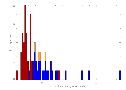
Figure 1: Histogram of the critical radii of lenses for the various samples considered in this work: sample A1 (brown and orange); Bolton et al. (2006) SLACS sample of 28 lenses (19 confirmed lenses and 9 candidates) (blue). Note that the SLACS lenses have systematically larger critical radii as a consequence of their spectroscopic selection from the SDSS.

Finally, we add the SLACS lenses (Bolton et al. 2006) to construct our largest sample comprising seventy systems. The SLACS survey has proven to be a very efficient HST Snapshot imaging survey for new galaxy-scale strong lenses. The targeted lens candidates were selected by Bolton et al. (2006) from the SDSS database of galaxy spectra for having multiple nebular emission lines at a redshift significantly higher than that of the target SDSS galaxy. The survey is optimized to detect bright early-type lens galaxies with faint lensed sources. The key advantage of this selection technique is that it provides a homogeneously selected sample of bright early-type lens galaxies. However, given the size of the fibres in SDSS this sample is biased toward large separations (the consequences of this bias are discussed later) compared to other surveys. This is clearly seen in the histogram plotted in Fig. 1. All the 28 SLACS lenses found to date are tabulated in Table A2 of the Appendix. Of these lenses 19 are confirmed with multiple images and the remaining 9 lenses are candidates. We note here that both the confirmed and unconfirmed candidates from the SLACS are included in our calculations. Although the SLACS is a biased sample, we include all 28 lenses in our analysis to illustrate the effect of better statistics given the success of the adopted selection strategy. The SLACS selection favours gravitational lenses that have typically larger Einstein radii (as seen clearly in the histogram of image separations in Fig. 1) by virtue of the selection of spectroscopic candidates for imaging follow-up. For the purposes of the current analysis it clearly strengthens the results of this work, i.e. biased sampling of the image separation distribution provides biased values for galaxy evolution parameters. Once the survey has finished, the selection function will be very well determined, which will enable more careful use of this sample for galaxy evolution studies. This strategy has been extremely successful so we feel compelled to showcase this sample. SLACS E/S0 lenses appear to be a random sub-sample of the luminous red galaxies sample of the SDSS, only skewed toward the brighter and higher surface brightness systems. While the environments of some of the lenses are complicated by the existence of nearby galaxies, by and large it is a ‘clean’ sample where the image separations are determined primarily by a single elliptical/S0 lens. Including the 28 SLACS lenses to the sample A1 gives us a final tally of 70 lenses, all with complete information, that defines our sample A2. In Fig. 1, we plot the distribution of critical radii for observed lenses in sample A1 and the SLACS lenses, which together constitute our sample A2. Since several samples will be used in the paper, we list them here for clarity: Sample A1 - our updated version of the ORM sample I, with a total of 42 systems; Sample A2 - our new, enlarged sample that contains Sample A1 and 28 new SLACS lenses; Sample B - our mock sample of a 100 lenses with complete information; and Sample C: our truncated sample A1 with 10% of the largest separation lenses removed.

4 Analysis and results

In this section, we compare the discriminating power of the MVDF versus the IVDF, in constraining both cosmological and galaxy evolution parameters. We study the recovery bias in the extraction of (i) cosmological constraints with $U=P=0$ for the various compiled lens samples, as well as of (ii) galaxy evolution parameters, by fixing the cosmological parameters. Finally, we assess the impact of incompleteness of lens data in the recovery of the cosmological constant.

As noted in section 2, we normalise the lens-redshift probability distribution with respect to the optical depth $\tau$. Therefore, parameters which appear simply as multiplying constants in the distributions do not impact our comparison. Such parameters include the Hubble radius $r_{H}=c/H_{0}$ and the average number density of lensing galaxies $n_{\star}$ (IVDF) and ${n_{\star}}^{\prime}$ (MVDF). Our comparison of the IVDF and MVDF is not affected by the value of $f_{E}$. This parameter relates the velocity dispersion of the dark matter to that of the stars. TOG set it to $(3/2)^{1/2}$, other studies (e.g. Narayan & Bartelmann 1999) suggested using values smaller than 1. Recent results from the SLACS survey suggest that $f_{E}\sim 1$, i.e. the lens model velocity dispersions are fairly close to the measured stellar velocity dispersion within an effective radius (Treu et al. 2006). Therefore, we take $f_{E}=1$ in this work. The default cosmological model is taken to be a Friedmann-Robertson-Walker ($\Omega_{\Lambda}+\Omega_{M}+\Omega_{K}=1$) $\Lambda$-CDM flat Universe, with $\Omega_{M}=0.3$, $\Omega_{K}=0.0$ and $\Omega_{\Lambda}=0.7$.

The parameters that affect our analysis are the ones defining the VDFs: $\sigma_{\star}$, $\gamma$, $\alpha$, $\sigma_{\star}^{\prime}$, $\alpha^{\prime}$, $\beta^{\prime}$. For the IVDF: $\alpha$ is the faint-end slope in the Schechter luminosity function, and $\gamma$ is the Faber-Jackson power-law index. For the MVDF: $\alpha^{\prime}$ is the low-velocity power-law index, and $\beta^{\prime}$ is the high-velocity exponential cutoff index of the distribution. Following ORM, the values $(n_{\star\rm{E}},n_{\star\rm{S0}},\sigma_{\star},\alpha,\gamma)$ = ($0.0039h^{3}\hbox{Mpc}^{-3}$, $0.0061h^{3}\hbox{Mpc}^{-3}$, $225\hbox{ km s}^{-1}$, -0.54, 4) are used for the IVDF. Following MKFS fit to the MVDF, we take $({n_{\star}}^{\prime},\sigma_{\star}^{\prime},\alpha^{\prime},\beta^{\prime})$ = ($0.0041h^{3}\hbox{Mpc}^{-3}$, $88.8\hbox{ km s}^{-1}$, 6.5, 1.93).

Note that late-type galaxies can in principle also be incorporated into the IVDF analysis easily, by simply replacing the Faber-Jackson relation with the Tully-Fisher relation. We can substitute the Faber-Jackson exponent $\gamma$ and characteristic $\sigma_{\star}$ with the corresponding Tully-Fisher relation parameters. Although late-type galaxies are more numerous than early-type galaxies, they tend to have lower masses and therefore do not contribute significantly to the total optical depth to lensing. Due to the strong dependence of the lensing cross section on the velocity dispersion, this causes late-type galaxies in general to be inefficient lenses. Besides, late-type galaxies are not included in the determination of the MVDF from SDSS data. So in this work, for consistent comparisons we restrict ourselves to elliptical and S0 lenses.

We compute the differential optical depth $(d\tau/dz)/\tau$ for each individual lens with measured separation and known source redshift for our two samples: sample A1 (42 lenses) and sample A2 (70 lenses). We then determine the probability distribution of the redshift of the lens using equation (7) (IVDF) and equation (13) (MVDF), given the observed image separation; the measured source redshift; a given cosmology and galaxy evolution model (in this case assuming no evolution: $U=P=Q=0$, $h=0.7$, $\Omega_{M}=0.3$, $\Omega_{K}=0.0$ and $\Omega_{\Lambda}=0.7$). If the choice of underlying cosmological parameters, primarily $\Omega_{\Lambda}$ in this case, corresponds to the true value, the peak of the probability distribution $z_{p}$ ought to be close to the measured lens redshift $z_{l}$, in a good number of cases. These lens redshift probability distributions are shown in Fig. A2 (in the Appendix) for all the lenses in our sample A2. The plot illustrates that the MVDF and IVDF yield near identical probability distributions for the lens redshifts. Choosing different values of $\Omega_{\Lambda}$ shifts these inferred probability distributions: this is illustrated in Fig. 2 for one lens (B0218+357), for values of $\Omega_{\Lambda}=0.2,0.4,0.7\hbox{ and }1.0$ (keeping $\Omega_{K}=0.0$). However, we notice a systematic effect: $z_{p}$ the peak redshift of the probability distribution is skewed slightly lower for the MVDF compared to the IVDF for almost the entire sample A2. This can be qualitatively explained as arising due to the different asymptotic behaviours of the MVDF and the IVDF (see Fig. A1 in the Appendix).

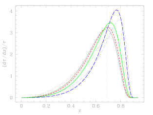
Figure 2: Dependence of the lens-redshift distribution on cosmology. We show the dependence on the value of $\Omega_{\Lambda}$ explicitly for the lens B0218+357 using the MVDF (thick lines) and IVDF (thin lines) respectively, for a range of values: $\Omega_{\Lambda}=0.2$ (black, dotted), $\Omega_{\Lambda}=0.4$ (red, short-dashed), $\Omega_{\Lambda}=0.7$ (green, solid) and $\Omega_{\Lambda}=1.0$ (blue, long-dashed). The vertical dashed line marks the position of the observed lens redshift $z_{l}=0.69$. The peak $z_{p}$ of the distribution increases as $\Omega_{\Lambda}$ increases from 0.2 to 1.0, due to the increase in the cosmological comoving volume.

4.1 The maximum likelihood method

Now, we use the samples to statistically play the game in both directions: (i) constrain the geometry of the Universe with galaxy evolution parameters fixed, and (ii) to constrain the galaxy evolution model with cosmological parameters as knowns.

We use a maximum likelihood estimator in our statistical analysis of lens redshift distributions. The lens-redshift test equations give the probability distribution of lens redshifts as $P(z_{l}|\{X\},z_{s},r)$, normalised to unity, where $\{X\}=\{\Omega_{\Lambda},U,P\}$ is the set of cosmological and galaxy evolution model parameters, and $(z_{s},r)$ are source redshift and lens angular critical radius priors for a given system. The likelihood estimator $L$ for the entire sample of $N$ systems is then:

$$L(\{X\})=\prod_{i=1}^{N}P_{i}(z_{l}|\{X\},z_{s},r).$$ (15)

The quantity $L$ is computed to quantify the consistency of all measured lens redshifts for the entire ensemble of lens systems for any given geometry and galaxy evolution model.

We then compute the maximum value of $L$, fixing the galaxy evolution parameters to obtain constraints on the cosmology ($\{X\}=\{\Omega_{\Lambda}\}$), and then fixing the cosmology to obtain constraints on galaxy evolution ($\{X\}=\{U,P\}$).

As pointed out by ORM, the lens-redshift test is more sensitive to the galaxy mass evolution parameter $U$ compared to the galaxy number evolution parameter $P$. This can be understood by considering the limit when $P\sim 0$: a negative $U$ decreases the most probable value for the lens redshift and narrows the probability distribution. In contrast, the number evolution parameter only affects the peak value but does not affect the overall shape of the probability distribution.

4.1.1 Constraints on cosmology

We proceed to obtain constraints on $\Omega_{\Lambda}$, keeping galaxy evolution parameters fixed, using the Friedmann-Robertson-Walker cosmology, and imposing $\Omega_{\Lambda}+\Omega_{M}+\Omega_{K}=1$ with $\Omega_{K}=0.0$. Unless otherwise stated, we assume $U=P=Q=0$, corresponding to the case of no evolution in the galaxy population either in mass or number. The lens-redshift test equations (7) and (13) are used in this instance and the likelihood as described above is constructed and maximized.

A projection of the likelihood surface along the $\Omega_{\Lambda}$ axis for sample A1 is shown in Fig. 3. In the upper panel the likelihood function is calculated using the IVDF for sample A1. Several values of $\sigma_{\star}$ are shown for completeness. Assuming a value of $\sigma_{\star}=225\hbox{ km s}^{-1}$ for elliptical galaxies (ORM), we obtain the following limits on the cosmological constant: $\Omega_{\Lambda}=0.55_{-0.20}^{+0.14}$ at $1\sigma$ confidence. This value is determined by taking the median as the central value and ”ruling out” the leftmost $\sim 16$% and rightmost $\sim 16$% of the total integral (‘median’ method). Alternatively, if we take the mode as the central value and determine the threshold value of the likelihood for which the integral under it comprises $\sim 68$% of the total integral (‘mode’ method), we obtain a slightly higher value of $\Omega_{\Lambda}=0.60_{-0.19}^{+0.13}$; this method is similar to what ORM did, except that they assumed a normal distribution (‘normal’ method). Their assumption turns out to be quite reasonable as we recover the same results ($\Omega_{\Lambda}=0.60_{-0.18}^{+0.12}$) applying their method to our sample A1. For the IVDF, we note that the error bars we obtain are much smaller than in ORM: this is certainly due to the larger number of lens systems in our sample A1 (the ORM sample I had 15 lenses compared to 42 in our sample A1). Although our error bars are smaller, we note that the numbers quoted here are for a single value of $\sigma_{\star}=225\hbox{ km s}^{-1}$ and these determinations of $\Omega_{\Lambda}$ using the ‘mode’, ‘median’ and ‘normal’ methods are entirely consistent with each other within the errors.

The corresponding results for sample A1 using the MVDF are also shown in Fig. 3 (lower panel): in this case as well, several values of $\sigma_{\star}^{\prime}$ are plotted to present the trend clearly. Assuming $\sigma_{\star}^{\prime}=88.8\hbox{ km s}^{-1}$ (Sheth et al. 2003, MKFS), we obtain a value for the cosmological constant of $\Omega_{\Lambda}=0.62_{-0.17}^{+0.12}$ using the ‘median’ method, $\Omega_{\Lambda}=0.67_{-0.16}^{+0.11}$ using the ‘mode’ method, and $\Omega_{\Lambda}=0.67_{-0.15}^{+0.11}$ using the ‘normal’ method. Again, we note that these quoted values are for a single value of $\sigma_{\star}^{\prime}=88.8\hbox{ km s}^{-1}$ and once again the constraints on $\Omega_{\Lambda}$ using these three different criteria are consistent with each other given the errors. Even with the improvement of using the MVDF compared to earlier work, the sensitivity to $\Omega_{\Lambda}$ in the lens-redshift test is low, as seen clearly by the fact that using the $\pm 1\sigma$ range on $\sigma_{\star}^{\prime}$ recovers values of $\Omega_{\Lambda}$ varying from 0.0 to nearly 1.0 - the full available range.

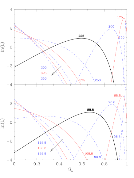
Figure 3: The projection of the likelihood surface along the $\Omega_{\Lambda}$ axis is shown here for several values of the characteristic velocity dispersion $\sigma_{\star}$ (IVDF; upper panel) and $\sigma_{\star}^{\prime}$ (MVDF; lower panel) for sample A1. The numbers denote the characteristic velocity dispersion in $\hbox{ km s}^{-1}$, increasing in value from the top down in both panels as indicated by the arrows. For $\sigma_{\star}=225\hbox{ km s}^{-1}$ (black thick line, upper panel), we obtain $\Omega_{\Lambda}=0.60_{-0.19}^{+0.13}$. For $\sigma_{\star}^{\prime}=88.8\hbox{ km s}^{-1}$ (black thick line, lower panel), we obtain $\Omega_{\Lambda}=0.67_{-0.16}^{+0.11}$. The likelihood curves are very shallow and consequently the error bars are rather large. The MVDF and IVDF constraints on $\Omega_{\Lambda}$ are in good agreement.

Unsurprisingly, the recovery of $\Omega_{\Lambda}$ using the MVDF and the IVDF yields very similar values, as these functions differ only at the extremely high ($\sigma_{\star}>380\hbox{ km s}^{-1}$) velocity dispersion tail as shown in Fig. A1 in the Appendix. A marked difference between the IVDF and MVDF shows up in the velocity range of 380–400 $\hbox{ km s}^{-1}$, which is characteristic of cD galaxies. Strong lensing events from such galaxies are difficult to model, as their position at the centre of clusters causes the events to be assisted by additional smoothly distributed dark matter in their vicinity. Since we excluded all such systems in our sample A1, it is not surprising that the inferred value of the cosmological constant using the IVDF and MVDF are in good agreement.

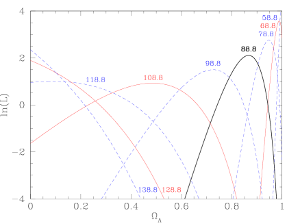
Figure 4: The projection of the likelihood surface along the $\Omega_{\Lambda}$ axis is shown here for several values of the characteristic velocity dispersion $\sigma_{\star}^{\prime}$ for the full sample A2 using the MVDF. The numbers denote the characteristic velocity dispersion in $\hbox{ km s}^{-1}$, increasing in value from the top down as indicated by the arrows. For For $\sigma_{\star}^{\prime}=88.8\hbox{ km s}^{-1}$ (black thick line), we obtain $\Omega_{\Lambda}=0.87_{-0.06}^{+0.04}$. The likelihood curves are very shallow and consequently the error bars are rather large. The sample A2 clearly yields values of $\Omega_{\Lambda}$ that are systematically higher than sample A1.

We plot the corresponding results for the larger sample A2 in Fig. 4 employing the MVDF. Once again we plot the projection of the likelihood for various values of $\sigma_{\star}^{\prime}$. For $\sigma_{\star}^{\prime}=88.8\hbox{ km s}^{-1}$, we now find $\Omega_{\Lambda}=0.86_{-0.06}^{+0.04}$ for the ‘median’ method; $\Omega_{\Lambda}=0.87_{-0.06}^{+0.04}$ for the ‘mode’ method and $\Omega_{\Lambda}=0.87_{-0.06}^{+0.04}$ for the ‘normal’ method.

We find that the recovered value of $\Omega_{\Lambda}$ is higher from the sample A2 (the mode value is shifted by about 0.25). Sample A2 does include a higher proportion of larger separation lenses (clearly seen in Fig. 1). This indicates a potential systematic bias that skews recovery of $\Omega_{\Lambda}$, that is sensitive to how well the ‘true’ separation distribution is sampled. To obtain robust constraints on $\Omega_{\Lambda}$ with the lens-redshift test not only do we need large samples but we also need lenses that accurately reflect the true underlying distribution of image separations. We note here that the SLACS lenses are included to clearly demonstrate this bias as their image separations are skewed to larger values as a consequence of the selection technique.

Four key results emerge from these plots: first, the lens-redshift test is not very robust in constraining the value of the cosmological constant with current samples. This was already suggested by K92, but we demonstrate it more clearly here even with two notable improvements: a larger sample of lenses and the use of the MVDF. The likelihood curve is very shallow and consequently the error bars are rather large. Second, the MVDF and IVDF results are comparable, therefore the inefficacy of the lens-redshift test does not appear to stem from systematics arising from the use of the IVDF. Third, is the notable sensitivity of constraints on $\Omega_{\Lambda}$ to the parameter $\sigma^{{}^{\prime}}_{*}$. The value of $\sigma^{{}^{\prime}}_{*}$ emerges in the fit of a functional form to the observed velocity dispersion function and depends on the completeness of the measurement, i.e. adequate sampling of the high and low velocity dispersion tail for observed galaxies. Finally, inclusion of the SLACS lenses (19 confirmed lenses + 9 candidates) with relatively larger separations pushes the recovered $\Omega_{\Lambda}$ to higher values. The finite number of lens systems is clearly implicated here as evidenced in the error bars on $\Omega_{\Lambda}$ and is a key limitation. In conclusion, as we show in the next section, while a large number of lens systems will go a ways toward increasing the robustness of this test in the future, it is crucial to simultaneously sample the separation distribution uniformly.

4.1.2 Constraints on galaxy evolution

We now investigate galaxy evolution using the lens-redshift test, with $n_{\star}$, $L_{\star}$, $\sigma_{\star}$, $n_{\star}^{\prime}$, $L_{\star}^{\prime}$ and $\sigma_{\star}^{\prime}$ varying with redshift according to equations (8), (9) and (10) and their primed versions. The equations used are (11) and (14). Fixing the cosmological model to $h=0.7$, $\Omega_{M}=0.3$, $\Omega_{K}=0.0$ and $\Omega_{\Lambda}=0.7$, we determine $U$ and $P$. As outlined in Section 4.1, the likelihood function is constructed fixing $\Omega_{\Lambda}$ and then maximizing to obtain constraints on $U$ and $P$.

We obtain constraints on $U$ and $P$ for various samples: the ORM sample I lenses, sample A1 and sample A2 all of which are plotted in Fig. 5. We calculate the $U$-$P$ contours for the ORM sample I, applying our analysis methods and using the MVDF. The MVDF was not available at the time of the ORM analysis. Our calculation of the $U$ and $P$ parameters using the IVDF is in very good agreement with their results. The orientation and calibration of the confidence level contours agree. Although the contours of all the samples overlap quite well, the difference in the peak values of $U$ and $P$ determined for our samples A1, A2 and ORM sample I is significant.

The likelihood results in the $U$-$P$ plane for sample A1, using the IVDF and the MVDF, are shown in the upper and the lower panels of Fig. 5, respectively. We obtain a maximum in $L$ at {$U=0.11$, $P=-1.40$} for the IVDF and at {$U=0.10$, $P=-1.24$} for the MVDF, again showing no significant dependence on the choice of velocity dispersion function employed. However, we note that the contours close along the $U$-axis for the MVDF case compared to the IVDF. Therefore, using the IVDF to calculate the likelihood lowers the sensitivity to mass evolution. For our sample A2 the maximum value for $L$ is at {$U=0.32$, $P=-1.60$} for the IVDF and at {$U=0.28$, $P=-1.57$} for the MVDF. For the ORM sample I: the maximum value for $L$ is found to lie at {$U=-0.08$, $P=0.44$} for the IVDF and at {$U=-0.07$, $P=0.85$} for the MVDF. The likelihood peak moves toward increasingly positive values of U for sample A2 compared to A1 and the ORM sample I. This indicates a strong sensitivity to the fraction of large separation lenses. Sample A2 has a larger proportion of those and therefore predicts stronger mass evolution for the lens ensemble.

The fact that $U$ and $P$ have opposite signs is consistent with mass conservation: we have either a larger number of lower mass galaxies ($P>0$, $U<0$) or fewer more massive galaxies ($P<0$, $U>0$) in the past compared to today. However, the case ($P<0$, $U>0$) is in conflict with the currently accepted hierarchical model of galaxy formation with bottom-up assembly of structure.

Our primary conclusions on deriving galaxy evolution parameters are: (i) we reproduce the trends reported by ORM for their sample I when we use the IVDF as they did; (ii) we find the likelihood peak position to be insensitive to the choice of IVDF vs MVDF for the ORM sample I; (iii) we recover $U$ and $P$ values consistent within the errors for all our samples; (iv) with a larger number of lenses (as in sample A2) we obtain slightly increased sensitivity to $P$ compared to ORM sample I; (v) the likelihood peak shifts systematically to higher $U$ values for sample A2 which contains a higher proportion of large separation lenses compared to the sample A1. To summarise, there is a notable observational bias in recovering mass evolution that depends strongly on how well the underlying true separation distribution is sampled in detected lenses.

4.1.3 Investigation of systematic observational biases

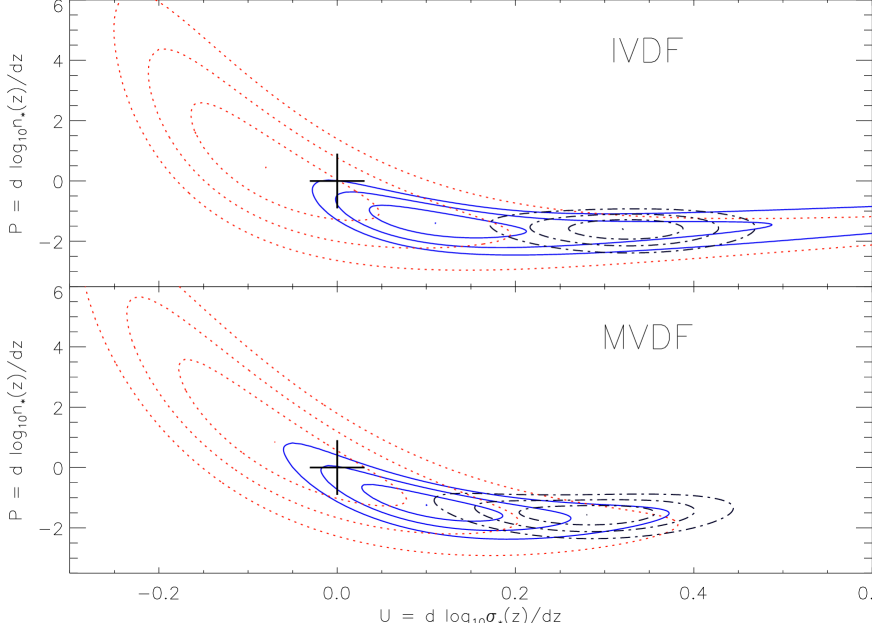
Figure 5: Comparison of constraints on galaxy evolution for different samples: the derived $U$-$P$ contours for sample A1 (blue, solid lines), sample A2 (black, dot-dashed lines) and the ORM sample I (red, dashed lines). In the upper panel, the IVDF was used for the calculation and in the lower panel the MVDF. The three contours shown for each sample are the $1\sigma$, $2\sigma$ and $3\sigma$ confidence levels and the cross marks the no-evolution locus $(U=0,P=0)$. While there is some degree of overlap for the various samples it is clear that the peak value of $U$ – the mass evolution parameter – shifts toward more positive values consistent with sample A2 having a larger proportion of more massive lenses, in good agreement with the fact that sample A2 does have a higher fraction of large separation lenses. The error bars on the ORM sample I are larger since it has only 15 systems whereas sample A1 has 42 systems and sample A2 70 systems. We note that within the errors the values of $U$ and $P$ obtained for different samples are in good agreement.

Unbiased lens surveys are needed to sample uniformly the full distribution of separations (Kochanek 1993) in order to apply the lens-redshift test to constrain galaxy evolution parameters as found above. If the sample is slightly skewed toward larger separations, biased values of the galaxy evolution parameters are retrieved. To investigate this issue further, we create a mock sample of a hundred lenses (sample B), all with complete information (i.e. source redshift, lens redshift, and image separation) known assuming no evolution, to try and understand the observational biases that likely affect our analysis. We randomly assign the source redshift from a normal distribution of redshifts centred at $z=2$ and with a dispersion of 1. We then randomly assign the angular critical radius, as half of the lens separation, from the probability distribution of image separations given by Kochanek (1993), where we set $\gamma=4$ and $\alpha=-1$ in their equation (4.10) for a flat Universe. We calculate the differential optical depth distribution for each lens, using equation (7), and randomly pick a lens redshift from it.

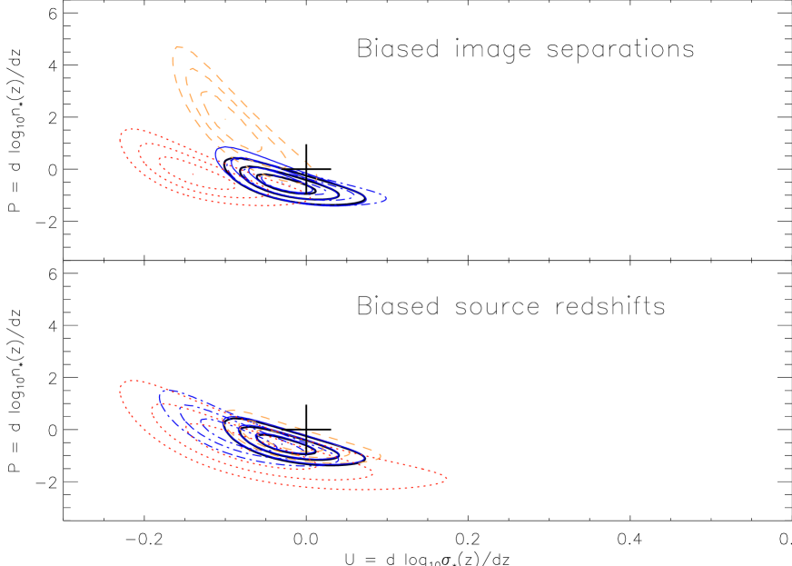
Figure 6: Effect of biased lens samples and the recovery of $U$ and $P$ illustrated for the IVDF case. Upper panel [Biased image separations]: $U$-$P$ contours for our full mock sample B and several subsamples selected by cuts in image separations (i) lowest $90\%$ separations (blue, dot-dashed thin lines), (ii) lowest $58\%$ separations (red, dotted thin lines), (iii) largest $90\%$ separations (blue, solid thin lines), (iv) largest $58\%$ separations (orange, dashed thin lines). Lower panel [Biased source redshifts]: $U$-$P$ contours for subsamples now cut on the basis of source redshifts (i) lowest $90\%$ $z_{s}$ (blue, dot-dashed thin lines), (ii) lowest $58\%$ $z_{s}$ (red, dotted thin lines), (iii) highest $90\%$ $z_{s}$ (blue, solid thin lines), (iv) highest $58\%$ $z_{s}$ (orange, dashed thin lines). The full mock sample B results (black, solid thick lines) are shown in both panels for comparison. The three contours shown for each sample are the $1\sigma$, $2\sigma$ and $3\sigma$ contour likelihood lines and the cross marks the location of the no-evolution locus $(U=0,P=0)$. A clear systematic bias is introduced on selection by lens separation. In particular, the velocity dispersion evolution parameter dramatically shifts from near-zero values ($U\sim 0$) to negative values ($U\sim-0.1$), when the largest separation lenses are removed from the sample.

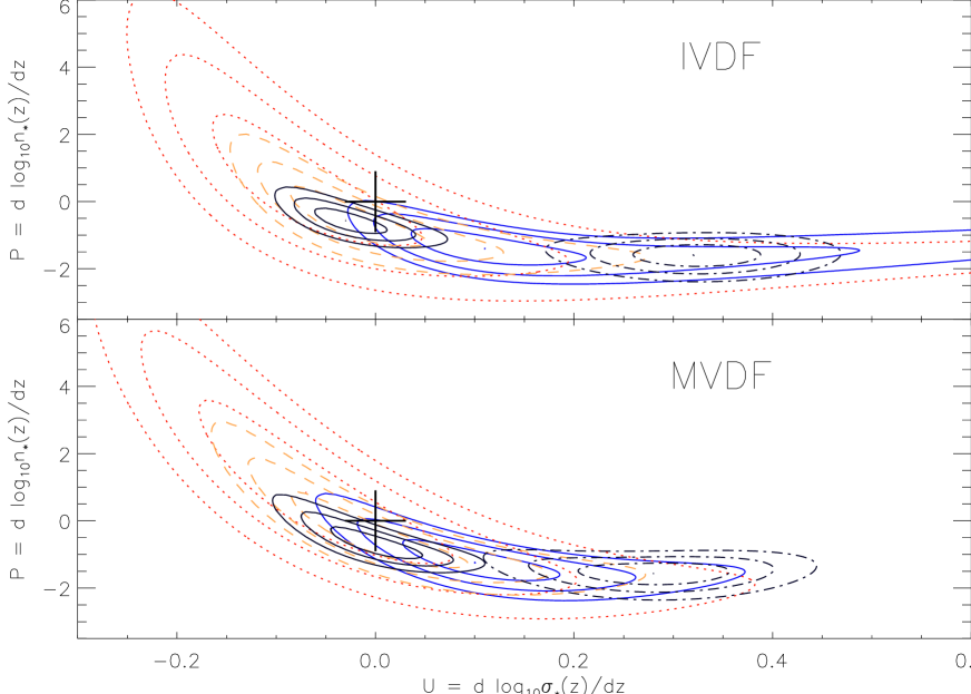
Figure 7: Illustrating the systematic bias arising from poorly sampling the true image separation distribution: the $U$-$P$ contours for ORM sample I (red, dotted lines) and our samples A1 (blue, solid lines), A2 (black, dot-dashed lines), C (orange, dashed lines), and B (black, solid lines) are shown for the IVDF (upper panel) and MVDF (lower panel). The three contours shown for each sample are the $1\sigma$, $2\sigma$ and $3\sigma$ confidence levels, with the cross marking $(U=0,P=0)$ denoting the no-evolution case. The systematic bias induced in our sample A2 arises from a larger fraction of large image separation lenses.

For the full mock catalogue (sample B), the maximum value for the likelihood $L$ is obtained at {$U=-0.03$, $P=-0.57$}. The input $(U=0,P=0)$ parameters values are not exactly recovered due to finite-sample variance. Several subsamples of sample B were then evaluated, after cutting the sample based on source redshifts and image separations. Creating a subsample of 90 lenses discarding the 10 highest source redshift systems, we find that the maximum value of the likelihood $L$ shifts to {$U=-0.09$, $P=-0.21$}. Then for a subsample of 90 lenses generated by discarding the 10 lowest source redshift systems we find that the peak is at {$U=-0.03$, $P=-0.54$}.

To examine the additional sensitivity to the number of lenses as well, we now construct a subsample from sample B of 58 lenses with the lowest source redshifts and find {$U=-0.07$, $P=-0.80$} and for the subsample of 58 lenses with the highest source redshifts the evolution parameters are found to be {$U=-0.02$, $P=-0.48$}. These results are shown in the lower panel of Fig. 6: no significant systematic bias is introduced on selection by source redshift. The only difference seen in these subsamples is the effect of the variation in the number of systems: the contours are more extended for the 2 cases with 58 systems compared to the cases with 90 systems.

We then cull sample B on the basis of image separations and the results for these subsamples are shown in the upper panel of Fig. 6. The key systematic that we study in further detail is the role of biased sampling of the image separation distribution. The mock catalogue generated above was now cut based on lens angular critical radius $r$. Once again biased subsamples were generated to preferentially sample larger and smaller separation systems. First, we constructed a subsample of 90 systems discarding 10 smallest separation systems: for this instance the maximum value of the likelihood lies at {$U=-0.03$, $P=-0.49$}. Picking now a further 90 systems discarding the 10 largest separation systems, we find a different maximum at {$U=-0.02$, $P=-0.62$}. Similarly, making a more extreme selection, we pick 58 systems from the mock discarding 42 of the largest separation systems. This is our extreme biased sample skewed to small separations. For this subsample we find {$U=-0.14$, $P=-0.19$}. Finally, for a mock with 58 of the largest separation lenses (this constitutes our extreme biased sample toward large separations) we find {$U=-0.10$, $P=1.92$}. Our analysis clearly indicates the presence of a systematic bias introduced on selection by lens separation. This effect is especially seen clearly in the smaller subsamples (with 58 systems). In particular, the velocity dispersion evolution parameter dramatically shifts from near-zero values ($U\sim 0$) to negative values ($U\sim-0.1$), when the highest separation lenses are removed from the sample. We see clearly from Fig. 6 that lens data comprising biased sampling of the underlying image separation distribution introduce a systematic shift in the recovered values of the galaxy evolution parameters, whereas data with biased source redshifts yield unbiased estimates of $U$ and $P$.

Galaxy evolution parameters are thus extremely sensitive to observational biases in the separation distribution of lens systems. For ground based optical surveys and high resolution HST surveys there are optimal separations that are detected. Lens systems found in ground based surveys are likely skewed to larger separations than those found in HST surveys.

Having narrowed the plausible source of the systematic bias, we re-do the analysis making a similar cut on our observed lens sample A1 to verify our finding. We remove the five (10%) largest image separation lenses thus creating the sample C. We now compare the recovery of $U$ and $P$ for this biased sample with samples A1 and A2, sample B and the ORM sample I. The maximum value of $L$ is obtained for sample C at {$U=-0.03$, $P=-0.51$} (IVDF) and at {$U=-0.01$, $P=-0.40$} (MVDF). In Table 1 we list the positions of the peak values of the likelihood function in the $U$-$P$ plane, for our samples A1, A2, B, ORM sample I and sample C, for the IVDF and MVDF. The full results are shown in Fig. 7. The resultant trend clearly demonstrates the strong bias now replicated with cuts in the data introduced by artificially removing large image separation systems. Our result that incompleteness in image separations is a serious current limitation in using strong lensing statistics has also been pointed out by Oguri (2005) and Oguri, Keeton & Dalal (2005).

Sample	U=$\hbox{d log}_{10}\sigma_{\star}(z)/dz$	P=$\hbox{d log}_{10}n_{\star}(z)/dz$
A2 (IVDF)	+0.32	-1.60
A1 (IVDF)	+0.11	-1.40
B (IVDF)	-0.03	-0.57
C (IVDF)	-0.03	-0.51
ORM I (IVDF)	-0.08	+0.44
A2 (MVDF)	+0.28	-1.57
A1 (MVDF)	+0.10	-1.24
B (MVDF)	+0.00	-0.71
C (MVDF)	-0.01	-0.40
ORM I (MVDF)	-0.07	+0.85

Table 1: Positions of the peak values of the likelihood function in the U-P plane, for samples A2, A1, B, C, and ORM I, IVDF and MVDF, in order of U-peak position. When comparing samples A2, A1 and C, we confirm the same trend we observed with the mock subsamples: the velocity dispersion evolution parameter shifts to less positive values as we remove the highest separation lenses.

5 The effect of incomplete lens data on the retrieval of cosmological parameters

Previous lens-redshift test analyses have differed on how to handle systems with incomplete redshift information. K96 included an estimate of the probability of failing to measure a system’s lens redshift for systems lacking such a measurement. ORM take a more pragmatic approach by discarding all systems with $z_{s}>2.1$, arguing that systems below that redshift are mostly complete. The former approach is made difficult by the many variables that can prevent a successful redshift measurement (surface brightness of the lensing galaxy, galaxy contrast with respect to the magnified source images, observing conditions during an actual measurement attempt), while the latter approach ignores higher-redshift systems that do have complete redshift information. Such systems are likely to show the strongest sensitivity to cosmological or evolution effects that are sought after in the first place.

The approach we adopt here is to marginalise over systems with incomplete redshift information using nested Monte Carlo simulations. Let $N_{c}$ be the number of systems with complete redshift information and $N_{u}$ be the number of systems with unmeasured lensing redshifts. For a given parameter set $\{X\}$, we can assign lens redshifts for the $N_{u}$ sample by drawing from $P(z_{l}|\{X\},z_{s},r)$ which gives a sample of lens redshifts $\{z_{l,u}\}$. With $\{z_{l,u}\}$ fixed, we obtain the absolute likelihood $L(\{X\})$ for the combined $N_{c}+N_{u}$ sample. The procedure is then repeated $N_{MC}$ times with each iteration using a different set of $\{z_{l,u}\}$. This gives an average absolute likelihood $<L(\{X\})>$ and a corresponding scatter $\delta L(\{X\})$ for the given set of model parameters $\{X\}$. The scatter in the absolute likelihood estimate shrinks to zero as $N_{u}\rightarrow 0$, and can be interpreted as a measure of the uncertainty in the absolute likelihood because of the incomplete sample. The entire procedure can then be repeated for a different set of model parameters.

We argue that this is an attractive method for several reasons. First, it does not ignore existing redshift information for any system, either within the complete or the incomplete sample. This results in as large a sample size as possible and helps to minimize small-number effects that are traditionally present in lensing statistics. Second, the question of handling biases present in the incomplete sample is made objectively by marginalising over the entire sample rather than imposing an artificial cut on, say, the source redshifts. And third, it allows one to quantify the effects that the incomplete sample has on the accuracy of likelihood analysis through $\delta L(\{X\})$. This last point can be used to explore how the precision of the model parameters can be measured by future changes in either the complete or incomplete sample size.

We performed a nested Monte Carlo simulation of our sample A1 ($N_{c}=42$), adding a set of ten mock lens systems with known image separations, source redshifts and unknown lens redshift ($N_{u}=10$), to make up a total of 52 lens systems. We fixed all galaxy evolution parameters ($U=P=Q=0$, $\sigma_{\star}=225\hbox{ km s}^{-1}$) and varied cosmological parameters, after setting $\Omega_{\Lambda}+\Omega_{M}+\Omega_{K}=1$ with $\Omega_{K}=0.0$. Therefore, the parameter set was taken to be $\{X\}=\{\Omega_{\Lambda}\}$. A projection of the (un-normalised) likelihood surface along the $\Omega_{\Lambda}$ axis is shown in Fig. 8 for the IVDF case: we show the results for $\Omega_{\Lambda}$ values steps of of 0.1 only, and for $N_{MC}=100$. The blue line is the result for the sample A1. For each fixed value of $\Omega_{\Lambda}$, each of the points represents the value of the likelihood for one of the $N_{MC}=100$ different possible sets of the combined $N_{c}+N_{u}$ sample. Approximating the likelihood distributions with Gaussian functions of mean $\mu=<L(\{X\})>$ and dispersion $\sigma=\delta L(\{X\})$, the average absolute likelihood $<L(\{X\})>$ for the combined $N_{c}+N_{u}$ sample follows the pattern given by the complete system (blue line), being almost flat between $\Omega_{\Lambda}=0.0$ and $\Omega_{\Lambda}=0.7$. Therefore adding even a small number of systems with incomplete information reduces further the sensitivity to $\Omega_{\Lambda}$.

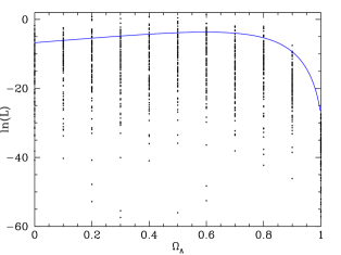
Figure 8: The projection of the (un-normalised) likelihood surface along the $\Omega_{\Lambda}$ axis is shown here for hundred independent realizations of 52 lens systems (IVDF case), comprising 42 systems from sample A1 and 10 mock systems. All galaxy evolution parameters being fixed ($U=P=Q=0$, $\sigma_{\star}=225\hbox{ km s}^{-1}$), each dot represents the value of the likelihood L for a particular value of $\Omega_{\Lambda}$ and for a particular set of 52 lenses. The blue line is the result for sample A1 (42 lenses) only. For each value of $\Omega_{\Lambda}$, the distribution of 100 likelihood values can be approximated by a Gaussian function with a mean $\mu=<L(\{X\})>$ and a dispersion $\sigma=\delta L(\{X\})$.

The effect of incomplete information is to further dilute the efficacy of constraints on cosmological parameters. While we have argued here that the lens-redshift test with a small lens sample with complete information is insufficient, we further find even with a small number of systems in a large sample with incomplete information, we lose sensitivity to $\Omega_{\Lambda}$.

6 Conclusions and Discussion

We investigate the lens-redshift test to assess its robustness in constraining cosmological and galaxy evolution parameters. We apply the test to a much improved lens sample compared to earlier work by K92 and ORM. Moreover, we also use the observationally determined velocity dispersion function (MVDF), instead of relying on the IVDF. MKFS also used the MVDF, but they applied it to the ODTL test, which is more affected by observational biases - mainly the magnification bias - than the lens-redshift test considered here. Finally, we develop a new nested Monte Carlo analysis to quantify the effects of incompleteness on the accuracy of retrieving $\Omega_{\Lambda}$.

Our results suggest that the lens-redshift test is not particularly robust in the determination of either cosmological parameters or galaxy evolution parameters with the currently available samples. We conclude this after careful analysis of 70 lens systems and generating several mock catalogues. First, we fix galaxy evolution parameters to constrain $\Omega_{\Lambda}$: in this instance very weak constraints are obtained. Moreover, despite using the MVDF for the first time in this test our results do not differ significantly from earlier work. When we do the converse, i.e. fix the cosmology and look for constraints on galaxy evolution, we find that the results on the evolution parameters are too sensitive to the choice of sample, implying a very strong dependence on the observational bias introduced by lens separations. Finally, the limit of the precision with which the value of the cosmological constant can be determined due to lack of complete information has been assessed. We find that even a small number of systems with incomplete information in a large sample can further reduce the significance of the already weak constraints on the cosmological constant. In fact, systems with incomplete information add more noise than signal. For the purposes of constraining cosmological parameters incomplete-redshift information systems are best excluded. With the small number of systems available at the present time, such a strong cut is not feasible, however with the expected large number of new lenses from future surveys the statistics will permit stricter selection of optimal systems.

The lens-redshift test is clearly affected by lens selection effects. An obvious observational strategy for the future would be to observe hundreds of new lenses, that fairly sample the full distribution of separations. Such samples are expected from the large area surveys to be performed by future instruments like SNAP and the LSST. These large samples with hundreds/thousands of lenses at several redshifts would allow us to better quantify the lens sample selection bias. Moreover, ideally lenses for use in the lens-redshift test need to be relatively “clean”, that is, they should not belong to groups, where presence of additional deflectors/nearby galaxies could affect the image separation and therefore provide skewed lens image separation distributions that will in turn bias results. It is becoming increasingly clear from the study of individual lens environments that there are clearly no truly isolated lenses. However, what is important from the point of view of the lens-redshift test is that the neighbouring perturbers are not massive enough to significantly alter the image separations to within observational positional accuracies. Obviously these accuracies depend on whether space based data or ground based data is available for new lens systems. From large proposed future surveys which all involve deep imaging, lens systems with many perturbers need to be culled. It appears from simulations that systems that likely require of the order of 10 - 20% external shear are still viable candidates for the lens-redshift test (Oguri, Keeton & Dalal 2005) .

Future lens samples should ideally include both early and late type galaxies and span a large redshift range, in order to constrain galaxy evolution parameters. Finally, all lens systems to be useful should have complete information, since even a small fraction of incomplete systems would significantly decrease the efficacy of constraints on parameters. In the near future, hundreds/thousands of new lens systems will be discovered by these upcoming new instruments. Simultaneously with many on-going and planned ambitious surveys to study galaxy evolution, progress is likely to come from better knowledge of galaxy evolution. The lens-redshift test, which is currently unable to give decent constraints on cosmology and galaxy evolution because of poor statistics, could eventually prove to be a very profitable means to constrain cosmological parameters and galaxy evolution models robustly.

Appendix A Tables and additional figures

Number	Name	R.A.	Dec.	$z_{s}$	$z_{l}$	$r$	Grade	$N_{im}$	Samples	References
(1)	(2)	(3)	(4)	(5)	(6)	(7)	(8)	(9)	(10)	(11)
1	HE0047-1756	00:50:27.83	$-$17:40:8.8	$1.67$	$0.41$	$0.773$	A	2	A1,C,O	1,2
2	Q0142-100	01:45:16.5	$-$09:45:17	$2.72$	$0.49$	$1.205$	A	2	A1,C,O	3,45
3	QJ0158-4325	01:58:41.44	$-$43:25:04.20	$1.29$	$0.28$	$0.615$	A	2	A1,C,O	3,4
4	HE0435-1223	04:38:14.9	$-$12:17:14.4	$1.69$	$0.46$	$1.208$	A	4	A1,C,O	2,5,47
5	HS0818+1227	08:21:39.1	$+$12:17:29	$3.12$	$0.39$	$1.199$	A	2	A1,C,O	6
6	SDSS0903+5028	09:03:34.92	$+$50:28:19.2	$3.61$	$0.39$	$1.451$	A	2	A1,O	7
7	RXJ0911+0551	09:11:27:50	$+$05:50:52.0	$2.80$	$0.77$	$1.104$	A	4	A1,C,O	8,9
8	SBS0909+523	09:13:01.05	$+$52:59:28.83	$1.38$	$0.83$	$0.534$	A	2	A1,C,I,O	10
9	SDSS0924+0219	09:24:55.87	$+$02:19:24.9	$1.52$	$0.39$	$0.866$	A	4	A1,C,O	2,11
10	FBQ0951+2635	09:51:22.57	$+$26:35:14.1	$1.24$	$0.26$	$0.541$	A	2	A1,C,I,O	3,12,45
11	BRI0952-0115	09:55:00.01	$-$01:30:05.0	$4.50$	$0.63$	$0.525$	A	2	A1,C,O	2,3,13,45
12	J1004+1229	10:04:24.9	$+$12:29:22.3	$2.65$	$0.95$	$0.770$	A	2	A1,C,O	14
13	LBQS1009-0252	10:12:15.71	$-$03:07:02.0	$2.74$	$0.87$	$0.779$	A	2	A1,C,O	2,15,46
14	Q1017-207	10:17:24.13	$-$20:47:00.4	$2.55$	$0.86$	$0.461$	A	2	A1,C,O	2,3,16
15	FSC10214+4724	10:24:34.6	$+$47:09:11	$2.29$	$0.96$	$0.820$	A	2E	A1,C,O	3,17
16	HE1104-1805	11:06:33.45	$-$18:21:24.2	$2.32$	$0.73$	$1.724$	A	2	A1,O	18
17	PG1115+080	11:18:17.00	$+$07:45:57.7	$1.72$	$0.31$	$1.144$	A	4	A1,C,I,O	19,20
18	RXJ1131-1231	11:31:51.6	$-$12:31:57	$0.66$	$0.30$	$1.817$	A	4	A1,O	21
19	SDSS1138+0314	11:38:03.70	$+$03:14:58.0	$2.44$	$0.45$	$0.664$	A	4	A1,C,O	22,23
20	SDSS1155+6346	11:55:17:35	$+$63:46:22.0	$2.89$	$0.18$	$0.897$	A	2	A1,C,O	22
21	SDSS1226-0006	12:26:08.10	$-$00:06:02.0	$1.12$	$0.52$	$0.634$	A	2	A1,C,O	23
22	SDSS1335+0118	13:35:34.79	$+$01:18:05.5	$1.57$	$0.44$	$0.780$	A	2	A1,C,O	23
23	Q1355-2257	13:55:43.38	$-$22:57:22.9	$1.37$	$0.70$	$0.646$	A	2	A1,C,O	2,45
24	SBS1520+530	15:21:44.83	$+$52:54:48.6	$1.86$	$0.72$	$0.743$	A	2	A1,C,I,O	24
25	WFI2033-4723	20:33:42.08	$-$47:23:43.0	$1.66$	$0.66$	$0.980$	A	4	A1,C,O	2
26	HE2149-2745	21:52:07.44	$-$27:31:50.2	$2.03$	$0.60$	$0.857$	A	2	A1,C,I,O	25,26,45
27	B0218+357	02:21:05.483	$+$35:56:13.78	$0.94$	$0.69$	$0.169$	A	2ER	A1,C,I,R	27,28
28	MG0414+0534	04:14:37.73	$+$05:34:44.3	$2.64$	$0.96$	$1.187$	A	4E	A1,C,R	29,30
20	B0712+472	07:16:03.58	$+$47:08:50.0	$1.34$	$0.41$	$0.716$	A	4	A1,C,I,R	31
30	MG0751+2716	07:51:41.46	$+$27:16:31.35	$3.20$	$0.35$	$0.402$	A	R	A1,C,R	30
31	B1030+074	10:33:34.08	$+$07:11:25.5	$1.54$	$0.60$	$0.514$	A	2	A1,C,I,R	31
32	B1152+200	11:55:18.3	$+$19:39:42.2	$1.02$	$0.44$	$0.807$	A	2	A1,C,I,R	32
33	B1422+231	14:24:38.09	$+$22:56:00.6	$3.62$	$0.34$	$0.779$	A	4E	A1,C,R	20,33
34	MG1549+3047	15:49:12.37	$+$30:47:16.6	$1.17$	$0.11$	$1.150$	A	R	A1,C,I,R	34,35
35	PMN1632-0033	16:32:57.68	$-$00:33:21.1	$3.42$	$1.17$	$0.731$	B	2R	A1,C,R	2,36
36	MG1654+1346	16:54:41.83	$+$13:46:22.0	$1.74$	$0.25$	$0.982$	A	R	A1,C,I,R	37
37	PKS1830-211	18:33:39.94	$-$21:03:39.7	$2.51$	$0.89$	$0.471$	A	2ER	A1,C,R	38
38	B1933+503	19:34:30.95	$+$50:25:23.6	$2.62$	$0.76$	$0.506$	A	2R	A1,C,R	49
39	Q0047-2808	00:49:41.89	$-$27:52:25.7	$3.60$	$0.48$	$1.163$	A	4ER	A1,C,M	40
40	HST14113+5211	14:11:19.60	$+$52:11:29.0	$2.81$	$0.47$	$2.260$	A	4	A1,M	9,10
41	HST14176+5226	14:17:36.61	$+$52:26:40.0	$3.40$	$0.81$	$3.250$	A	4	A1,M	41
42	HST15433+5352	15:43:20.9	$+$53:51:52	$2.09$	$0.50$	$1.176$	A	2R	A1,C,M	41
43	HE0512-3329	05:14:10.78	$-$33:26:22.50	$1.57$	$0.93$	$0.322$	A	2	I	42
44	B1600+434	16:01:40.45	$+$43:16:47.8	$1.59$	$0.41$	$0.690$	A	2	I	31
45	B1608+656	16:09:13.96	$+$65:32:29.0	$1.39$	$0.63$	$1.135$	A	4	I	43
46	FBQ1633+3134	16:33:48.99	$+$31:34:11.90	$1.52$	$0.68$	$0.330$	B	2	I	44

Table 2: The columns are: (1) lens number; (2) lens name; (3) R.A. [h:m:s], J2000.0; (4) Dec. [d:m:s], J2000.0; (5) source redshift, $z_{s}$; (6) lens redshift, $z_{l}$; (7) critical radius, $r$, in arcseconds; (8) grade for the likelihood that the object is a lens: A=I’d bet my life, B=I’d bet your life, and C=I’d bet your life and you should worry (CASTLES); (9) Number of images corresponding to each source component, E means extended and R means there is an Einstein ring (CASTLES); (10) sample: A1- Sample A1 in this paper, C- Sample C in this paper, I- Sample I in ORM, O- Targeted optical discoveries, R- Targeted radio discoveries, M- Miscellaneous discoveries; (11) references. The numbers shown are the ones actually used in the computations. When computing ORM Sample I, we used the numbers from ORM Table A1 (calculating the critical radius, $r$, as half of the separation).
List of references:
$1$ - Wisotzki et al. (2004); $2$ - Ofek et al. (2006); $3$ - Rusin et al. (2003); $4$ - Morgan et al. (1999); $5$ - Wisotzki et al. (2002); $6$ - Hagen & Reimers (2000); $7$ - Johnston et al.(2003); $8$ - Kneib, Cohen & Hjorth (2000); $9$ - Kochanek et al. (2000); $10$ - Lubin et al. (2000); $11$ - Eigenbrod et al. (2006a); $12$ - Schechter et al. (1998); $13$ - Lehar et al. (2000); $14$ - Lacy et al. (2002); $15$ - Hewett et al. (1994); $16$ - Surdej et al. (1997); $17$ - Eisenhardt et al. (1996); $18$ - Lidman et al. (2000); $19$ - Weymann et al. (1980); $20$ - Tonry (1998); $21$ - Sluse et al. (2003); $22$ - Oguri et al. (2005); $23$ - Eigenbrod et al. (2006b); $24$ - Burud et al. (2002a); $25$ - Wisotzki et al. (1996); $26$ - Burud et al. (2002b); $27$ - Cohen, Lawrence & Blandford (2003); $28$ - Wiklind & Combes (1995); $29$ - Lawrence et al. (1995); $30$ - Tonry & Kochanek (1999); $31$ - Fassnacht & Cohen (1998); $32$ - Myers et al. (1999); $33$ - Patnaik et al. (1992); $34$ - Lehar et al. (1993); $35$ - Treu & Koopmans (2003); $36$ - Winn et al. (2002); $37$ - Langston et al. (1989); $38$ - Wiklind & Combes (1996); $39$ - Sykes et al. (1998); $40$ - Warren et al. (1996); $41$ - Ratnatunga et al. (1998); $42$ - Gregg et al. (2000); $43$ - Fassnacht et al. (1996); $44$ - Morgan et al. (2001); $45$ - Eigenbrod et al. (2007); $46$ - Surdej et al. (1993); $47$ - Morgan et al. (2005).

Number	Name	$z_{s}$	$z_{l}$	$\sigma_{a}$	Status
(1)	(2)	(3)	(4)	(5)	(6)
1	SDSS J003753.21$-$094220.1	0.632	0.195	$265\pm 10$	C
2	SDSS J021652.54$-$081345.3	0.524	0.332	$332\pm 23$	C
3	SDSS J073728.45$+$321618.5	0.581	0.322	$310\pm 15$	C
4	SDSS J081931.92$+$453444.8	0.446	0.194	$231\pm 16$	UC
5	SDSS J091205.30$+$002901.1	0.324	0.164	$313\pm 12$	C
6	SDSS J095320.42$+$520543.7	0.467	0.131	$207\pm 14$	UC
7	SDSS J095629.77$+$510006.6	0.470	0.241	$299\pm 16$	C
8	SDSS J095944.07$+$041017.0	0.535	0.126	$212\pm 12$	C
9	SDSS J102551.31$-$003517.4	0.276	0.159	$247\pm 11$	C
10	SDSS J111739.60$+$053413.9	0.823	0.229	$279\pm 21$	UC
11	SDSS J120540.43$+$491029.3	0.481	0.215	$235\pm 10$	UC
12	SDSS J125028.25$+$052349.0	0.795	0.232	$254\pm 14$	C
13	SDSS J125135.70$-$020805.1	0.784	0.224	$216\pm 23$	C
14	SDSS J125919.05$+$613408.6	0.449	0.233	$263\pm 17$	UC
15	SDSS J133045.53$-$014841.6	0.712	0.081	$178\pm 09$	C
16	SDSS J140228.21$+$632133.5	0.481	0.205	$275\pm 15$	C
17	SDSS J142015.85$+$601914.8	0.535	0.063	$194\pm 05$	C
18	SDSS J154731.22$+$572000.0	0.396	0.188	$243\pm 11$	UC
19	SDSS J161843.10$+$435327.4	0.666	0.199	$257\pm 25$	C
20	SDSS J162746.44$-$005357.5	0.524	0.208	$275\pm 12$	C
21	SDSS J163028.15$+$452036.2	0.793	0.248	$260\pm 16$	C
22	SDSS J163602.61$+$470729.5	0.675	0.228	$221\pm 15$	UC
23	SDSS J170216.76$+$332044.7	0.436	0.178	$239\pm 14$	UC
24	SDSS J171837.39$+$642452.2	0.737	0.090	$270\pm 16$	C
25	SDSS J230053.14$+$002237.9	0.464	0.229	$283\pm 18$	C
26	SDSS J230321.72$+$142217.9	0.517	0.155	$260\pm 15$	C
27	SDSS J232120.93$-$093910.2	0.532	0.082	$236\pm 07$	C
28	SDSS J234728.08$-$000521.2	0.715	0.417	$330\pm 50$	UC

Table 3: List of all lenses belonging to Bolton et al. (2006) sample. The columns are: (1) lens number; (2) lens name; (3) source redshift, $z_{s}$; (4) lens redshift, $z_{l}$; (5) velocity dispersion measured within an aperture $\sigma_{a}$, in $\hbox{ km s}^{-1}$ and (6) the status of the lens (C - confirmed; UC - unconfirmed). The numbers shown are the ones actually used in the computations (only the central value of $\sigma_{a}$ was used). The critical radius $r$ was then computed using equation (2) and $h=0.7$, $\Omega_{\Lambda}=0.7$, $\Omega_{M}=0.3$, and $\Omega_{K}=0.0$. Note that the 19 confirmed lenses and 9 candidates are denoted with a $C$ and $UC$ respectively in the final column.

Figure 9: The measured velocity dispersion function (MVDF) and the inferred velocity dispersion function (IVDF) for early-type galaxies. The functional forms plotted here are derived from fits provided in equation (23) of Mitchell et al. (2005). The solid curve is the MVDF and the dashed curve is the IVDF.

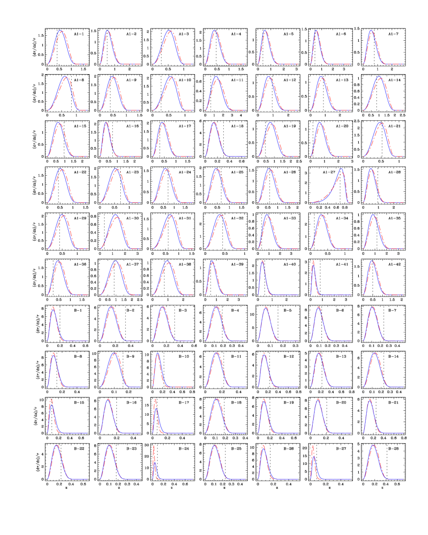
Figure 10: The lens-redshift distribution (${(d\tau/dz)}/\tau$ vs $z$) for all 70 lenses from Sample A1 (numbered in the same order as presented in Table A1 in the Appendix) and the Bolton at al. (2006) SLACS sample (numbered in the same order as presented in Table A2 in the Appendix): calculated using the IVDF (red, dot-dashed line) and the MVDF (blue, solid line); with the galaxy evolution and cosmological parameters set to $U=P=Q=0$, $h=0.7$, $\Omega_{\Lambda}=0.7$, $\Omega_{M}=0.3$, and $\Omega_{K}=0.0$. The vertical dashed line marks the position of the observed lens redshift $z_{l}$. The peak $z_{p}$ of the probability distribution is skewed to slightly higher $z_{l}$ for the IVDF compared to the MVDF, in most lenses.

References

- [Augusto et al. (2001)] Augusto P. et al., 2001, MNRAS, 326, 1007
- [Barkana et al.(1999)] Barkana R., Blandford R. D., Hogg D. W., 1999, ApJ, 513, L91
- [Bennett et al.(1986)] Bennett C. L., Lawrence C. R., Burke B. F., Hewitt J. N., Mahoney J., 1986, ApJS, 61, 1
- [Blandford & Narayan(1992)] Blandford R. D., Narayan R., 1992, ARA&A, 30, 311
- [Bolton et al.(2006)] Bolton A. S., Burles S., Koopmans L. V. E., Treu T., Moustakas L. A., 2006, ApJ, 638, 703
- [Burud et al.(2002)] Burud I., et al., 2002, A&A, 383, 71
- [Burud et al.(2002)] Burud I. et al., 2002, A&A, 391, 481
- [Chae et al.(2002)] Chae K.-H.et al., 2002, Physical Review Letters, 89, 151301
- [Chae(2003)] Chae K.-H., 2003, MNRAS, 346, 746
- [Cheng & Krauss(1998)] Cheng Y.-C. N., Krauss L. M., 1998, preprint (astro-ph/9810393)
- [Cohen et al.(2003)] Cohen J. G., Lawrence C. R., Blandford R. D., 2003, ApJ, 583, 67
- [Colless et al.(2001)] Colless M. et al., 2001, MNRAS, 328, 1039
- [Crampton et al. (2002)] Crampton D. et al., 2002, ApJ, 570, 86
- [Eigenbrod et al.(2006)] Eigenbrod A., Courbin F., Dye S., Meylan G., Sluse D., Vuissoz C., Magain P., 2006, A&A, 451, 747
- [Eigenbrod et al.(2006)] Eigenbrod A., Courbin F., Meylan G., Vuissoz C., Magain P., 2006, A&A, 451, 759
- [Eigenbrod et al.(2007)] Eigenbrod A., Courbin F., Meylan G., 2007, A&A, 465, 51
- [Eisenhardt et al.(1996)] Eisenhardt P. R., Armus L., Hogg D. W., Soifer B. T., Neugebauer G., Werner M. W., 1996, ApJ, 461, 72
- [Fassnacht et al.(1996)] Fassnach C. D., Womble D. S., Neugebauer G., Browne I. W. A., Readhead A. C. S., Matthews K., Pearson T. J., 1996, ApJL, 460, L103
- [Fassnacht & Cohen(1998)] Fassnacht C. D., Cohen J. G., 1998, AJ, 115, 377
- [Gregg et al.(2000)] Gregg M. D., Wisotzki L., Becker R. H., Maza J., Schechter P. L., White R. L., Brotherton M. S., Winn J. N., 2000, AJ, 119, 2535
- [Hagen & Reimers(2000)] Hagen H.-J., Reimers D., 2000, A&A, 357, L29
- [Hewett et al.(1994)] Hewett P. C., Irwin M. J., Foltz C. B., Harding M. E., Corrigan R. T., Webster R. L., Dinshaw N., 1994, AJ, 108, 1534
- [Huchra et al. (1985)] Huchra et al., 1985, AJ, 90, 691
- [Johnston et al.(2003)] Johnston D. E. et al., 2003, AJ, 126, 2281
- [Keeton 2001] Keeton C., 2001, preprint (astro-ph/0102340)
- [Kneib et al.(2000)] Kneib J.-P., Cohen J. G., Hjorth J. 2000, ApJL, 544, L35
- [Kochanek(1992)] Kochanek C. S., 1992, ApJ, 384, 1
- [Kochanek(1993)] Kochanek C. S., 1993, ApJ, 419, 12
- [Kochanek(1996)] Kochanek C. S., 1996, ApJ, 466, 638
- [Kochanek et al.(2000)] Kochanek C. S. et al., 2000, ApJ, 543, 131
- [Kochanek(2004)] Kochanek C. S., 2004, preprint (astro-ph/0407232)
- [Lacy et al.(2002)] Lacy M., Gregg M., Becker R. H., White R. L., Glikman E., Helfand D., Winn J. N., 2002, AJ, 123, 2925
- [Langston et al.(1989)] Langston G. I. et al., 1989, AJ, 97, 1283
- [Lawrence et al.(1995)] Lawrence C. R., Elston R., Januzzi B. T., Turner E. L., 1995, AJ, 110, 2570
- [Lehar et al.(1993)] Lehar J., Langston G. I., Silber A., Lawrence C. R., Burke B. F., 1993, AJ, 105, 847
- [Lehar et al.(2000)] Lehar J. et al., 2000, ApJ, 536, 584
- [Lidman et al.(2000)] Lidman C., Courbin F., Kneib J.-P., Golse G., Castander F., Soucail G., 2000, A&A, 364, L62
- [Lubin et al.(2000)] Lubin L. M., Fassnacht C. D., Readhead A. C. S., Blandford R. D., Kundić, T., 2000, AJ, 119, 451
- [Maoz 2005] Maoz D., 2005, preprint (astro-ph/0501491)
- [Maoz & Rix(1993)] Maoz D., Rix H.-W., 1993, ApJ, 416, 425
- [Maoz et al.(1993)] Maoz D. et al., 1993, ApJ, 409, 28
- [Maza et al.(1996)] Maza J., Wischnjewsky M., Antezana R., 1996, Revista Mexicana de Astronomia y Astrofisica, 32, 35
- [Mitchell et al.(2005)] Mitchell J. L., Keeton C. R., Frieman J. A., Sheth R. K., 2005, ApJ, 622, 81
- [Morgan et al.(1999)] Morgan N. D., Dressler A., Maza J., Schechter P. L., Winn J. N., 1999, AJ, 118, 1444
- [Morgan et al.(2001)] Morgan N. D., Becker R. H., Gregg M. D., Schechter P. L., White R. L., 2001, AJ, 121, 611
- [Morgan et al.(2005)] Morgan N. D., Kochanek C. S., Pevunova O., Schechter P. L., 2005, AJ, 129, 2531
- [Muñoz et al.(1998)] Muñoz J. A., Falco E. E., Kochanek C. S., Lehár J., McLeod B. A., Impey C. D., Rix H.-W., Peng C. Y., 1998, Ap&SS, 263, 51
- [Myers et al.(1999)] Myers S. T. et al., 1999, AJ, 117, 2565
- [Myers et al.(2003)] Myers S. T. et al., 2003, MNRAS, 341, 1
- [Narayan & Bartelmann(1996)] Narayan R., Bartelmann M., 1996, preprint (astro-ph/9606001)
- [Narayan & Bartelmann(1999)] Narayan R., Bartelmann M., 1999, Formation of Structure in the Universe, 360
- [Ofek et al.(2003)] Ofek E. O., Rix H.-W., Maoz D., 2003, MNRAS, 343, 639
- [Ofek et al.(2006)] Ofek E. O., Maoz D., Rix H.-W., Kochanek C. S., Falco E. E., 2006, ApJ, 641, 70
- [Oguri (2005)] Oguri M., 2005, MNRAS, 361, L38
- [Oguri et al.(2005)] Oguri M. et al., 2005, ApJ, 622, 106
- [Oguri, Keeton & Dalal (2005)] Oguri M., Keeton C., Dalal N., 2006, MNRAS, 364, 1451
- [Ostriker & Steinhardt(1995)] Ostriker J. P., Steinhardt P. J., 1995, Nature, 377, 600
- [Patnaik et al.(1992)] Patnaik A. R., Browne I. W. A., Walsh D., Chaffee F. H., Foltz C. B., 1992, MNRAS, 259, 1P
- [Perlmutter et al.(1999)] Perlmutter S. et al., 1999, ApJ, 517, 565
- [Ratnatunga et al.(1999)] Ratnatunga K. U., Griffiths R. E., Ostrander E. J., 1999, AJ, 117, 2010
- [Riess et al.(1998)] Riess A. G. et al., 1998, AJ, 116, 1009
- [Rusin et al.(2003)] Rusin D., Kochanek C. S., Keeton C. R., 2003, ApJ, 595, 29
- [Saha & Williams(2003)] Saha P., Williams L. L. R., 2003, AJ, 125, 2769
- [Schechter et al.(1998)] Schechter P. L., Gregg M. D., Becker R. H., Helfand D. J., White R. L., 1998, AJ, 115, 1371
- [Sheth et al.(2003)] Sheth R. K. et al., 2003, ApJ, 594, 225
- [Sluse et al.(2003)] Sluse D., et al., 2003, A&A, 406, L43
- [Spergel et al.(2006)] Spergel D. N. et al., 2006, preprint (astro-ph/0603449)
- [Surdej et al.(1993)] Surdej J., Remy M., Smette A., Claeskens J.-F., Magain P., Refsdal S., Swings J.-P., Veron-Cetty M., 1993, Proc. of the 31st Liege International Astrophysical Colloquium ”Gravitational lenses in the universe”, 31, 153-160
- [Surdej et al.(1997)] Surdej J., Claeskens J.-F., Remy M., Refsdal S., Pirenne B., Prieto A., Vanderriest C., 1997, A&A, 327, L1
- [Sykes et al.(1998)] Sykes C. M., et al., 1998, MNRAS, 301, 310
- [Tonry(1998)] Tonry J. L., 1998, AJ, 115, 1
- [Tonry & Kochanek(1999)] Tonry J. L., Kochanek C. S., 1999, AJ, 117, 2034
- [Treu & Koopmans(2003)] Treu T., Koopmans L. V. E., 2003, MNRAS, 343, L29
- [Treu et al. (2006)] Treu T., Koopmans L., Bolton A., Burles S. Moustakas L., 2006, ApJ, 640, 662
- [Turner et al.(1984)] Turner E. L., Ostriker J. P., Gott J. R., 1984, ApJ, 284, 1
- [Walsh et al.(1979)] Walsh D., Carswell R. F., Weymann R. J., 1979, Nature, 279, 381
- [Warren et al.(1996)] Warren S. J., Hewett P. C., Lewis G. F., Moller P., Iovino A., Shaver P. A., 1996, MNRAS, 278, 139
- [Weymann et al.(1980)] Weymann R. J. et al., 1980, Nature, 285, 641
- [Wiklind & Combes(1995)] Wiklind T., Combes F., 1995, A&A, 299, 382
- [Wiklind & Combes(1996)] Wiklind T., & Combe, F., 1996, Nature, 379, 139
- [Winn et al.(2002)] Winn J. N. et al., 2002, AJ, 123, 10
- [Wisotzki et al.(1996)] Wisotzki L., Koehler T., Lopez S., Reimers D., 1996, A&A, 315, L405
- [Wisotzki et al.(1998)] Wisotzki L., Wucknit, O., Lopez S., Sorensen A. N., 1998, A&A, 339, L73
- [Wisotzki et al.(2000)] Wisotzki L., Christlieb N., Bade N., Beckmann V., Köhler T., Vanelle C., Reimers D., 2000, A&A, 358, 77
- [Wisotzki et al.(2002)] Wisotzki L., Schechter P. L., Bradt H. V., Heinmüller J., Reimers D., 2002, A&A, 395, 17
- [Wisotzki et al.(2004)] Wisotzki L., Schechter P. L., Chen H.-W., Richstone D., Jahnke K., Sánchez S. F., Reimers D., 2004, A&A, 419, L31
- [York et al.(2000)] York D. G. et al., 2000, AJ, 120, 1579
- [Young et al. (1980)] Young P., Gunn J., Westphal J., Kristian J., 1980, ApJ, 241, 507