A competitive multi-agent model of interbank payment systems

Abstract

We develop a dynamic multi-agent model of an interbank payment system where banks choose their level of available funds on the basis of private payoff maximisation. The model consists of the repetition of a simultaneous move stage game with incomplete information, incomplete monitoring, and stochastic payoffs. Adaptation takes place with bayesian updating, with banks maximizing immediate payoffs. We carry out numerical simulations to solve the model and investigate two special scenarios: an operational incident and exogenous throughput guidelines for payment submission. We find that the demand for intraday credit is an S-shaped function of the cost ratio between intraday credit costs and the costs associated with delaying payments. We also find that the demand for liquidity is increased both under operational incidents and in the presence of effective throughput guidelines.

$\dagger$ Bank of England. E-mail: Marco.Galbiati@bankofengland.co.uk. The views expressed in this paper are those of the authors, and not necessarily those of the Bank of England.

$\ddagger$ Helsinki Univ. of Technology. E-mail: kimmo@soramaki.net.

The authors thank W. Beyeler, M. Manning, S. Millard, M. Willison for important insights. Useful comments came from the participants of a number of seminars: FS seminar (Bank of England, May 3, 2007), Central Bank Policy Workshop (Basel, March 13, 2007), University of Liverpool, Seimnar at the Computer Science Department (Liverpool, April 24, 2007). The usual disclaimer applies.

1 Introduction

Virtually all economic activity is facilitated by transfers of claims towards public or private financial institutions. The settlement of claims between banks takes to a large extent place at the central bank, in central bank money. These interbank payment systems transfer vast amounts of funds, and their smooth operation is critical for the functioning of the whole financial system. In 2004, the annual value of interbank payments made in the European TARGET was around $552 trillion, in the US Fedwire system $470 trillion, and in the UK CHAPS $59 trillion - tens of times the value of their respective gross domestic products (BIS 2006). These transfers originate from customer requests, and from the banks’ proprietary operations in e.g. foreign exchange, securities and the interbank money market. The sheer size of these transfers, and their centrality for the functioning of a number of markets, make the mechanisms that regulate these fluxes and the incentives that generate them interesting to policy makers and regulators.

At present most payment systems work on a real-time gross settlement (RTGS) or equivalent modality. In RTGS payments are settled continuously and individually throughout the day with immediate finality. To cover the payments banks generally use their reserve balances, access intraday credit from the central bank or use incoming funds from payments from other banks. The first two sources carry an (opportunity) cost which gives banks incentives to economize on their use. We call these funds liquidity. The third source, on the other hand, is dependent by the liquidity decisions of other banks. The less liquidity a bank commits for settlement, the more dependent it is from incoming payments - and may thus need to delay its own payments until these funds arrive, causing the receivers of its payments to receive funds later. If also delays are costly, each bank faces a trade-off between liquidity costs and delay costs. Both aspects are dependent on the banks own liquidity decision, but the latter is also dependent on the liquidity decisions by other banks.

This paper develops a dynamic model to study this trade-off. The model consists of a sequence of independent settlement days where a set of homogenous banks make payments to each other. Each of these days is a simultaneous-move game (or a stage game) in which banks choose their level of liquidity for payment processing. At the end of the day they receive a stochastic payoff determined by the amount of liquidity they committed and delays they experienced. Due to the nature of the settlement process, the payoff function is a random variable unknown to the banks. In this context, a reasonable assumption is that banks use heuristic, bounded-rational like rules to adapt their behaviour over time. Hence, we simulate a learning process taking place over many days, until banks settle down in equilibria. We are interested in the properties of the equilibria in aggregate terms, i.e. in the behaviour of the system as the product of independent, single agents’ private payoff maximization.

Given its game-theoretic approach, this paper is related to recent work by Angelini (1998), Bech and Garratt (2003, 2006), Buckle and Campbell (2003) and Willison (2004). These study various ”liquidity management games” with few (typically, two) agents and few (typically, three) periods. There, however, the payoff function is common knowledge. Due to the complex mechanics taking place in real payment systems this is likely to be unrealistic. Recent work by Beyeler et al. (2007) on the relationship between instruction arrival and payment settlement in a similar setting shows that with low liquidity, payment settlement gets coupled across the network and is governed by the dynamics of the queue - and largely unpredictable when a large number of payments are made. The present paper makes an effort to model this complexity; in a similar spirit, it also considers a large number of banks, which settle payments in a continuous-time day, and which interact over a long sequence of settlement days.

Recently, a growing literature has used simulation techniques to investigate the effects e.g. of failures in complex payment systems (see eg. BoE (2004), Leinonen (2005), Devriese and Mitchell (2005)). These studies generally use historical payment data and simulate banks’ risk exposures under alternative scenarios, or ways to improve liquidity efficiency of the systems. The shortcoming of this approach has been that the behaviour of banks is not endogenously determined. It is either assumed to remain unchanged or to change in a predetermined manner.

The present paper tries to overcome some of the shortcomings of both ”game theoretic” and ”simulation” approaches by modelling banks as learning agents. Agents who learn about each others’ actions through repeated interaction is a recurring theme in evolutionary game theory. In one strand of the literature the agents know their payoff function, and learn about others’ behaviour. They do so playing the stage game repeatedly, while choosing their actions on the basis of adaptive rules of the type ”choose a best reply to the current strategy profile” or ”choose a best reply to the next expected strategy profile”. Results obtained in this strand cannot be immediately applied here: banks cannot choose best replies as they do not know their payoff function. A second research line does not require knowledge of the payoff function on the part of the learners; they are instead of the kind ”adopt more frequently an action that has produced a high payoff in the past”. The main results of this literature are about the convergence (or non-convergence) of actions to equilibria of the stage game.

The approach adopted here is close to the latter. However, because the payoffs are calculated on the basis of a settlement algorithm, we cannot analytically calculate the equilibria ex-ante, and then demonstrate convergence (or the lack of it). Instead, we show convergence by means of simulations, inferring then that the attraction points are equilibria of the stage game - in a sense that we make precise. Because the payoff function is stochastic and unknown, the problem of each optimizing bank lends itself to a heuristic approach. From this perspective, our work bears strong links to the reinforcement learning literature. From an individual agent’s perspective it relates it relates to operations research, where a typical problem is that of maximizing an unknown function. However, in our setting the environment is not static: through time, actions yield different payoffs both because the payoff function is random, and because the other agents change their behaviour.

The model is rich enough to investigate a number of policy issues; here, we focus on the aggregate liquidity of the system. As a first result we derive a liquidity demand function, relating total funds to the ratio of delay to liquidity costs. This function is found to be increasing to the relative cost of delay, and S-shaped. Then, we look at the effect of operational incidents affecting random participants of the system. We find that banks would generally prefer to commit more liquidity in case the disruption were known - except from the extreme cases of very low and very high delay costs. Throughput guidelines for payment submission are a common used by system-designers to reduce risk in payment systems; we look at the effect of one such rule on liquidity usage and find that at sufficiently low delay costs banks would increase their liquidity holdings to contain delays. Finally, we explore some efficiency issues, namely whether smaller systems are more or less liquidity efficient than large ones. We find that a system with a smaller number of banks uses less liquidity for a given level of payment activity.

The paper is organised as follows: Section 2 develops a formal description of the model and the agents’ learning process, and describes the payoff function. Section 3 presents the results of the experiments and section 4 concludes.

2 Description of the model

2.1 Stage game and its repetition

The model consists of $N\$agents indexed by $i=1...N$, who repeatedly play a stage game $\Gamma=\left\langle A,\pi_{1},\pi_{2},...\pi_{N}\right\rangle$. Here $A=\left\{0,1,...K\right\}$ is the (common) finite action set for each agent, and $\pi_{i}:A^{N}\rightarrow\mathcal{F}$ is $i$’s outcome function, which maps the set of action profiles into a set of payoff distribution functions. That is, given the action profile $a\in A^{N}$, agent $i$ receives a stage-game payoff drawn from a univariate distribution $\pi_{i}\left(a\right)$, whose shape depends on $N$ parameters - the stage game action profile. To keep the exposition uncluttered, we leave the precise form of the outcome function $\pi_{i}\left(.\right)$ undefined at the stage. Details are given in Section 3.1, where we also give a precise economic interpretation to the abstract entities introduced here. Information in the game is incomplete as the outcome function $\pi\left(.\right)$ is unknown to the agents. Agents are risk-neutral, so they care about the expected payoff. Hence, bank $i$ will only be concerned with its payoff functions $f_{i}\left(a\right)=E\left(\pi_{i}\left(a\right)\right)$.

The stage game $\Gamma$ is repeated through discrete time, running from $t=0$ to (potentially) infinity. The action profile chosen in stage game $t$ is denoted by $a\left(t\right)=\left\{a_{1}\left(t\right),a_{2}\left(t\right),...,a_{N}\left(t\right)\right\}$. A particular realization of the payoff vector drawn from $\pi\left(a\left(t\right)\right)$, is indicated by $y\left(t\right)\in\mathbb{R}^{N}$, which is therefore also called the ”game-$t$ payoff”.

Monitoring is incomplete. At the beginning of (stage-) game $t$, each agent $i$ knows the following: all its own previous choices and realized payoffs, and some statistics of other’s past choices $\overline{a}_{-i}\left(k\right)$. A (observed) history (by $i$ at time $t$) is thus denoted by $h_{i}^{t}=\left\{a_{i}\left(k\right),y_{i}\left(k\right),\overline{a}_{-i}\left(k\right)\right\}_{k=0..t-1}$. Let us call $H^{t}$ the set of all possible histories that $i$ may observe up to $t$, and let us define $H=\cup H^{t}$. Differently from the literature on repeated games, but more in line with that on evolutionary game theory, we assume that agents aim at maximizing immediate payoffs (instead of e.g. the discounted stream of payoffs). That is, histories are essential to learn about payoffs and about others’ actions, but agents disregard strategic spillover effects between stage games. This seems a sensible assumption here: the complexity of the environment makes it unlikely that agents anticipate all interactions.

2.2 Information, learning and strategies

Agent $i$ faces two forms of uncertainty: uncertainty about the payoff function given others’ actions, and uncertainty about other’s actions. The first element gives to our model a flavour of decision theory, the second one is a game theory issue.

2.2.1 Information

As time goes by and histories are updated, agents can be seen to accumulate information. More formally, we posit that of the whole history observed up to $t$ each $i$ retains some multi-dimensional statistics, say $\wp_{i}\left(t\right)$. These are the beliefs about the state of the environment that $i$ is learning, and it constitutes the basis for the definition of strategies. Here, $\wp_{i}\left(t\right)$ is composed of two parts:

a) an ”estimate” $\widetilde{f}_{i}^{t}\left(.\right)$ of the payoff function $f_{i}\left(a\right)=$ $E\left[y_{i}\left|a\right.\right]$;

b) an ”estimate” $\widetilde{p}_{i}^{t}\left(.\right)$ of probabilities for other agents’ actions in the next stage game.

Of a whole action profile $a$, $i$ only observes its own action $a_{i}$ and a statistic $\overline{a}_{-i}$ which correlates with $a_{-i}.$ Hence, we assume that the estimate $\widetilde{f}_{i}^{t}\left(.\right)$ assigns to each $\left(a_{i},\overline{a}_{-i}\right)$ an expected payoff. As for the estimate b), each $i$ is assumed to maintain static expectations about others’ actions. That is, $i$ believes that $\overline{a}_{-i}$ is drawn from a time-invariant distribution, as if other agents were adopting a constant mixed strategy. We adopt this assumption, a classic in evolutionary game theory, because it is simple and because it yielded the same results as some more sophisticated forms of beliefs. Because action profiles that generate the same statistic $\overline{a}_{-i}$ are indistinguishable to $i$, the estimate $\widetilde{p}_{i}^{t}\left(.\right)$ also refers to $\overline{a}_{-i}$ instead of $a_{i}$. In the simulation, we posit that $\overline{a}_{-i}$ is the average action of the ”other” agents, which clearly takes values in $\left[0,K\right]$. So, approximating to the nearest integer, $\widetilde{p}_{i}^{t}\left(\overline{a}_{-i}\right)$ is a vector with $K$ entries, collecting the probabilities of any of the (other agents’) average action being played.

2.2.2 Learning

The information stored in $\widetilde{f}_{i}^{t}\left(.\right)$ and $\widetilde{p}_{i}^{t}\left(.\right)$ is updated as time goes by, according to learning rules. A learning rule for agent $i$, denoted by $\Lambda_{i}$, assigns to each observed history $h_{i}^{t-1}$ an updated $\wp_{i}\left(t\right)$.

Define $I_{k}\left(a_{i},\overline{a}_{-i}\right)$ as the indicator function equal to $1$ if action profile $\left(a_{i},\overline{a}_{-i}\right)$ appears at time $k$ and zero otherwise. We use the following learning rule:

$$\widetilde{f}_{i}^{t}\left(a_{i},\overline{a}_{-i}\right) =\frac{\sum_{k=0...t-1}y_{i}\left(k\right)I_{k}\left(a_{i},\overline{a}_{-i}\right)}{\sum_{k=0...t-1}I_{k}\left(a_{i},\overline{a}_{-i}\right)}$$ (1)

$$\widetilde{p}_{i}^{t}\left(\overline{a}_{-i}\right) =\frac{1+\sum_{k=1...t-1}I_{k}\left(\overline{a}_{-i}\right)}{t+K}$$ (2)

In words, $\widetilde{f}_{i}^{t}\left(a_{i},\overline{a}_{-i}\right)$ is the average payoff obtained under action profile $\left(a_{i},\overline{a}_{-i}\right)$ up until time $t$ excluded. Similarly, the components of the vector $\widetilde{p}_{i}^{t}\left(\overline{a}_{-i}\right)$ are calculated according to the observed frequencies, starting from an initial estimate $1/N$. This is known as the ”fictitious play” updating rule starting from a uniform estimate; it corresponds to Bayesian updating of beliefs about a constant, unknown distribution over the other agents’ actions.

2.2.3 Strategies

A strategy for $i$ is a map assigning to each $\wp_{i}(t)$ an action to be taken, i.e. some $a_{i}\left(t\right)$. A particular strategy can be seen as motivated by some ”rationale”, resting in turn on the basis of a learning process which we now describe.

Each $i$ is risk-neutral and aims at maximizing the expected immediate payoff. Because $i$ believes that the opponents play a particular $\overline{a}_{-i}$ with probability $\widetilde{p}_{i}^{t}\left(\overline{a}_{-i}\right)$, its strategy dictates:

$$a_{i}\left(t+1\right) =\arg\max_{a_{i}}E\left[\widetilde{f}_{i}^{t}\left(a_{i},\overline{a}_{-i}\right)\left|\widetilde{p}_{i}^{t}\right.\right]$$

$$=\arg\max_{a_{i}}\sum_{\overline{a}_{-i}}\widetilde{f}_{i}^{t}\left(a_{i},\overline{a}_{-i}\right)\widetilde{p}_{i}^{t}\left(\overline{a}_{-i}\right)\text{}$$ (3)

The fact that banks maximize their immediate payoff is only one of the many possible preference specifications. Alternatively, agents might also be taking into consideration future payoffs. In this case, however, optimal strategies would be far more complex. Indeed, discounting expected future payoffs would create an implicit trade-off between exploitation (the use of actions that appear optimal in the light of the available information), and exploration (the use of seemingly sub-optimal actions, which might appear such because of lack of experimentation). Our preference specification severs this payoff-related link between stage games, which nevertheless are interrelated because learning takes place across them. This short-sighted maximization assumption is common in the bounded-rationality and evolutionary game theory literature.

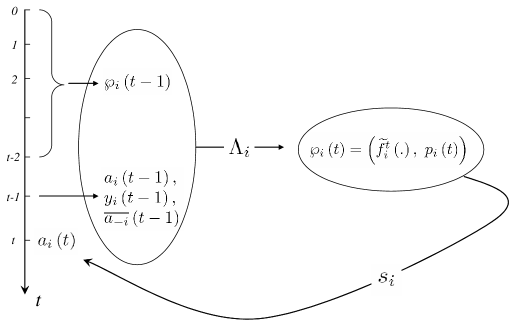
Figure 1: Information, learning and strategies

Figure 1 illustrates the relationship between histories, information and strategies. A history up to $t-2$ is summarized in $\wp_{i}(t-1)$. This, along with the new data obtained in $t-1$, is updated into $\wp_{i}\left(t\right)$ by the learning rule $\Lambda_{i}$. In turn $\wp_{i}\left(t\right)$, which is the information available at $t$, is mapped by a strategy $s_{i}$, to an action $a_{i}\left(t\right)$.

It should be noted that in early repetitions of the stage game, $\widetilde{p}_{i}^{t}$ is heavily influenced by the initial (arbitrary) estimate, for which we simply use $1/K$, while $\widetilde{f}_{i}^{t}\left(.\right)$ is the average of a few observed payoffs only. Hence, strict adoption of Eq. 3 would most likely yield, and possibly lock into, sub-optimal actions. To avoid this, we suppose that agents first randomly choose a certain number of actions to explore the environment, and then start making choices as in Eq. 3 - which we call ”informed decisions”. To ensure further exploration, each agent also tries itself out at least once every $\overline{a}_{-i}$ that it encounters. This models learning from other agents.

These choices on the length of the ”exploration phase” are evidently arbitrary; however, in the model there are clearly no exploration costs, so the length of the exploration period can indeed be assumed exogenously. On the other hand, some limit to exploration must be imposed, as the sheer size of the action spaces inhibits a brute force approach, whereby $i$ collects a very large sample of all possible action profiles (and respective payoffs) before making informed decisions.

2.3 Specification of the payoff function

The model of learning about an unknown stochastic payoff function that is determined party by the agent’s own actions and partly by the actions of other agents can lend itself to a number of applications. The specification of the payoff function $f_{i}$ ties it to the problem of a payment system analyzed in this paper.

One possible specification of $f$  could be a simple analytical function of the players’ actions. The problem would then become that of analyzing the limiting behaviour of the learning rules and strategies, something that could be done analytically, provided $f$ is simple enough. However, in quest of increased realism in payment system modelling we specify $f$ via an algorithm representing a ”settlement day” with a large number of daily payments. To understand why realistic analytical functions are difficult to develop, consider the following: imagine first that banks have always enough liquidity to make payments instantaneously. In this case payments flow undisturbed, delay costs are zero, and only liquidity costs matter. Their calculation is trivial. However, if banks commit less funds for settlement (as banks want to minimize costs), it becomes more likely that the funds are at some point insufficient for banks to execute payments immediately. As shown in Beyeler et al.. (2006), these liquidity shortages cause payments to occur in ”cascades”, whose length and frequency bears no correlation with the instruction arrival process that regulates payment instructions as the settlement of payments becomes coupled across the network when incoming funds allow the bank to release previously queued payment. As a consequence, the flow of liquidity and thus delay times for individual banks become largely unpredictable.

In the model $a_{i}$ represents any external funding decision by the bank. The funds allow the bank to execute payment instructions, which the bank receives throughout the day according to a random process. Banks have costs for both committing liquidity for settlement, and from experiencing delays in payment processing due to insufficient funds. The settlement day is modelled in continuous time, with time indexed as $t\in[0,T]$. At any time interval $dt$, bank $i$ receives an instruction to pay $1$ unit to any other bank $j$ with probability $\frac{1}{N}\frac{1}{N-1}dt$. Because there are $N$ such banks $i$, and $N-1$ ”other” banks $j$, the arrival of payment instructions in the whole system is a Poisson process with parameter $1$ so that, on the average day, $T$ payment instructions are generated.

Payments are executed using available liquidity; $i$’s available liquidity at time $t$ is defined as:

$$l_{i}\left(t\right)=a_{i}+\int_{s=0}^{t}\left(y_{i}\left(s\right)-x_{i}\left(s\right)\right)ds$$

where $x_{i}\left(s\right)$ (viz. $y_{i}\left(s\right)$) is the amount of $i$’s sent (viz. received) payments at time $s$. For simplicity, we assume that every $i$ adopts the following payment rule:

$$\text{at each }t\text{, execute instructions using First-in-First-out (FIFO) as long as }l_{i}\left(t\right)>0\text{;}$$

else, queue received instructions (4)

We assume that a payment instruction received by bank at $t$ and executed at $t^{\prime}$ carries a cost equal to

$$CD=\kappa\frac{(t^{\prime}-t)}{T}\ \ \ \ \ \kappa>0\text{}$$ (5)

where $\kappa$ is the ”daily interest cost” of delaying payments. Similarly, liquidity costs (e.g. opportunity cost of collateral) are linear:

$$CL=\lambda a_{i},\ \ \ \ \ \lambda>0\text{}$$ (6)

Finally, the stage game payoff is the sum of the costs in Eq. 5 and those in Eq. 6, the former summed up over all $i^{\prime}s$ delayed payments.

3 Experiments

3.1 Parameters and equilibria

The continuous-time settlement day is modelled as a sequence of $10^{4}$ time units indexed $t\in[0,10^{4}]$. Given that the arrival of payment instructions is a Poisson process with parameter $1$, on average banks receive a total of $10^{4}$ payment instructions per day. A sequence of days (stage games) is called a play. In the simulations, we terminate a play when no bank changes its liquidity commitment decision for $10$ consecutive days (convergence). We run $30$ plays for each set of model parameters and find that convergence always occurs.

Banks start the adaptation process with random decisions for liquidity, and gradually accumulate information on the shape of the payoff function. When enough information has been collected, banks adopt the rule described in Eq. 3 for making decisions on liquidity to commit. A series of stage games is ended in the simulations when no bank changes its collateral posting decision for $10$ consecutive games. This means that at this point, no bank wishes to change its action, given the information available and given other banks’ actions.

Suppose that the payoff function were known by the banks; given our specification of strategies, it would then be clear that the converged-to actions are a Nash equilibrium of the stage game. We cannot quite draw the same conclusion in our setting: the payoff exploration is necessarily partial, so it might be that some profitable actions were never tested enough to be recognized as such. Hence, the equilibria converged to are only ”partial”-Nash equilibria, or Nash-equilibria conditional on the ”partial” information that banks have about the payoff function. However, as we discuss later, we observe a clear consistency in learning. This suggests that the partiality of the information collected is sufficient, and the equilibria reached are probably good approximations of the true stage-game Nash equilibria.

The base system consists of $15$ banks. In section 3.2 we investigate the impact of the system size. Banks choose their action, $a_{i}$ among forty different levels, ranging from $0$ to $80$ in intervals of $2$. The cost functions are as in Eq. 5 and Eq. 6. We normalize liquidity costs at $\lambda=1$ and look at different values of delay costs $\kappa$ ranging from $1/8$ to $512$ in multiples of $4$. We are interested in the demand for liquidity (i.e. in the choices of $a_{i}$) at different values of $\kappa$, and in the resulting settlement delays and payoffs.

3.2 Base experiment

As expected, with low delay costs banks tend to commit low amounts of liquidity ($\sim$50 units) and delay payments instead, and at high cost of delay bank prefer to commit plenty of liquidity ($\sim$1044 units) in order to avoid expensive delays. Figures 2 and 3 illustrate typical evolution of the simulations for two extreme levels of delay costs. The sudden changes in liquidity correspond to the point where banks start making informed decisions (see Section 2.2.3).

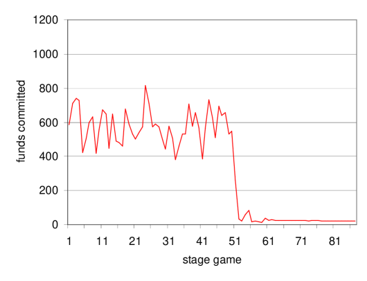
Figure 2: Total liquidity - low delay costs

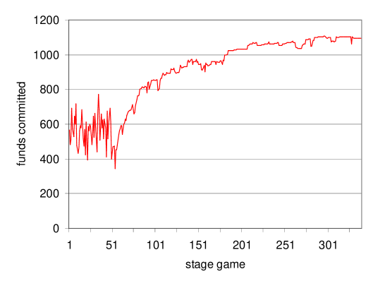
Figure 3: Total liquidity - high delay costs

We find that convergence always occurs - on an aggregate level within a narrow range. A priori, learning might be sensitive to initial observations, and hence it might be subjected to drastic differences in the final ”conclusions”. The consistency of the learning process is illustrated in Figure 4, where we plot the converged-to value of $\sum a_{i}$ (i.e. the total liquidity committed) across plays, for different parameter specifications. Due to randomness - which makes histories necessarily different - the ”learned” liquidity level $\sum a_{i}$ clearly differ, but they do so within small ranges.

It should be noted that while the system consistently ”learns” the same level of total liquidity, this can represent many configurations of single banks’ liquidity choices. Hence, our simulation don’t show that always the same equilibrium is reached; rather, that the equilibria that are reached are characterized by a narrow span of total liquidity in the system. Given the symmetry of the model, it is clear that for any equilibrium (i.e. any equilibrium profile of actions $\left(a_{1},a_{2}...a_{N}\right)$), there are many other equilibria obtained via a permutation of the actions between the players that yield to same total liquidity on the system level.

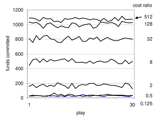
Figure 4: Total equilibrium liquidity across plays

Another interesting feature of the model is its ability to match a well known empirical fact: a low ratio of available liquidity to daily payments (”netting ratio”), which in turn implies high levels of liquidity recycling. Because the system processes on average $10.000$ payments a day, the above results imply that the ratio in our simulation is between $0.5\%$ and $10.4\%$. For comparison, CHAPS Sterling’s netting ratio is $15\%$ (James 2004) and in Fedwire as low as $2.2\%$. The real netting ratios are bound to be higher due to the fact that payments in them are of varying sizes in contrast to the more fluid unit size payments modelled here.

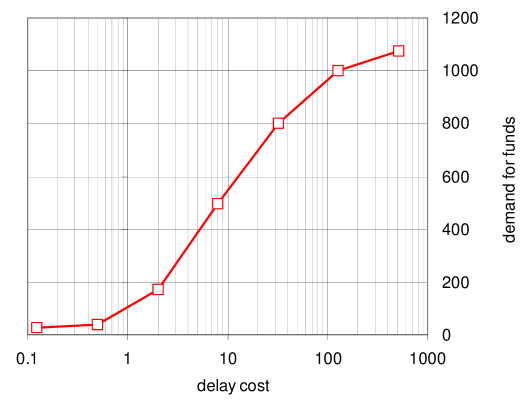
Figure 5: Liquidity as a function of delay costs

Figure 5 shows the equilibrium demand for intraday credit as a function of the cost ratio. This function is S-shaped in the exponential delay cost scale, that is, it is relatively flat at both low and high levels of delay costs. At comparatively low delay costs banks evidently commit little liquidity; hence the return for increasing liquidity holdings are high, and so a little more liquidity suffices to cope with increased delay costs. As a consequence, for low delay cost levels the demand curve is flat. Consider now the situation with high delay costs. There, the liquidity committed is high and returns to increasing liquidity are low, so one might think that an increase in delay costs calls for high extra amounts of liquidity. However, this is not the case, because gains from liquidity indeed diminish above a certain level when all payments can be made promptly. Hence, for high delay costs, liquidity demand is insensitive to further increases in delay costs, and the demand curve is flat again. In between these two extremes, the demand for liquidity increases exponentially with delay costs.

We find that delays in the system increase exponentially as banks reduce the amount of liquidity when this is relatively expensive compared to delaying payments. The phenomenon is known as ”deadweight losses” (Angelini 1998) or ”gridlocks” (Bech and Soramäki 2002) in payment systems. Figure 6 shows the relationship between system liquidity and payment delays. In intuitive terms, the reason of this exponential pattern is the following. First, a bank that reduces its liquidity holdings might have to delay its outgoing payments. Second, as a consequence, the receivers of the delayed payments may in turn need to delay their own payments, causing further downstream delays and so on. Hence, a decrease of a unit of liquidity may cause multiple units to be delays. Third, such a chain of delays - and hence this multiplicative effect - is more likely and longer, the lower the liquidity possessed by the banks. Thus the total effect of liquidity reduction acts in a compounded (exponential) fashion.

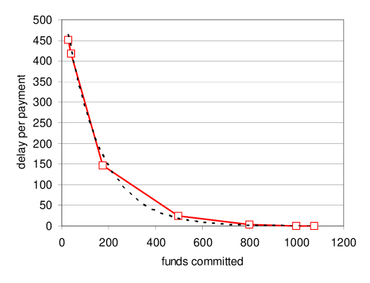
Figure 6: Delays as a function of liquidity

An interesting question is how good the performance of the banks is in absolute terms. To understand this we compare the payoffs received by the banks through adaptation with two extreme strategies:

a) all banks delay all payments to the end of the day;

b) all banks commit enough liquidity to be able to process all payments promptly.

The comparison between the performance of these two pure strategies and the learned strategy is shown in Figure 7. For any cost ratio, the adaptive banks obtain better payoffs than any of the two extreme strategies - except for the case with high liquidity costs when the costs are equal. Banks manage to learn a convenient trade-off between delay and liquidity costs. On the contrary, the strategy under a) becomes quickly very expensive as delay costs increase, and the strategy under b) is exceedingly expensive when delays are not costly.

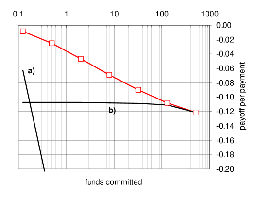
Figure 7: Comparison of strategies: a) min liquidity; b) min delays

3.3 Impact of network size

In order to investigate the impact of system size on the results presented in the previous section, we ran simulations varying the number of participants. To ensure comparability, we kept the number of payments constant across simulations and maintained the network complete.

We observe that liquidity demand increases with the system size, and the increase is more pronounced the higher the delay costs. For example, the demand function is unchanged at low delay cost while, for high delay costs, a 50-bank system requires $215\%$ the liquidity needed in a 15-bank system.

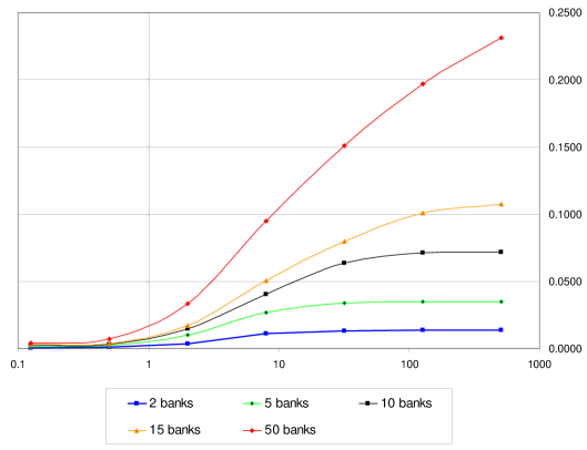
Figure 8: The effect of system size on the demand for liquidity

Similar results hold about delays. The relationship between liquidity committed and delays remains close to exponential irrespective of system size; however, larger systems experience more delays, for any level of initial liquidity (see Figure 9).

An intuitive explanation of these phenomena could be the following. First, note that if the number of participants is increased by a factor $x$ (keeping turnover constant), the volatility of the balance of each bank is multiplied by a factor $1/x^{\prime}>1/x$ - we show this in a moment. Second, suppose that i) the optimal $a_{i}$ is proportional to the volatility of a bank’s balance $\delta$ (i.e. $a_{i}=z\delta$) and that ii) banks post all the same amount of liquidity (i.e. $a_{i}=a_{j}$). It then simply follows that the total amount of liquidity increases with the system’s size: $\left(nx\right)z\frac{\delta}{x^{\prime}}>nz\delta$ (here $nx$ is the number of banks in the larger system, and $\frac{\delta}{x^{\prime}}$ the corresponding volatility of balances).

The key point is that, if the number of participants is increased (keeping turnover constant), the volatility of banks balances rises more than proportionally. To see why this is the case, consider the simplified but illustrative situation where liquidity is abundant, so there are no delays. In this case, a bank’s net position is the sum of a series of random perturbations (incoming and outgoing payments), equally likely to affect it positively and negatively. In other words, a bank’s net position is a random walk, whose value after $n$ perturbations averages zero, with a standard deviation $\sqrt{n}$. By increasing the system size by a factor $x$, the orders are distributed over more banks, so the average number of perturbations for any given time interval is multiplied by $1/x<1$. Accordingly, the standard deviation of the balances at the end of any time interval is multiplied by $1/x^{\prime}=\sqrt{1/x}>1/x$.

3.4 Throughput guidelines

Some interbank payment systems have guidelines on payment submission jointly agreed upon by the system participants. The rationale for throughput guidelines is to induce early settlement in order to e.g. reduce operational risk or perceived coordination failures among participant. For example, if a large chunk of payments are settled late in the day, an operational incident would be more severe as more payments could potentially remain unsettled before close of the payment system and the financial markets where banks balance their end-of-day liquidity positions.

We simulate a particular realization of throughput guidelines by introducing an additional penalty charge for delays that last longer than one tenth of the settlement day (i.e. 1000 time units). The penalty charge is set to 64, in order to sufficiently penalize non-compliance with the rules.

Figure 10 shows the impact of the throughput guidelines on the amount of liquidity committed by the banks. When delay costs are high, banks already commit enough liquidity to avoid long delays, so the throughput guidelines have no effect. They do however, in the case of low delays costs, induce banks to commit more liquidity. Not surprisingly, this comes at a cost to the banks, which are forced away from their first-best choice. The increase in costs are of the order of 70% at the lowest level of delay costs, and 20% at the second lowest. The payoff comparison is shown in Figure 11.

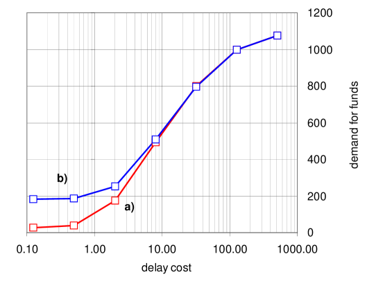
Figure 9: Impact of throughput guidelines (b) on liquidity

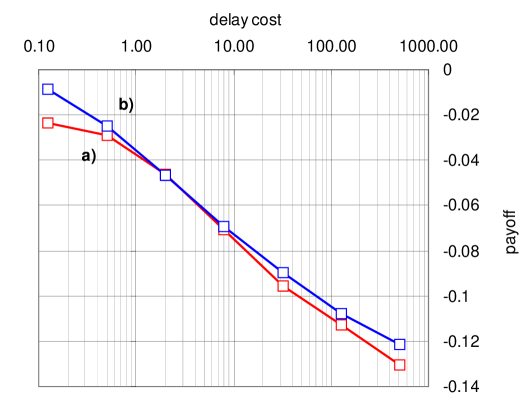
Figure 10: Impact of throughput guidelines (b) on payoffs

3.5 Operational incident

Short term outages by banks in the payment system are rare in actual payment systems, but do take place occasionally. In a typical scenario a participating bank experiences problems connecting to the system due to temporal unavailability of IT systems or telecommunication facilities. Due to the design of the payment systems, a disconnected bank can in such situations generally still receive payments to its account at the central bank, but cannot submit instructions to pay from its account. Unless other banks stop paying to the troubled bank, it quickly becomes a liquidity sink, and the liquidity available for settling payments at other banks is reduced.

In this set of simulations we ask the question of how much liquidity banks would wish to commit in such a situation, i.e. what is the impact of an operational outage on the demand for intraday credit. The banks are assumed to be unaware of the possible incident, and unable to discriminate among their counterparts, so the intraday liquidity management rule under Eq. 4 is still adopted. Under these assumptions, we simulated a scenario where a randomly selected bank can receive, but cannot send payments for the first half of the settlement day. On average, this means that up to $T/2N=10.000/(2\cdot 15)\simeq 333$ liquidity units cannot be used by other banks as a source of liquidity. Depending on the delay cost, this figure varies between 1900% and 30% of the average total liquidity injected in the system at the beginning of the day (the first figure being for the case when both delay cost and liquidity demand are low, and the second for when costs liquidity demand are both high).

We found that the effect of operational incidents on the demand for liquidity is highest at a relative delay/liquidity cost ratio of $2$ - hence fairly low in the range; at this point, the increase in intraday credit demand is $144$ units, or an increase of $85\%$. It should be noted that banks do not compensate for the full amount of liquidity ”trapped” by the distressed bank, but prefer to partly make up for that, and partly increase delays. For higher delay costs, delays remain approximately unchanged compared to the scenario without the incident. Finally, when delay costs are lower than liquidity costs (i.e. for a cost ratio $<$1), banks prefer to hold about the same amount of liquidity as without the incident, and experience the delays caused by the reduced liquidity. In this case, the impact of an operational incident increases both the demand for liquidity (but less than what was trapped) and delays - more so the one which is less costly.

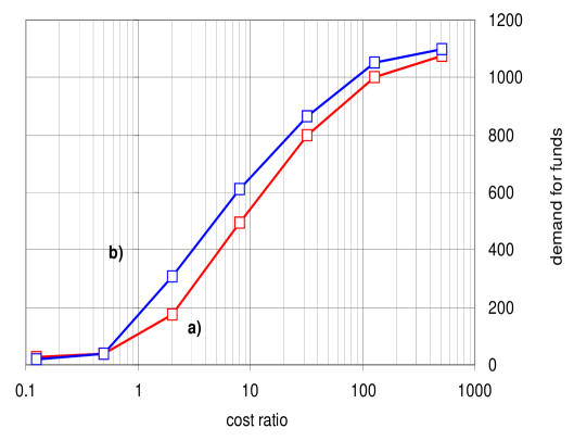
Figure 11: Liquidity - normal circumstances (a) and operational incidents (b)

Figure 12: Delays as a function of cost ratio (b: incident)

4 Summary and conclusions

In this paper we developed an agent-based, adaptive model of banks in a payment system. Our main focus is on the demand for intraday credit under alternative scenarios: i) a ”benchmark” scenario, where payments flows are determined by the initial liquidity, and by an exogenous arrival of payment instructions; ii) a system where, in addition, throughput guidelines are exogenously imposed iii) a system subject to operational incidents.

It is well known that the demand for intraday credit is generated by a trade-off between the costs associated with delaying payments, and liquidity costs. Simulating the model for different parameter values, we were able to draw with some precision a liquidity demand function, which turns out to be is an S-shaped function of the delay / liquidity cost ratio. We also looked at the costs experienced by the banks, as a function of the model’s parameters. By the process of individual payoff maximization, banks adjust their demand for liquidity up (reducing delays) when delay costs increase, and down (increasing delays), when they rise. Interestingly however, the absolute delay cost remains approximately constant when the ratio delay/liquidity costs changes. As expected, the demand for intraday credit is increased by an operational incident. However, this effect is found to be important only if liquidity is costly compared to delaying payments. Likewise, throughput guidelines increase the demand for intraday credit - as banks try to avoid penalties for not adhering to them. In total this reduces the payoffs of the banks. Nevertheless, throughput guidelines may be beneficial when additional benefits that are not in the current model are taken into account (among these, benefits related to reducing operational risk).

This model produces realistic behaviour, suggesting that it may be used to investigate a wide array of issues in future applications. A number of extensions are possible. First, alternative specifications for the instruction arrival process may be applied (see e.g. Beyeler at al. (2006)). Alternatively, one could change the assumptions on the banks’ network: while the complete network assumption implicitly adopted here fits well with e.g. the UK CHAPS system, an interesting question is how other topologies such as a scale free network topology such as in Fedwire (Soramäki et al.. 2007) would affect the results. Also, different individual preferences could be investigated. We assumed that banks are risk neutral and interested in maximising their immediate payoffs; it would be interesting to verify if the introduction of risk aversion and / or preferences over expected stream of payoffs may change the results. Finally, more complex behaviour can be easily studied within our model; for example, the ”pay-as-much-as-you-can” rule for queuing payments could be replaced by sender limits. Similarly, more sophisticated strategies can be easily modelled, supposing e.g. that banks keep constant their actions for a number of periods (to gather more data and explore the environment), instead of exploiting after a fixed amount of time what seems to be the best action.

References

- [1] Angelini, P (1998), ‘’An Analysis of Competitive Externalities in Gross Settlement Systems”, Journal of Banking and Finance n. 22, pages 1-18.
- [2] Bank for International Settlements (2006), Statistics on payment and settlement systems in selected countries - Figures for 2005 - Preliminary version. CPSS Publication No. 75.
- [3] Barto, A G and Sutton, R S (1998), Reinforcement Learning: an introduction. MIT Press, Cambridge, Massachusetts.
- [4] Barto, A G, Sutton, R S and Brouwer, P S (1981), ”Associative search network: A reinforcement learning associative memory”. Biological Cybernetics, 40, pages 201-211.
- [5] Bech, M L and Soramäki, K (2002), ”Liquidity, gridlocks and bank failures in large value payment systems”. in E-money and payment systems Review, Central Banking Publications. London.
- [6] Bech, M L and Garratt, R (2003), ”The intraday liquidity management game”, Journal of Economic Theory, vol. 109(2), pages 198-219.
- [7] Bech, M L and Garratt, R (2006), ”Illiquidity in the Interbank Payment System Following Wide-Scale Disruptions”. Federal Rererve Bank of New York Staff Report No. 239.
- [8] Beyeler, W, Bech, M, Glass, R. and Soramäki K (2006), ”Congestion and Cascades in Payment Systems”. Federal Reserve Bank of New York Staff Report No. 259.
- [9] Blume, L (1993), ”The statistical mechanics of best-response strategy revision”. Games and Economic Behavior, 11, pages 111–145.
- [10] Brown, G W (1951), ”Iterative Solutions of Games by Fictitious Play” in Koopmans T C (Ed.), Activity Analysis of Production and Allocation, New York: Wiley.
- [11] Buckle, S and Campbell, E (2003), ”Settlement bank behaviour in real-time gross settlement payment system”. Bank of England Working paper No. 22.
- [12] Devriese, J and Mitchell J (2006), ”Liquidity Risk in Securities Settlement”, Journal of Banking and Finance, v. 30, iss. 6, pages 1807-1834.
- [13] Ellison, G (1993), ”Learning, local interaction, and coordination”, Econometrica, 61, pages 1047-1072.
- [14] Foster, D P and Young H P (1998), ”On the Nonconvergence of Fictitious Play in Coordination Games”, Games and Economic Behavior, v. 25, iss. 1, pages 79-96.
- [15] Fudenberg, D and Levine D K (1998), ”The Theory of Learning in Games”. MIT Press., Cambridge, Massachusetts.
- [16] James, K and Willison M. (2004), ”Collateral Posting Decisions in CHAPS Sterling”, Bank of England Financial Stability Report, December 2006.
- [17] Kandori. M, Mailath, G J and Rob, R (1993), ”Learning, Mutation, and Long Run Equilibria in Games”, Econometrica, Vol. 61, No. 1. pages 29-56.
- [18] Krishna, V and Sjostrom, T (1995), ”On the Convergence of Fictitious Play”, Mathematics of Operations Research 23(2), pages 479 - 511.
- [19] Lacker, J M (2004), “Payment system disruptions and the federal reserve following September 11, 2001.” Journal of Monetary Economics, Vol. 51, No. 5, pages 935-965.
- [20] McAndrews, J and Potter S M (2002), “The Liquidity Effects of the Events of September 11, 2001”, FRBNY Economic Policy Review, Vol. 8, No. 2, pages 59-79.
- [21] Soramäki, K, Bech, M L, Arnold, J, Glass R J and Beyeler, W E (2006), ”The Topology of Interbank Payment Flows”. Physica A Vol. 379, pages 317-333.
- [22] Schlag, K (1995), ”Why Imitate, and if so, How? A Boundedly Rational Approach to Multi-Armed Bandits”, Journal of Economic Theory 78(1), pages 130–156.
- [23] Watkins, C and Dayan P (1992), ”Technical note: Q-learning”, Machine Learning, 8(3/4), pages 279-292.
- [24] Willison, M (2005), ”Real-Time Gross Settlement and hybrid payments systems: a comparison”, Bank of England Working Paper No. 252.
- [25] Young P (1993), ”The evolution of conventions”, Econometrica 61, pages 57-84.