In search of dying radio sources in the local universe
Abstract
Aims. Up till now very few dying sources were known, presumably because the dying phase is short at centimeter wavelengths. We therefore have tried to improve the statistics on sources that have ceased to be active, or are intermittently active. The latter sources would partly consist of a fossil radio plasma left over from an earlier phase of activity, plus a recently restarted core and radio jets. Improving the statistics of dying sources will give us a better handle on the evolution of radio sources, in particular the frequency and time scales of radio activity.
Methods. We have used the WENSS and NVSS surveys, in order to find sources with steep spectral indices, associated with nearby elliptical galaxies. In the cross correlation we presently used only unresolved sources, with flux densities at 1.4 GHz larger than 10 mJy. The eleven candidates thus obtained were observed with the VLA in various configurations, in order to confirm the steepness of the spectra, and to check whether active structures like flat-spectrum cores and jets are present, perhaps at low levels. We estimated the duration of the active and relic phases by modelling the integrated radio spectra using the standard models of spectral evolution.
Results. We have found six dying sources and three restarted sources, while the remaining two candidates remain unresolved also with the new VLA data and may be Compact Steep Spectrum sources, with an unusually steep spectrum. The typical age of the active phase, as derived by spectral fits, is in the range years. For our sample of dying sources, the age of the relic phase is on average shorter by an order of magnitude than the active phase.
Key Words.:
Radio continuum: galaxies – Galaxies: active1 Introduction
Radio sources associated with elliptical galaxies are supplied with energy from active galactic nuclei via plasma jets or beams (Scheuer Scheuer74 (1974); Begelman et al. Beg84 (1984); Bridle & Perley Bridle84 (1984)). In the active stage the total spectra of the radio sources are usually well approximated by a power law over a wide range of frequencies; spectral breaks at high frequencies, with moderate steepening of the spectrum, are also often observed. The break frequency is related to the age of the source.
After this phase, which may last several years, the activity in the nuclei stops or falls to such a low level that the plasma outflow can no longer be sustained. The radio core, well-defined jets and compact hot-spots will disappear, because these structures are produced by continuous activity. However, the radio lobes may still remain detectable for a long time if they are subject only to radiative losses.
The switch-off of the injection of energetic electrons leads to a second high frequency break with an exponential steepening of the total spectrum of the radio source (Komissarov & Gubanov Kom94 (1994)). This second high frequency break is related to the time passed since the switch-off of the central engine. Therefore “dying” radio galaxies should have steeper high frequency spectra than normal (active) radio galaxies. Current models of radio source physics, based on the assumption that radiative losses are dominant, predict the existence of a large population of radio sources that are bright at 100 MHz, but have a steep spectrum around 1 GHz. However, such sources are not commonly found.
According to Giovannini et al. (Giov88 (1988)) only few percent of objects in a sample of B2 and 3C radio galaxies have the characteristics of a dying radio galaxy. The first unambiguous example of such a source was given by Cordey (Cordey87 (1987)); see also more recent data on this source in Jamrozy et al. (Jamrozy04 (2004)). Up till now only four other sources have been discovered (e.g. Venturi et al. Venturi98 (1998); Murgia et al. Murgia05 (2005)).
In the literature some possible dying sources, located in rich clusters, are mentioned, but these can be interpreted either as remnants of dying radio galaxies at the point of being disrupted by a particularly turbulent environment (Slee et al. Slee01 (2001)), or as old radio lobes that are compressed by shock waves (Enßlin & Gopal-Krishna Ens01 (2001)). However the identification of former host galaxies is problematic and thus their association with dying radio sources is uncertain.
It is also possible that radio galaxies may be active intermittently; in that case one may find fossil radio plasma left over from an earlier phase of activity, while newly restarted core and radio jets are visible as well. Examples of restarting activity in the presence of fossil radio lobes are 3C 338 and 3C 317 (Roettiger et al. Roet93 (1993); Venturi et al. Venturi04 (2004)); intermittent jet activity in 4C29.30 is discussed by Jamrozy et al. (Jamrozy07 (2007)). Restarting activity has now also been found in Compact Steep Spectrum (CSS) sources (Marecki et al. Marecki06 (2006)).
The ”double-double radio sources” form an interesting class of restarting activity, in which new radio lobes can be seen close to the nucleus, while an older pair of lobes is still present farther out (Schoenmaker et al. Schoenmaker00 (2000)). At present about a dozen of such sources are known (see Jamrozy et al. Jamrozy07 (2007) and references therein).
Dying radio sources and intermittent radio galaxies are more easily detectable at low frequencies: a search for this type of object should be performed using surveys at frequencies below 1 GHz.
In this paper we describe a search for dying sources and discuss the properties of the sources we have found so far.
In Sect. 2 we briefly describe the selection of the sample and the radio and optical observations. In Sect. 3 we show radio contour maps and integrated spectra of the sources in the sample. In Sect. 4 we give some comments on individual sources and in Sect. 5 we discuss the properties of the dying sources. Finally in Sect. 6 we summarize the results obtained in this paper.
All intrinsic parameters (radio power, absolute magnitudes, sizes) were calculated with km s-1 Mpc-1, , . Spectral indices are defined according to .
2 Selection of the sample and observations
2.1 The sample
Since dying radio galaxies and intermittent radio sources are more easily detected at low frequencies, the Westerbork Northern Sky Survey (WENSS; Rengelink et al. Renge97 (1997)) at 325 MHz is particularly well-suited for this purpose. As a starting point we have used the work done by De Breuck et al. (debreuck00 (2000)); while their aim was to find high-redshift radio galaxies, we are instead interested in steep spectrum radio sources identified with bright galaxies: these are our prime dying source candidates. De Breuck et al. (debreuck00 (2000)) correlated the WENSS and NVSS (Condon et al. Condon98 (1998)) catalogues using a search radius of 10 arcsec centred on the WENSS positions. They obtained spectral indices for 143000 sources with mJy. Only unresolved sources (angular cutoff arcmin) were considered. A further condition was mJy. We note that especially this last criterion may lead to the loss of many steep spectrum sources, because De Breuck et al. (debreuck00 (2000)) effectively used only that part of WENSS with flux densities above mJy. Thus they obtained a sample of 343 sources with spectral indices . We plan to extend in the near future the search for dying radio sources also to 1400 MHz flux densities below 10 mJy. Optical identifications were done using the digitized POSS-I and were listed in their table A.4. We checked all the identifications listed and estimated galaxy magnitudes following the procedure described in de Ruiter et al. (deruiter98 (1998)). Selecting from list A.4 only sources associated with an elliptical galaxy with we obtained 11 candidate dying sources.


2.2 Radio observations
In order to determine whether the integrated radio spectra of these dying source candidates are really steep also at high frequencies we have observed the sample in snap-shot mode with the VLA D-array at 4.8 and 8.4 GHz. The sources are sufficiently compact ( arcmin) for being only slightly resolved at high frequency and therefore we are able to measure the total flux density. However, we need to know whether active radio structures such as radio cores, jets and hot spots, are present. In order to fill this gap in our knowledge we also performed VLA B-array observations, at 1.4, 4.8 and 8.4 GHz.
Four of the most promising objects were observed with the VLA A-array at 327 MHz. In this way we have obtained spectral information (between 1.4 GHz and 327 MHz) on the source components.
A summary of the observations, including the array, frequency, length of observation, beam size and r.m.s. noise is given in Table 1. A bandwidth of 50 MHz was used for the B- and D-array, while the observations with the A-array were done in line mode.
Calibration and imaging was done using the NRAO Astronomical Image Processing System (AIPS) in the standard way.
2.3 Optical observations
Optical spectroscopy was done with the DOLORES spectrograph installed at the Nasmyth B focus of the 3.5-m Galileo telescope on the Roque de los Muchachos in La Palma, Spain. The observations were performed in service mode during several nights between Jan 29 2004 and Aug 5 2005. We used the LR-B grism and a slit size between 1.0 and 1.5 arcsec, depending on the seeing conditions during the observations. The dispersion was 2.8 Å per pixel and the spectral resolution about 11 Å. The typical useful spectral range is to Å with increasing fringing beyond 7200 Å. The slit orientation was adjusted to maximise the number of spectra obtained with a single setup.

The reduction of the spectra was carried out using the LONGSLIT package of NOAO’s IRAF reduction software. A bias frame was constructed by averaging ‘zero second’ exposures taken at the end of the night. This was subtracted from every non-bias frame. The pixel-to-pixel variations were calibrated using internal flats. The sky contribution was removed by subtracting a sky spectrum obtained by fitting a polynomial to the intensities measured along the spatial direction excluding the vicinity of objects. One-dimensional spectra were extracted by averaging in the spatial direction over an aperture as large as the spatial extent of the source. Wavelength calibration was carried out by measuring the positions on the frames of known emission lines from a He-lamp and a flux calibration was obtained from a comparison with spectra of spectro-photometric standard stars.
As the main goal of our spectroscopic observations was the determination of the redshifts, the exposure times were kept as short as possible. Almost all spectra show the 4000 Å break, the Ca H and K lines, as well as the MgI and NaI absorption lines. Most sources show no obvious emission lines, except WNB1408.8+463014, which may have H in emission; however that part of the spectrum is strongly affected by fringing. The resulting redshifts are compiled in Table 2. In addition we report the redshifts of some of the ambient objects which were covered by the slit (see Table 3).
3 Results
3.1 Radio maps and integrated spectra
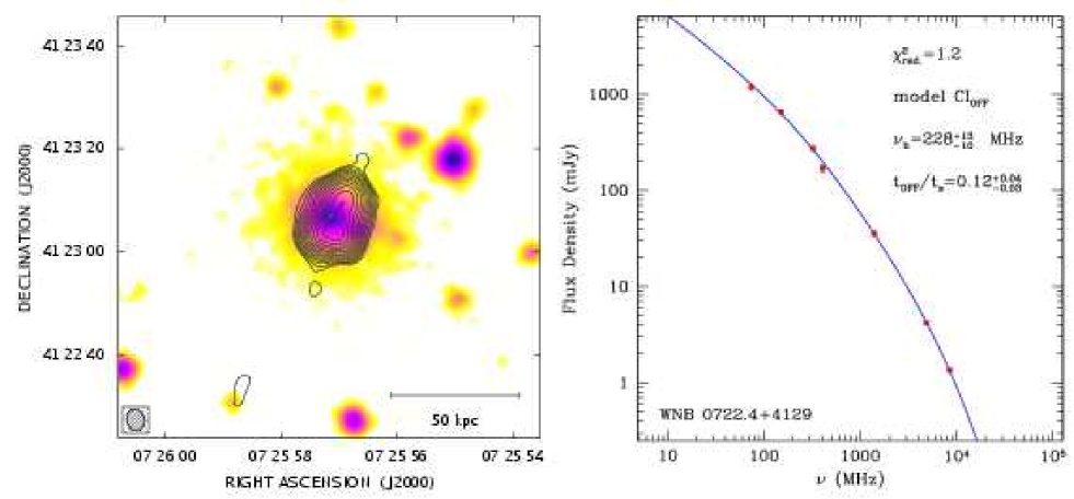
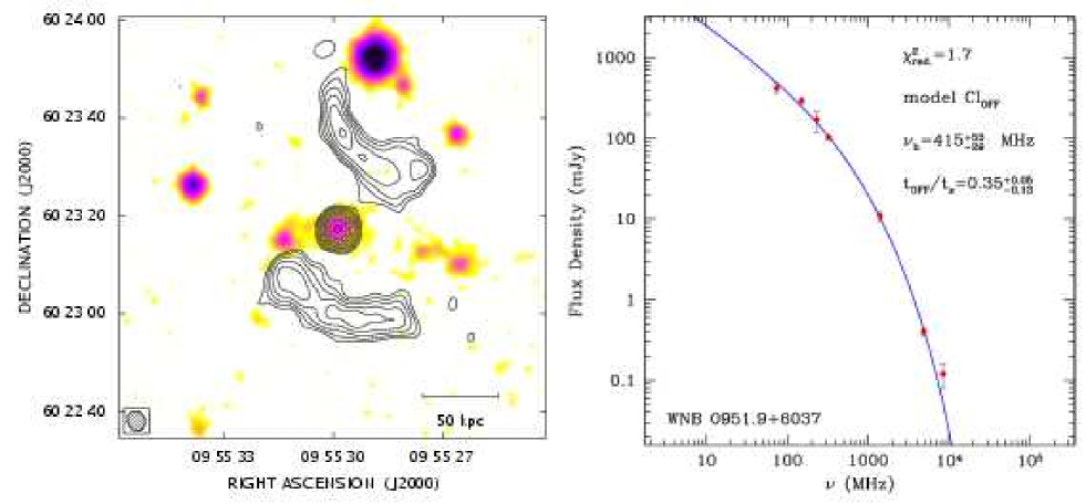
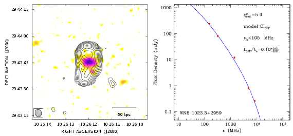
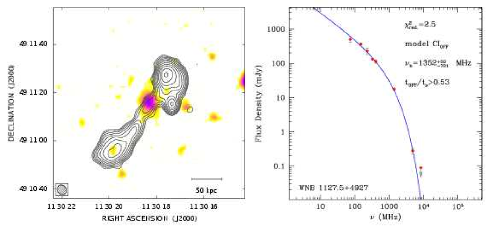
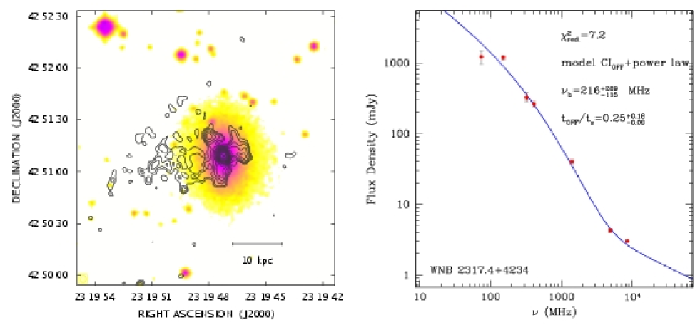
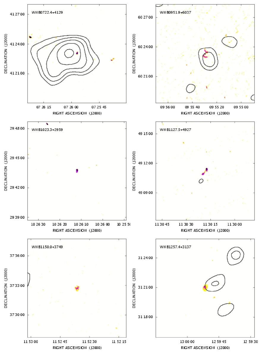
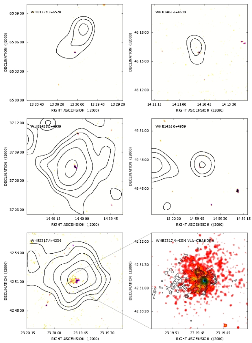
Images of the sources are given in Figs. 1 to 11. The contours of the B-array observations at 1.4 GHz are superposed on DSS2 red images. Contour maps of the A-array observations at 327 MHz, shown in Figs. 12 to 15 are superposed on grey scale images of the spectral index (between 327 MHz and 1.4 GHz). D-array images are not shown, since all sources are unresolved.
Measured source, and if possible also component, parameters are given in Table 2. We give the position of the associated optical galaxy and of the source radio core when present. We also give the total flux of the source or that of the components together with the corresponding observing frequency. Usually only the central component is detected at high frequency. The size of the source corresponds to the full-width-half-maximum (FWHM) of a Gaussian fit or to the largest angular size (LAS), using the lowest reliable contour.
A dying source should show exponential steepening of its total spectrum. The sources of our sample were selected on the basis of their spectral steepness between 1.4 GHz and 325 MHz, but we also collected other spectral information: in addition to the D-array observations done at 5 and 8.4 GHz, we also made use of CATS (the on-line Astrophysical CATalogs support System, at http://cats.sao.ru/), thus recovering data at different frequencies. The 74 MHz flux densities were determined directly from NRAO VLSS images that are available on-line (at URL: http://lwa.nrl.navy.mil/VLSS/). The results of this search are shown in Table 4, where all the available data for each individual source are listed.
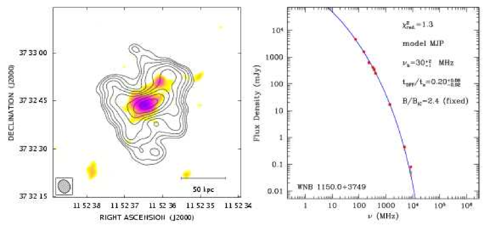
The total spectra of most of the radio sources in our sample show a quasi-exponential cutoff in the frequency range between 74 MHz and 8.4 GHz. For some sources the spectral cutoff is particularly strong (WNB0951.9+6037, WNB1127.5+4927, and WNB1150.0+3749). In some others (WNB1328.3+6520 and WNB1458.0+4959) the curvature is less pronounced and the integrated spectrum is almost a power law in the considered frequency range. Finally, WNB1408.8+4630, WNB1438.0+3720 and WNB2317.4+4234 show evident flattening of the integrated spectrum at high frequency. This flattening is due to the presence of a core-jet component that dominates the spectrum at the highest frequencies. This is confirmed by the images at higher resolution (not shown), in which only the core is visible.
3.2 Spectral indices of source components
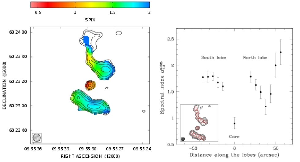
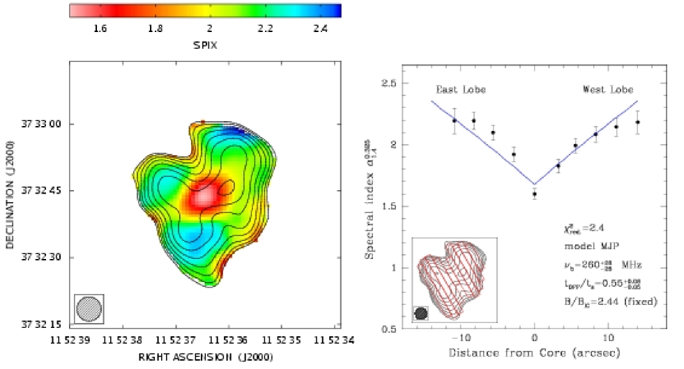
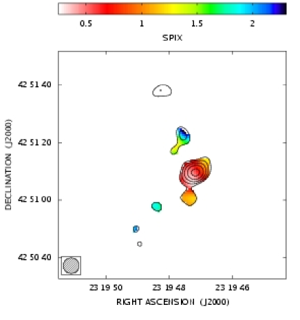
WNB0951.9+6037, WNB1127.5+4927, WNB1150.0+3749, and WNB2317.4+4234 were also observed at 327 MHz with the VLA A-array. Spectral index maps, using both 327 MHz and 1.4 GHz data at 6 arcsec resolution, are shown in the left-hand panels of Figs. 12 to 15. In the right-hand panels the spectral index distributions are shown, as computed in boxes along the ridge line, or all over the source, in the way shown in the inset.
In WNB0951.9+6037 the northern lobe (or tail) has in the centre, and steepens going outwards in both directions to values of and at the respective ends. The south lobe has a uniform spectral index of . Note that also the central component of this source has a steep spectrum, with . In WNB1127.5+4927 the spectral indices of the two lobes are almost constant with values of the order of 1.3. At most there might be a very slight steepening of no more than (see Fig. 13). In WNB1150.0+3749 the spectral index varies from in the source centre to in the outer parts. In WNB2317.4+4234 only the head of the tail is visible at 327 MHz; it has .
4 Comments on individual sources
-
•
WNB0722.4+4129: a small asymmetric double without a core. It is completely resolved out in the B-array observations at 5 and 8.4 GHz.
-
•
WNB0951.9+6037: the central component is detected in the B-array observation at 8.4 GHz but not at 4.8 GHz due to the higher rms noise on the 4.8 GHz map. Since it has and it is difficult to consider this an active core. At 327 MHz and 1.4 GHz the source structure is very similar, the northern component being slightly more elongated at 327 MHz.
-
•
WNB1023.3+2959: a small asymmetric double without core. It is completely resolved out in the B-array observations at 5 and 8.4 GHz.
-
•
WNB1127.5+4927: a classical double source with a compact (apparently background) source superimposed on the western lobe. No core has been detected. At 5 and 8.4 GHz (B-array) only the background source is detected. The double source structure is very similar at 327 MHz and 1.4 GHz, but the background source is not detected at 327 MHz due to its flat spectral index ().
-
•
WNB1150.0+3749: a source with amorphous structure. It may be a small double source without a core and is completely resolved out in the B-array observations at 5 and 8.4 GHz. At 327 MHz the radio structure is very similar to the one at 1.4 GHz.
-
•
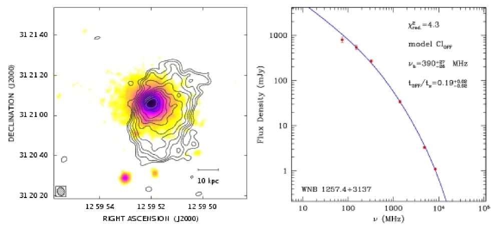
WNB1257.4+3137: a source with amorphous structure at 1.4 GHz. At 4.8 GHz only the central component is still visible, which, however, is completely resolved out at 8.4 GHz.
-
•
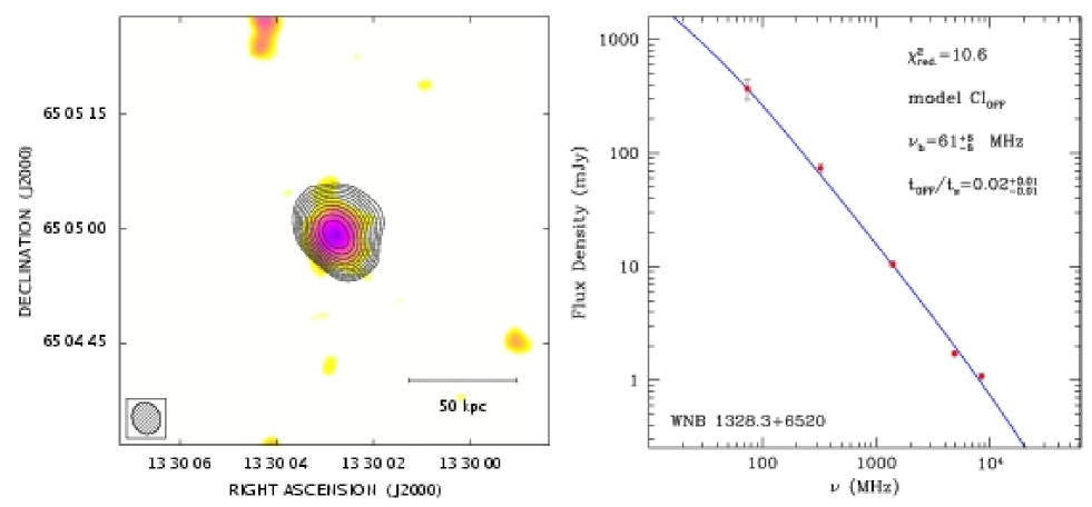
WNB1328.3+6520: a compact radio source with a very steep spectrum. It is detected in all B-array observations. This source resembles a Compact Steep Spectrum (CSS) source, but with an unusually steep spectrum.
-
•
WNB1408.8+4630: apparently this source has one-sided morphology. The galaxy position coincides with the bright compact component. Much fainter emission extends to the south-west. Perhaps this is a core-jet radio source or, alternatively, a small head-tail source. The bright component has and is probably the radio core. The very steep spectrum low frequency emission probably comes from an extended component that is not seen at frequencies GHz. However, the integrated spectrum shows flattening at high frequencies due to the presence of the flat-spectrum core.
-
•
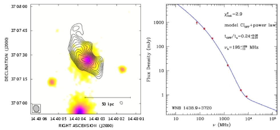
WNB1438.0+372: a small bent radio source at 1.4 GHz. A core () is detected at higher frequencies. This radio source may be a small wide angle tail (WAT).
-
•
WNB1458.0+4959: a very compact radio source at 1.4 and 5.0 GHz. It is not detected at 8.4 GHz. This source resembles a CSS source, but with an unusually steep spectrum.
-
•
WNB2317.4+4234: a head-tail source. The tail is very weak and only the head is detected at 5 and 8.4 GHz. At 327 MHz the tail cannot be seen because the rms noise of the map is rather high. The head has and . The associated galaxy is NGC 7618.
5 Discussion
5.1 Morphological properties and radio cores
¿From a morphological point of view the sources discussed here form a rather mixed bag. The only common characteristic is their small angular size, but of course this is due to the selection bias ( arcmin). Since the sources cover a relatively large redshift range (from 0.02 up to about 0.26) the linear sizes show more variety, although in a power-linear size plot these sources mix with, for example, the general sample of B2 radio galaxies. It should be noted however, that the morphologies found in this sample are very different from those of the B2 radio galaxies, but, again, this may be due to the size selection imposed on the sample of candidate dying sources.
A flat spectrum radio core is unambiguously present only in a minority of cases: using the higher frequency data we detected a radio core in three sources, while we can put upper limits on the core luminosity for the other ones. Radio cores might still be present at lower levels without flattening the spectrum significantly. We find that nine sources have a ratio (of which one is a detection at the level of ), while only two are above this (of order ). ¿From the relation between core and total luminosity given by Giovannini et al. (Giov88 (1988)) we would have expected a ratio for about half of the sources. Therefore, even allowing for the selection bias introduced by the steepness of the spectra, the cores in the present sample are quite weak and this fact strengthens the suspicion that the majority in our sample may be genuine dying radio sources.
5.2 Equipartition parameters
We assume that the radio sources contain relativistic particles and magnetic fields uniformly distributed and in energy equipartition conditions. The equipartition parameters (total energy , energy density and magnetic field ) are generally computed assuming that the relativistic particle energies are confined between a minimum and a maximum , corresponding to the observable radio frequency range, typically 10 MHz - 100 GHz (see, e.g., Pacholczyk Pach70 (1970)). This choice minimizes the source energetics required by the observed radiation in the radio band. However, a fixed frequency range corresponds to an energy range that depends on the source magnetic field, which may change from source to source. Furthermore, as pointed out by Brunetti et al. (Brunetti97 (1997)) a fixed frequency range computation would miss the contribution from lower energy electrons, since the corresponding to 10 MHz is larger than 200 MeV for ; this missing contribution can be very large. Because of this we have computed, wherever possible, the equipartition parameters assuming a fixed low energy cutoff = 10 MeV (for this choice see Brunetti et al. Brunetti97 (1997)). Intrinsic parameters, including equipartition parameters, are listed in Table 5.
For a power law energy distribution () the equipartition magnetic field is given by the following expression
| (1) |
where is the spectral index (assumed to be 0.8), the source volume in kpc3, a reference frequency in GHz, the monochromatic luminosity at in W/Hz, the ratio of proton to electron energy (assumed to be one) and a quantity in the range for .
As far as the choice of is concerned (see Sect. 5.3 for details about the parameters used) we note that beyond no electrons are present and the energy contribution in the range from to is always much less than that below . Furthermore it turns out that in the equipartition formula can be neglected.
The equipartition parameters computed in this way are reported in Table 5. A comparison with fixed frequency range calculations shows that the values of our are larger by up to a factor two.
5.3 Modelling the integrated radio spectra
The radiative energy losses are assumed to be dominant with respect to other processes (e.g. adiabatic losses). The pitch angles of the radiating electrons are assumed to be continually isotropized in a time that is shorter than the radiative time scale. According to this assumption the synchrotron energy losses are statistically the same for all electrons. After its birth the source is supposed to be fuelled at a constant rate (i.e. the continuous injection phase) by the nuclear activity, for a duration . The injected particles are assumed to have a power law energy spectrum , which will result in a power law radiation spectrum with spectral index . In this phase the source radio spectrum changes as a function of time in a way described by the shift of break frequency to ever lower values as the time, , increases:
| (2) |
where and are the source magnetic field and the inverse Compton equivalent magnetic field, respectively. Below and above the spectral indices are respectively and +0.5.
At the time the power supply from the nucleus is switched-off. After that a new phase of duration begins (i.e. the relic phase). A new break frequency then appears, beyond which the radiation spectrum drops exponentially. This second high frequency break is related to the first by:
| (3) |
where is the total source age (see e.g. Komissarov & Gubanov Kom94 (1994); Slee et al. Slee01 (2001)).
Thus, the above synchrotron model (hereafter CIOFF) is described by four parameters:
-
i)
, the injection spectral index;
-
ii)
, the lowest break frequency;
-
iii)
, the relic to total source age ratio;
-
iv)
, the flux normalization.
In the CIOFF model the magnetic field strength is assumed to be uniform within the source. Slee et al. (Slee01 (2001)) and Murgia (in prep.) propose a more sophisticated model (MJP), which takes into account diffusion of synchrotron electrons in a magnetic field with a Gaussian distribution of field strengths. Compared to the basic CIOFF model the MJP model is characterized by two more free parameters:
-
v)
, the ratio of the rms to the inverse Compton magnetic field;
-
vi)
, the electron diffusion efficiency.
If the rms magnetic field is stronger than the inverse Compton magnetic field () and the electron diffusion is low () the spectrum beyond is less steep than the exponential drop in the CIOFF model. The differences in the shape of the spectral cutoff are significant only for extremely steep spectrum sources, i.e. if MHz and . For this reason we fitted the total spectra of all sources with the CIOFF model, excluding WNB1150.0+3749. In this case only the fit obtained by the MJP model was definitely better. This is not so surprising as WNB1150.0+3749 is the source with the steepest spectrum of all. The model fit is represented by a solid line in the right-hand panels of Figs. 1 to 11, where we also show the reduced and the best fit parameters. The most difficult parameter to constrain is , since its determination requires flux density measurements at frequencies below 74 MHz, our lowest frequency. For this reason, we preferred to keep its value fixed to in the fitting procedure. This value is characteristic of the spectra of jets and hot spots of many active radio galaxies and can be assumed as a plausible injection spectral index. If we used instead, we obtain similar results, although the average is then slightly worse. Beyond the high-frequency spectral cutoff in WNB1150.0+3749 the spectral drop is flatter than exponential. Therefore, this spectrum was fitted with an MJP model in which we fixed the diffusion efficiency at and the ratio at . The value of was derived by adopting for the equipartion magnetic field strength G.
Overall the fits are quite good. The worst cases are WNB1328.3+6520 and WNB1458.0+4959, which happen to be the two most compact sources of our sample. Apart from these two objects, we find that is typically in the range 100 MHz - 1 GHz, while confirming that these really are radio galaxies in which the fuelling of relativistic electrons has been in an off-state by a significant amount of time. The spectra of WNB1328.3+6520 and WNB1458.0+4959 are steep power laws. According to the adopted model we see the aged spectrum of the continuous injection phase. Thus, these sources may not yet be in the dying phase.
In general the radio cores are very weak, most having . The sources WNB1408.8+4630, WNB1438.0+3720 and WNB2317.4+4234 are different cases. Their low frequency spectrum is rather steep, but strongly flattens above 1.4 GHz, due to the presence of a bright core that is clearly detected in the 5 and 8.4 GHz B-array images. These cores have a flat spectrum characterized by between these two frequencies and are likely still active. In order to account for these components in the spectral fit, we added a power law to the CIOFF model, using the observed spectral index and flux density as the normalization. In these three cases we may be observing fading lobes (produced by a previous duty cycle), in conjunction with restarting activity in the core.
5.4 Modelling the spectral index profiles
In three cases (WNB0951.9+6037, WNB1127.5+4927 and WNB1150.0+3749) the profile of the 0.3 to 1.4 GHz spectral index can be traced all along the lobes. The traces are shown in the right-hand panels of Figs. 12 to 14. Assuming a constant source expansion velocity the spectral index at a given distance from the core can be related to the synchrotron age of the electrons at that location. In particular, if the electrons were injected inside the core during the active phase, we expect that the break frequency scales as:
| (4) |
where the distance ranges from at the core, up to at the edge of the source. Thus, the break frequency along the lobes varies from a minimum of , at , up to a maximum of , at . The two limiting break frequencies and are exactly the same as given in Eqs. (2) and (3), respectively.
WNB0951.9+6037 has a Z-shape and this complicates the interpretation of the spectral index profile: it is not possible to identify the regions where the electrons were injected during the active phase. On the other hand, in WNB1127.5+4927 and WNB1150.0+3749 the spectral index steepens going from the regions near the core outward. Thus, it is plausible that the electrons were injected near the core and subsequently flowed outward. We fitted the spectral index trend in WNB1127.5+4927 with the CIOFF model and obtained a minimum break frequency of MHz with . Such values are in very good agreement with those found from the fit of the global spectrum. In WNB1150.0+3749 the fit of the MJP model to the observed spectral index trend gives MHz and . For this source the CIOFF model produces a significantly worse fit of the spectral trend than the MJP model, in good agreement with the fit obtained for the integrated spectrum. We note that a source in which the activity had been stopped already for a long time is expected to have and thus should have a rather constant spectral index distribution. Strong spectral index variations along the lobes can be observed only if , i.e. just after the injection has been switched off.
5.5 Radiative ages
Assuming a constant magnetic field and no expansion after the switch-off, the total source age can be calculated from the break frequency, :
| (5) |
where the synchrotron age is in Myr, the magnetic field in G, the break frequency in GHz, while the inverse Compton equivalent field is G.
By adopting the equipartition value for the magnetic field strength we can thus derive the synchrotron age . Finally, from the ratio , which is also given by the fit, we can determine the absolute durations of the active and relic phases, and . The typical ages of the active phase are in the range yrs. The relic phase is typically shorter by an order of magnitude, but there are cases in which the duration of the relic phase is comparable, if not longer, than that of the active phase (e.g. WNB1127.5+4927 and WNB1150.0+3749). It is quite hard to get a firm estimate on the relative ages of the active and dying phases based purely on source statistics, as we would need unbiased and complete samples, constructed in the same way, of both dying and active sources. However, we do have some general data on the identification of WENSS sources with nearby galaxies (de Ruiter et al., in preparation): preliminary identification work gives us a sample of about 350 radio sources, extracted from the WENSS survey, if we follow the same criteria (except the steepness of the radio spectrum, of course) as used for the dying sources: identification with an elliptical galaxy with red magnitude , flux density at 327 MHz mJy, and unresolved at 327 MHz. The ratio of dying to active sources would then amount to roughly 2-3 % (8/350), a bit less than the % implied by the synchrotron calculations given above. However, the condition that the source be unresolved (used by de Breuck et al. debreuck00 (2000) in their construction of a sample of steep spectrum sources) provides un unknown but probably significant bias against finding dying sources, since these are expected to be on average older and more extended than younger, still active, sources. Therefore the discrepancy by a factor of 4 between the ratio of dying to active sources estimated from source statistics as compared to the value obtained from synchrotron ages, is by no means worrying.
All the ages are given in Table 6, together with the best fit parameters.
It is interesting to compare the radiative ages of the dying sources with those of radio galaxies with similar luminosities in the low frequency range, that are still in the continuous injection phase. Data on active radio galaxies were taken from the sample of B2 radio galaxies (Parma et al. Parma99 (1999)). For these sources we have recomputed the equipartition and the radiative ages following the procedure of Sect. 5.2. The dying sources indeed tend to be older than the B2 radio galaxies. In fact, the median age () of the dying sources is 63 Myr, against 16 Myr of the B2 radio galaxies; all of the dying sources are older than 16 Myr, the median age of the B2 radio galaxies. Even if we consider instead the median duration of the active phase of the dying sources in our sample, we find that this is 48 Myr, three times the age of the B2 sources. These results are consistent with the scenario in which the sources dubbed ”dying” indeed represent the last stage in the lives of radio sources.
5.6 The environment of the dying sources
We investigated the gaseous environment of the dying radio galaxies by checking for diffuse X-ray emission in the Rosat All Sky Survey (RASS). We extracted the 0.1 - 2.4 keV image of a field around each radio source. The X-ray images were corrected for the background and smoothed with a Gaussian kernel.
The RASS count-rate contours are shown in Figs. 16 and 17, overlayed on the 1.4 GHz VLA B-array images.
Cross-correlation of the NED database with the RASS X-ray images gives the following results:
-
•
WNB0722.4+4129. The radio source is located near the centre of the Abell cluster A 580, which has also been detected in the RASS.
-
•
WNB0951.9+6037. The RASS image suggests the presence of a faint X-ray source coinciding with the dying radio source, but no clusters are known within 10′ from the radio galaxy.
-
•
WNB1023.3+2959. No X-ray emission is seen down to the sensitivity level of the RASS; no cluster is known within a 10′ radius from the radio galaxy.
-
•
WNB1127.5+4927. No X-ray emission is seen down to the sensitivity level of the RASS; no cluster is known within a 10′ radius from the radio galaxy.
-
•
WNB1150.0+3749. No X-ray emission is seen down to the sensitivity level of the RASS; NED reports a cluster (NSCJ115245+373321) at 19 from the radio galaxy, but the photometric redshift of the cluster is z=0.1456, while the radio galaxy has a spectroscopic redshift of z=0.228.
-
•
WNB1257.4+3137. A faint X-ray source is present in the RASS image at the position of the dying galaxy. NED lists a cluster (NSCJ125947+312215) at 17 from the radio source, with a photometric redshift of z= 0.0585; this is in agreement with the spectroscopic redshift of the radio source, z=0.05172.
-
•
WNB1328.3+6520. An extended X-ray source is present in the RASS image, a few arcminutes north of the radio source position. The nearest cluster, Zw 1328.9+6518, lies 4′ south-east of the radio source. It is therefore not clear whether the X-ray emission is associated with this cluster.
-
•
WNB1408.8+4630. Faint X-ray emission is present in the RASS image, at the position of the radio source. The X-ray emission is probably associated with the cluster NSCJ141045+461634 (photometric redshift of z=0.178). However the redshift of the radio source is 0.13255.
-
•
WNB1438.0+3720. The radio source belongs to the cluster MACSJ1440+3707, which has been detected in the RASS.
-
•
WNB1458.0+4959. The radio source is located in the cluster Abell A 2011. The RASS image shows a peak of X-ray emission in correspondence with the radio source and diffusion emission about 3′ to the east. It is unclear whether the source is located at the cluster centre or in the periphery;
-
•
WNB2317.4+4234. The RASS image shows strong diffuse X-ray emission, confirmed by a Chandra observation (see bottom-right panel of Fig. 13), at the position of the radio source and coincident with the galaxy NGC 7618.
No firm conclusions can be drawn about the environment of dying sources, due to the small number of objects involved. Although about half of the dying sources are located in clusters, there are some (WNB1023.3+2959, WNB1150.0+3749 and WNB1127.5+4927) which appear to be isolated.
6 Conclusions and Summary
The definition of dying source is based on spectral shape and the absence (or at least weakness) of a radio core powering large-scale jets. Using this definition our search for dying sources started with eleven candidates, which in the end revealed six truly dying sources, and three more in which a radio core detected at higher frequencies suggests activity that has recently restarted.
We emphasize that this is the total number of dying sources present in the entire WENSS catalogue, at least of those with angular sizes less than about one arcmin, flux density at 1.4 GHz mJy in the NVSS catalogue, and identified with galaxies with . Because of these restrictions we may very well have missed sources with very steep spectra (i.e. those with a 20 cm flux below the adopted 10 mJy limit) and also the more extended sources. We are constructing a new sample of steep spectrum sources, always using WENSS, NVSS and an optical magnitude limit of 17 in the red, but this time without any restrictions on angular size restriction and 20 cm flux density (de Ruiter et al. in prep.). Until then it is very hard to give an estimate of the frequency of dying sources in general radio catalogues, and in particular a statistical estimate of the relative time scales of the dying and active phases, to be compared with the directly obtained by the model fits of the radio spectra (see Table 6).
The typical ages of the active phase derived by the spectral fits are in the range yrs. The relic phase is typically shorter by an order of magnitude, but there are cases in which its duration is comparable, if not longer, than that of the active phase (e.g. WNB1127.5+4927 and WNB1150.0+3749). A dying source tends to be older than a general B2 radio galaxy. In fact, the median age of the dying sources is 63 Myr, against 16 Myr of the B2 radio galaxies; all of the dying sources discussed here are older than these 16 Myr. As we argued in the previous section, it is difficult to get an estimate of the relative ages from source statistics, due to the present lack of well defined samples of both dying and still active sources. Preliminary data suggest that synchrotron ages predict about four times as many dying sources than actually found, but if we take into account the possible biases in our search procedure, plus the intrinsic uncertainties in the synchrotron calculations, we do not consider this a serious discrepancy.
Two of the sources are only marginally resolved at our best resolution. Their linear sizes are 10 kpc, so they formally belong to the class of Compact Steep-Spectrum Sources, although they are less powerful than the classical members found in the 3CR and PW catalogues.
Although about half of the dying sources are located in clusters, there are some which appear to be isolated. Note that the three dying sources found in the WENSS minisurvey sample (de Ruiter et al. deruiter98 (1998)) are all in a cluster (Murgia et al. Murgia05 (2005)). Considering the small numbers involved, no firm conclusions can be drawn about the environment of dying sources.
The radio luminosities at 325 MHz are close to the break in the luminosity function. According to the spectral evolution scenario we have assumed that the radio power before the switch-off of the central engine was somewhat higher and has decreased due to the radiation losses, but by no more than a factor 2–3.
Acknowledgements.
The National Radio Astronomy Observatory is operated by Associated Universities, Inc., under contract with the National Science Foundation. This research made use of the NASA/IPAC Extragalactic Database (NED) which is operated by the Jet Propulsion Laboratory, California Institute of Technology, under contract with the National Aeronautics and Space Administration. This research made use also of the CATS Database (Astrophysical CATalogs support System). The optical DSS2 red images were taken from: http://archive.eso.org/dss/dss. We thank the staff of the National Galileo Telescope (TNG) for carrying out the optical observations in service mode. Finally we thank Emanuela Orrù, who gave us valuable advice for the reduction of the low-frequency data.References
- (1) Begelman, M.C., Blandford, R.D., & Rees, M.J. 1984, Rev. Mod. Phys., 56, 255
- (2) Bridle, A.H. & Perley, R.A. 1984, ARA&A, 22, 319
- (3) Brunetti, G., Setti, G., & Comastri, A. 1997, A&A, 325, 898
- (4) Condon, J.J., Cotton, W.D., Greisen, E.W. et al. 1998, AJ, 115, 1693
- (5) Cordey, R.A. 1987, MNRAS, 227, 695
- (6) De Breuck, C., van Breugel, W., Röttgering, H.J.A., & Miley, G. 2000, A&A, 143, 303
- (7) De Ruiter, H.R., Parma, P., Stirpe, G.M. et al. 1998, A&A, 339, 34
- (8) Douglas, J.N., Bash, F.N., Bozyan, F.A., Torrence, G.W., & Wolfe, C. 1996, AJ, 111, 1945
- (9) Enßlin, T.A. & Gopal-Krishna 2001, A&A, 366, 26
- (10) Ficarra, A., Grueff, G., & Tomassetti, G. 1985, A&A, 59, 255
- (11) Giovannini, G., Feretti, L., Gregorini, L., & Parma, P. 1988, A&A, 199, 73
- (12) Hales, S.E.G., Baldwin, J.E., & Warner, P.J. 1988, MNRAS, 234, 919
- (13) Hales, S.E.G., Masson, C.R., Warner, P.J., & Baldwin, J.E. 1990, MNRAS, 246, 256
- (14) Hales, S.E.G., Masson, C.R., Warner, P.J., Baldwin, J.E., & Green, D.A. 1993, MNRAS, 262, 1057
- (15) Jamrozy, M., Klein, U., Mack, K.-H., Gregorini, L., & Parma, P. 2004, A&A, 427, 79
- (16) Jamrozy, M., Konar, C., Saikia, D.J., et al. 2007, Astro-ph/0703723
- (17) Komissarov, S.S. & Gubanov, A.G. 1994, A&A, 285, 27
- (18) Marecki, A., Kunert-Bajraszewska, M, & Spencer, R.E. 2006, A&A, 449, 985
- (19) Murgia, M., Parma, P., de Ruiter, H.R., Mack, K.-H., & Fanti, R. 2005, in “X-Ray and Radio Connections”, eds. Sjouwerman, L.O. & Dyer, K.K., http://www.aoc.nrao.edu/events/xraydio
- (20) Pacholczyk, A.G. 1970, Radio astrophysics; nonthermal processes in galactic and extragalactic sources, W. H. Freeman, San Francisco
- (21) Parma, P., Murgia, M., Morganti, R. et al. 1999, A&A, 344, 7
- (22) Rengelink, R.B., Tang, Y., de Bruyn, A.G. et al. 1997, A&AS, 124, 259
- (23) Riley, J.M.W., Waldram, E.M., & Riley, J.M. 1999, MNRAS, 306, 31
- (24) Roettiger, K., Burns, J.O., Clarke, D.A., & Christiansen, W.A. 1993, AAS, 183, #104.02
- (25) Scheuer, P.A.G. 1974, MNRAS, 166, 513
- (26) Schoenmaker, A.P., de Bruyn, A.G., Röttgering, H.J.A., van der Laan, H., & Kaiser, C.R. 2000, MNRAS, 315, 371
- (27) Slee, O.B., Roy, A.L., Murgia, M., Andernach, H., & Ehle, M. 2001, AJ, 122, 1172
- (28) Venturi, T., Bardelli, S., Morganti, R., & Hunstead, R.W. 1998, MNRAS, 298, 1113
- (29) Venturi, T., Dallacasa, D., & Stefanachi, F. 2004, A&A, 422, 515
- (30) Waldram, E.M., Yates, J.A., Riley, J.M., & Warner, P.J. 1996, MNRAS, 282, 779
- (31) Zhang, X., Zheng, Y., Chen, H., et al. 1997, A&AS, 121, 59
| Name | Array | frequency | Obs. Time | beam | P.A. | noise |
|---|---|---|---|---|---|---|
| GHz | min. | ″ | ° | mJy/beam | ||
| WNB0722.4+4129 | B | 1.425 | 69 | 4.32 3.69 | 8 | 0.042 |
| B | 4.860 | 8 | 1.21 1.06 | 0.046 | ||
| B | 8.460 | 8 | 0.68 0.61 | 0.022 | ||
| D | 4.860 | 8 | 13.52 11.83 | 0.021 | ||
| D | 8.460 | 8 | 7.86 6.91 | 0.014 | ||
| WNB0951.9+6037 | A | 0.325 | 53 | 6.11 4.62 | 4 | 0.630 |
| B | 1.425 | 80 | 4.84 3.64 | 0.026 | ||
| B | 4.860 | 8 | 1.46 1.09 | 38 | 0.047 | |
| B | 8.460 | 8 | 0.80 0.61 | 37 | 0.029 | |
| D | 4.860 | 8 | 15.08 11.46 | 25 | 0.020 | |
| D | 8.460 | 8 | 8.66 6.47 | 25 | 0.017 | |
| WNB1023.3+2959 | B | 1.425 | 80 | 4.42 3.84 | 38 | 0.024 |
| B | 4.860 | 8 | 1.25 1.17 | 41 | 0.045 | |
| B | 8.460 | 9 | 0.69 0.66 | 58 | 0.025 | |
| D | 4.860 | 8 | 14.03 12.29 | 51 | 0.013 | |
| D | 8.460 | 8 | 8.07 7.17 | 49 | 0.011 | |
| WNB1127.5+4927 | A | 0.325 | 73 | 6.65 4.87 | 6 | 0.700 |
| B | 1.425 | 75 | 4.47 3.66 | 0 | 0.029 | |
| B | 4.860 | 8 | 1.41 1.11 | 54 | 0.046 | |
| B | 8.460 | 9 | 0.78 0.63 | 55 | 0.029 | |
| D | 4.860 | 8 | 14.36 11.74 | 42 | 0.018 | |
| D | 8.460 | 8 | 7.98 6.66 | 27 | 0.016 | |
| WNB1150.0+3749 | A | 0.325 | 60 | 5.46 4.91 | 0.700 | |
| B | 1.425 | 50 | 4.56 3.89 | 53 | 0.034 | |
| B | 4.860 | 9 | 1.28 1.14 | 46 | 0.045 | |
| B | 8.460 | 8 | 0.70 0.64 | 48 | 0.027 | |
| D | 4.860 | 8 | 13.99 12.39 | 50 | 0.016 | |
| D | 8.460 | 8 | 7.79 7.09 | 30 | 0.015 | |
| WNB1257.4+3137 | B | 1.425 | 69 | 4.59 4.11 | 0.028 | |
| B | 4.860 | 7 | 1.28 1.19 | 60 | 0.045 | |
| B | 8.460 | 7 | 0.71 0.32 | 73 | 0.025 | |
| D | 4.860 | 8 | 14.40 13.07 | 79 | 0.020 | |
| D | 8.460 | 8 | 9.02 7.34 | 71 | 0.012 | |
| WNB1328.3+6520 | B | 1.425 | 49 | 5.35 3.65 | 43 | 0.060 |
| B | 4.860 | 8 | 1.47 1.05 | 26 | 0.049 | |
| B | 8.460 | 8 | 0.83 0.61 | 30 | 0.030 | |
| D | 4.860 | 8 | 17.94 11.50 | 56 | 0.020 | |
| D | 8.460 | 8 | 9.73 6.89 | 43 | 0.022 | |
| WNB1408.8+4630 | B | 1.425 | 58 | 4.36 3.72 | 29 | 0.050 |
| B | 4.860 | 8 | 1.24 1.05 | 1 | 0.045 | |
| B | 8.460 | 8 | 0.69 0.61 | 0.028 | ||
| D | 4.860 | 8 | 15.34 12.00 | 64 | 0.018 | |
| D | 8.460 | 8 | 8.45 6.99 | 56 | 0.017 | |
| WNB1438.0+3720 | B | 1.425 | 80 | 4.36 3.72 | 31 | 0.032 |
| B | 4.860 | 8 | 1.20 1.07 | 6 | 0.044 | |
| B | 8.460 | 8 | 0.68 0.61 | 14 | 0.026 | |
| D | 4.860 | 8 | 14.48 12.20 | 65 | 0.018 | |
| D | 8.460 | 8 | 8.06 7.18 | 61 | 0.016 | |
| WNB1458.0+4959 | B | 1.425 | 58 | 4.44 3.67 | 3 | 0.050 |
| B | 4.860 | 8 | 1.31 1.03 | 0.046 | ||
| B | 8.460 | 7 | 0.73 0.60 | 0.030 | ||
| D | 4.860 | 8 | 16.77 12.03 | 73 | 0.022 | |
| D | 8.460 | 9 | 9.26 6.77 | 65 | 0.017 | |
| WNB2317.4+4234 | A | 0.325 | 35 | 5.24 4.62 | 35 | 1.000 |
| B | 1.425 | 55 | 4.29 3.66 | 22 | 0.032 | |
| B | 4.860 | 9 | 1.23 1.02 | 20 | 0.035 | |
| B | 8.460 | 9 | 0.71 0.71 | 0 | 0.037 | |
| D | 4.860 | 14 | 13.62 11.79 | 29 | 0.016 | |
| D | 8.460 | 14 | 7.61 6.77 | 10 | 0.015 |
| Name | RA | DEC | redshift | frequency | S | Size | |||
| (J2000) | FWHM | P.A. | LAS | ||||||
| ′ ″ | GHz | mJy | ″ | ″ | |||||
| WNB0722.4+4129 | 07 25 57.22 | 41 23 05.6 | 0.11183 | 14.9 | 1.4 | 32.3 | 19 13 | ||
| WNB0951.9+6037 | 09 55 29.93 | 60 23 17.2 | 0.19908 | 15.9 | 0.33 | 99 | 72 | ||
| central comp. | 09 55 29.87 | 60 23 17.2 | 0.33 | 6.1 | 2.3 0.0 | 132 | |||
| 1.4 | 1.8 | 2.9 1.1 | 80 | ||||||
| 8.4 | 0.18 | 0.45 0.00 | 35 | ||||||
| N lobe | 0.33 | 46 | 45 10 | ||||||
| 1.4 | 3.2 | 31 10 | |||||||
| S lobe | 0.33 | 47 | 34 10 | ||||||
| 1.4 | 3.8 | 34 10 | |||||||
| WNB1023.3+2959 | 10 26 11.87 | 29 43 45.5 | 0.24228 | 17.0 | 1.4 | 11 | 23 14 | ||
| WNB1127.5+4927 | 11 30 18.36 | 49 11 15.4 | 0.25965 | 16.3 | 0.33 | 132 | 53 18 | ||
| E lobe | 0.33 | 50 | 25 13 | ||||||
| 1.4 | 6.7 | 25 13 | |||||||
| W lobe | 0.33 | 72 | 20 18 | ||||||
| 1.4 | 11 | 16 16 | |||||||
| WNB1150.0+37409 | 11 52 36.50 | 37 32 43.7 | 0.22848 | 16.0 | 0.33 | 287 | 31 25 | ||
| 1.4 | 15 | 30 22 | |||||||
| WNB1257.4+3137 | 12 59 51.99 | 31 21 06.5 | 0.05172 | 13.6 | 1.4 | 32 | 52 3 0 | ||
| central comp. | 12 59 52.00 | 31 21 06.2 | 5.0 | 0.59 | 2.9 0.0 | 109 | |||
| WNB1328.3+6520 | 13 30 02.77 | 65 04 59.3 | 0.21899 | 15.9 | 1.4 | 10 | 2.7 1.6 | 167 | |
| 5.0 | 1.7 | 0.78 0.00 | 87 | ||||||
| 8.4 | 1.0 | 0.17 0.00 | 169 | ||||||
| WNB1408.8+4630 | 14 10 48.18 | 46 15 57.5 | 0.13255 | 15.4 | 1.4 | 11 | 18 | ||
| central comp. | 14 10 48.19 | 46 15 57.7 | 5.0 | 5.3 | 0.28 0.14 | 102 | |||
| 8.4 | 4.7 | 0.1 0.0 | 144 | ||||||
| WNB1438.0+3720 | 14 40 03.45 | 37 07 27.5 | 0.09661 | 15.3 | 1.4 | 15.0 | 30 12 | ||
| central comp. | 14 40 03.45 | 37 07 27.4 | 5.0 | 0.86 | 0.68 0.00 | 78 | |||
| 8.4 | 0.71 | 0.68 0.16 | 74 | ||||||
| WNB1458.0+4959 | 14 59 43.24 | 49 47 15.9 | 0.16782 | 15.8 | 1.4 | 15 | 2.9 1.6 | 108 | |
| 5.0 | 1.9 | 2.1 1.1 | 113 | ||||||
| WNB2317.4+4234 | 23 19 47.23 | 42 51 09.5 | 0.01730 | 12.5 | 1.4 | 27 | 48 30 | ||
| head | 23 19 47.23 | 42 51 09.2 | 0.33 | 23 | 5.9 2.6 | 122 | |||
| 1.4 | 8.1 | 2.3 1.9 | 163 | ||||||
| 5.0 | 3.3 | 0.35 0.27 | 149 | ||||||
| 8.4 | 2.5 | 0.31 0.09 | 7 | ||||||
| Name | RA(J2000) | DEC(J2000) | Redshift |
|---|---|---|---|
| ′ ″ | |||
| WNB0951.9+6037 | 09 55 31.32 | 60 23 15.3 | 0.20603 |
| WNB1150.5+3749 | 11 52 35.97 | 37 32 51.7 | 0.22867 |
| WNB1438.0+3720 | 14 40 03.83 | 37 06 55.0 | 0.09483 |
| WNB1458.0+4959 | 14 59 43.44 | 49 47 35.2 | 0.16545 |
| Name | References | |||||||||
|---|---|---|---|---|---|---|---|---|---|---|
| mJy | mJy | mJy | mJy | mJy | mJy | mJy | mJy | mJy | ||
| WNB0722.4+4129 | 1180 | 655 | 272 | 170 | 35.5 | 4.18 | 1.35 | 5,8 | ||
| WNB0951.9+6037 | 419 | 290 | 170 | 103 | 10.9 | 0.40 | 0.12 | 2,6 | ||
| WNB1023.3+2959 | - | 240 | 81 | 12.0 | 0.80 | 0.26 | 4 | |||
| WNB1127.5+4927 | 495 | 364 | 228 | 132 | 113 | 17.6 | 0.28 | 5,6,8 | ||
| WNB1150.0+3749 | 4600 | 1582 | 620 | 414 | 341 | 250 | 17.1 | 0.43 | 5,6,7,8 | |
| WNB1257.4+3137 | 792 | 540 | 268 | 34.0 | 3.29 | 1.09 | 4 | |||
| WNB1328.3+6520 | 369 | 74 | 10.5 | 1.72 | 1.09 | |||||
| WNB1408.8+4630 | 527 | 467 | 103 | 14.2 | 6.51 | 5.30 | 5 | |||
| WNB1438.0+3720 | 973 | 550 | 219 | 16.7 | 1.56 | 0.86 | 1 | |||
| WNB1458.0+4959 | 1120 | 670 | 175 | 18.7 | 2.82 | 1.14 | 5 | |||
| WNB2317.4+4234 | 1218 | 1190 | 330 | 321 | 260 | 40.2 | 4.25 | 3.01 | 3,6,8 |
Data at 4.8 GHz and 8.4 GHz are from the present paper; data at 325 MHz and 1.4 GHz are from De Breuck et al. (debreuck00 (2000)). References for other frequencies:
1-Hales et al. (Hales88 (1988)): 6CII, 151 MHz
2-Hales et al. (Hales90 (1990)): 6CIII, 151 MHz
3-Hales et al. (Hales93 (1993)): 6CVI, 151 MHz
4-Waldram et al. (Wal96 (1996)): 7C4, 151 MHz
5-Riley et al. (Riley99 (1999)): 7C, 151 MHz
6-Zhang et al (Zhang97 (1997)): Miyun, 232 MHz
7-Douglas et al. (Douglas96 (1996)): TXS, 365 MHz
8-Ficarra et al. (Fic85 (1985)): B3.1, 408 MHz
| Name | redshift | Linear Size | ||||
| WHz-1 | kpc | erg cm-3 | G | |||
| WNB0722.4+4129 | 0.11183 | 24.93 | 38 26 | 1.9 | 15.2 | |
| WNB0951.9+6037 | 0.19908 | 25.05 | 234 | |||
| N lobe | 24.71 | 147 33 | 0.6 | 8.5 | ||
| S lobe | 24.72 | 111 33 | 0.6 | 9.1 | ||
| central comp. | 23.84 | 7.5 | ||||
| WNB1023.3+2959 | 0.24228 | 25.15 | 87 53 | 0.6 | 8.7 | |
| WNB1127.5+4927 | 0.25965 | 25.43 | 211 72 | |||
| E lobe | 25.01 | 100 52 | 0.6 | 8.5 | ||
| W lobe | 25.17 | 80 72 | 0.6 | 8.3 | ||
| WNB1150.0+3749 | 0.22848 | 25.8 | 112 91 | 1.1 | 12 | |
| WNB1257.4+3137 | 0.05172 | 24.22 | 52 30 | 0.4 | 7.0 | |
| WNB1328.3+6520 | 0.21899 | 25.01 | 0.60 | 0.9 | 33.6 | |
| WNB1408.8+4630 | 0.13255 | 24.67 | 42 | |||
| WNB1438.0+4959 | 0.09661 | 24.70 | 53 23 | 1.5 | 13.6 | |
| WNB1458.0+4959 | 0.16782 | 25.12 | 6.0 3.1 | 1.6 | 44.8 | |
| WNB2317.4+4234 | 0.01730 | 22.99 | 11 7 |
| Name | Notes | |||||||
| MHz | MHz | Myr | Myr | Myr | ||||
| WNB0722.4+4129 | 1.2 | 15833 | 50 | 44 | 6.0 | |||
| WNB0951.9+6037 | 1.7 | 3387 | 68 | 44 | 24 | |||
| WNB1023.3+2959 | 5.9 | |||||||
| WNB1127.5+4927 | 2.5 | 36 | (1) | |||||
| 0.81 | 32 | (2) | ||||||
| WNB1150.0+3749 | 1.3 | 383 | 170 | 120 | 48 | (3) | ||
| 2.4 | 1040 | 58 | 29 | 29 | (4) | |||
| WNB1257.4+3137 | 4.3 | 10803 | 110 | 87 | 20 | |||
| WNB1328.3+6520 | 10.6 | 29 | 28 | 0.6 | ||||
| WNB1408.8+4630 | 0.5 | |||||||
| WNB1438.0+4959 | 2.9 | 3385 | 63 | 48 | 15 | |||
| WNB1458.0+4959 | 20.0 | 26 | 25 | 1.1 | ||||
| WNB2317.4+4234 | 7.2 | 3456 |
Notes:
(1) WNB1127.5+4927; Integrated model.
(2) WNB1127.5+4927; Sp. index profiles, JP model.
(3) WNB1150.0+3749; Integrated MJP model with =2.4 fixed (i.e. ).
(4) WNB1150.0+3749; Sp. index profiles, JP model with =2.4 fixed (i.e. ).