The local stellar velocity field via vector spherical harmonics

Abstract

We analyze the local field of stellar tangential velocities for a sample of $42\,339$ non-binary Hipparcos stars with accurate parallaxes, using a vector spherical harmonic formalism. We derive simple relations between the parameters of the classical linear model (Ogorodnikov-Milne) of the local systemic field and low-degree terms of the general vector harmonic decomposition. Taking advantage of these relationships we determine the solar velocity with respect to the local stars of $(V_{X},V_{Y},V_{Z})=(10.5,\,18.5,\,7.3)\pm 0.1$ $\mbox{km\,s}^{-1}$, not corrected for the asymmetric drift with respect to the Local Standard of Rest (LSR). If only stars more distant than 100 pc are considered, the peculiar solar motion is $(V_{X},V_{Y},V_{Z})=(9.9,\,15.6,\,6.9)\pm 0.2$ $\mbox{km\,s}^{-1}$. The adverse effects of harmonic leakage, which occurs between the reflex solar motion represented by the three electric vector harmonics in the velocity space and higher-degree harmonics in the proper motion space, are eliminated in our analysis by direct subtraction of the reflex solar velocity in its tangential components for each star. The Oort’s parameters determined by a straightforward least-squares adjustment in vector spherical harmonics, are $A=14.0\pm 1.4$, $B=-13.1\pm 1.2$, $K=1.1\pm 1.8$, and $C=-2.9\pm 1.4$ $\mbox{km\,s}^{-1}\,\mbox{kpc}^{-1}$. The physical meaning and the implications of these parameters are discussed in the framework of a general linear model of the velocity field. We find a few statistically significant higher degree harmonic terms, which do not correspond to any parameters in the classical linear model. One of them, a third-degree electric harmonic, is tentatively explained as the response to a negative linear gradient of rotation velocity with distance from the Galactic plane, which we estimate at $\sim-20$ $\mbox{km\,s}^{-1}\,\mbox{kpc}^{-1}$. A similar vertical gradient of rotation velocity has been detected for more distant stars representing the thick disk ($z>1$ kpc), but here we surmise its existence in the thin disk at $z<200$ pc. The most unexpected and unexplained term within the Ogorodnikov-Milne model is the first-degree magnetic harmonic representing a rigid rotation of the stellar field about the axis $-Y$ pointing opposite to the direction of rotation. This harmonic comes out with a statistically robust coefficient $6.2\pm 0.9$ $\mbox{km\,s}^{-1}\,\mbox{kpc}^{-1}$, and is also present in the velocity field of more distant stars. The ensuing upward vertical motion of stars in the general direction of the Galactic center and the downward motion in the anticenter direction are opposite to the vector field expected from the stationary Galactic warp model.

1 Introduction

The growing amount and quality of available astrometric data and the widening horizons of the astrometrically known Galaxy begin to call for more general and accurate models of the Galactic velocity field than the classical Oort and Lindblad approximation. The classical Oort’s constants $A$ and $B$ representing the local angular velocity of rotation and its radial gradient have been determined many times on different data sets with increasing accuracy, but only the advent of the Hipparcos catalog made it possible to put this estimation on a systematically rigid, global reference frame related to a non-rotating extragalactic frame. A somewhat heuristic generalization of the Oort’s formalism, known as the Ogorodnikov-Milne model (OMM hereafter), describes the local field of stellar velocities as a combination of all six possible shears and three rigid rotations, incorporating the $A$ and $B$ parameters, and adding seven more degrees of freedom to the fitting model. Not all of these additional parameters have a clear physical meaning in terms of Galactic dynamics. To our knowledge, only two additional coefficients ($K$ and $C$) have been paid close attention to in the recent literature. The remaining five OMM parameters have been tacitly considered non-essential and presumably small. Furthermore, as a linear approximation to a complex and, on a large scale, nonlinear Galactic velocity field, the Oort’s formalism and the OMM are meaningful only locally, within reasonably small distances from the Sun. As we expand the limits of precision astrometric catalogs, we inevitably encounter significant deviations from the linear model. Following the suggestion of Olling & Merrifield (1998), one could consider the OMM parameters to be functions of heliocentric distance, or, in a more general approach, of galactic cylindrical coordinates. Alternatively, as we investigate in this paper, one can use a more versatile formalism for describing the observed velocity field in order to put this problem on a more rigorous and systematic footing.

The paper by Vityazev & Shuksto (2004) marked an important advance in the search for a better way to describe the systematic field of tangential velocities derived from Hipparcos proper motions and parallaxes for tens of thousands stars. They employed vector spherical harmonic functions, which constitute an orthogonal basis of the space of continuous vector functions on unit sphere. When sampled over a large and sufficiently uniform set of points on the celestial sphere, the discretized vector harmonic functions remain nearly orthogonal, which makes the fitting algorithm the most stable and accurate in implementation. Since the Oort’s and OMM parameters turn out to be simply the fitting coefficients of the corresponding low-degree vector harmonic functions, the physical meaning and interpretation of the estimated quantities remain straightforward and simple. The mathematical formulation allows us not only to accurately estimate the uncertainties associated with the estimated parameters (arising mostly from the stochastic component of the velocity field), but also, for the first time, to investigate the covariances. But the main advantage of this method is that it is easily expandable to handle more complex and nonlinear fields. The aims of this paper are: 1) using the vector harmonic method, to re-determine the fundamental parameters of the local velocity field in a rigorous fashion, viz., the peculiar solar velocity and the differential rotation coefficients $A$ and $B$; 2) to estimate other OMM parameters; 3) to find out if the observed velocity field bears statistically significant, higher-degree non-OMM harmonic terms that may reveal interesting dynamical phenomena, such as vertical rotation gradients, Galactic warp and large streams of stars.

2 The peculiar velocity of the Sun

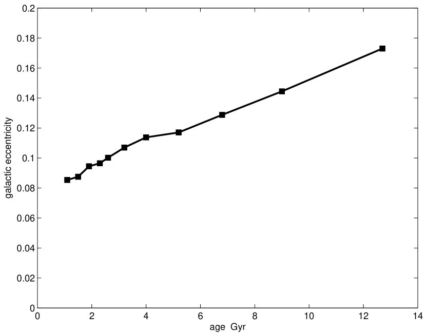
Figure 1: Dependence of mean orbital eccentricity on stellar age. Data extracted from the Geneva-Copenhagen spectroscopic survey of Hipparcos stars (Nordström et al., 2004).

The dynamic LSR is defined as a fictitious point currently at the position of the Sun in the Galactic plane, which moves along a perfectly circular orbit in a hypothetical axisymmetric potential. This definition is a mere theoretical concept, because the Galactic potential is not exactly axisymmetric, and there are no perfectly circular orbits. An alternative empirical definition of the LSR is the average motion of a sufficiently large, sufficiently homogeneous and sufficiently dynamically mixed sample of stars centered on the Sun. These two definitions are quite different, and in fact, are contradictory with regard to the shape of the reference orbit. Indeed, the empirical average reference orbit is markedly eccentric due to the stellar age-dependent asymmetric drift (see Fig. 1). The relative velocity of the Sun with respect to the empirical LSR is directly derived from our heliocentric astrometric observations, whereas determination of the solar peculiar velocity with respect to the hypothetical circular orbit is more involved (Mihalas & Binney, 1981; Dehnen & Binney, 1998) and relies on additional astrophysical or dynamical considerations.

If the Sun moves with a velocity $\vec{V}_{\sun}=(V_{X},V_{Y},V_{Z})$ relatively to the average motion of the local stars, the heliocentric velocity field of these stars contains a streaming motion in the opposite direction, that is, $-\vec{V}_{\sun}$. As far as tangential velocity components are concerned, this streaming motion is a dipolar vector field on the celestial sphere, and its exact representation via vector spherical harmonics (see Eqs. A) is

$$\vec{v}_{\tau}=V_{X}\vec{E}_{1}^{1}+V_{Y}\vec{E}_{1}^{-1}-V_{Z}\vec{E}_{1}^{0}.$$ (1)

Thus, the signature of the solar motion is confined to the first three electric harmonics only. We will see in the subsequent paragraphs that the other fundamental parameters of the velocity field are represented by magnetic harmonics and electric harmonics of higher degree, so that this effect is clearly separated in the vector harmonic space. It is worth noting that $\vec{V}_{\sun}$ is estimated from tangential velocities in physical units, i.e., from $\mu/\Pi$, where $\mu$ is the proper motion magnitude, and $\Pi$ is the parallax. A small admixture of halo stars and runaway stars with very high spatial velocities can perturb this determination.

We start with selecting $42\,487$ stars from the main Hipparcos catalog with statistically robust parallaxes ($\Pi/\sigma(\Pi)>5$) and without any indicators of binarity. To avoid extra-high velocity perturbers, we reject 148 stars with tangential velocities greater than 150 $\mbox{km\,s}^{-1}$  in either galactic component. A set of 24 vector harmonic functions is then fitted to the global vector field of $42\,339$ stars by a direct least-squares solution. The solar velocity components are simply read from the fitted coefficients of the first three electric harmonics. The results of this estimation are specified in Table 1, along with a sample of more distant stars with $\Pi>10$ mas ($24\,327$ stars).

The estimated velocity components $V_{X}$ and $V_{Z}$ are fairly similar for the two samples, indicating a negligible dependence on distance. They are also very close to the determination by Dehnen & Binney (1998). The estimates of $V_{Y}$ (in the direction of Galactic rotation) are very different between the two samples, beyond the possibility of a statistical fluke. The more distant stars move faster with respect to the Sun than the stars closer in. In either case, the stars move slower in this direction by more than 10 $\mbox{km\,s}^{-1}$  than the circular motion of the LSR determined by Dehnen & Binney (1998). This very prominent effect is attributed to the asymmetric drift of nearby stars, discussed in more detail in the next paragraph. Generally, there are three different reasons of physical and technical kind for our estimation of $V_{Y}$ to be biased:

1. the asymmetric drift;

2. the vertical gradient of rotational velocity $\Gamma(z)$;

3. the mixing of non-orthogonal harmonics.

3 The physical meaning of Oort’s constants

As long as a relatively small local area of the Galaxy around the Sun is considered ($r<<R_{0}$, where $R_{0}$ is the galactocentric distance of the Sun), it is appropriate to expand the systemic velocity field of stars in a Taylor series over the galactocentric cylindrical coordinates $(\rho,\theta,z)$. Assuming that the local field is planar, that is, all systemic motions are in the galactic plane, the velocity vector $\vec{v}(\rho,\theta,z)=\vec{a}(\rho,\theta)+\vec{\omega}(\rho,\theta,z)$, where the former component $\vec{a}$ is radial with respect to the Galactic center, and the latter, $\vec{\omega}$ is tangential and orthogonal to the former. Note that the radial component is assumed to be independent of $z$, that is, that there is no radial systemic motion depending on the distance from the plane. Retaining only first-degree terms in the corresponding Taylor expansion, one can write

$$a(\rho,\theta) = a_{0}+\delta\,(\rho-\rho_{0})+\epsilon\,\sin(\theta-\theta_{0})$$ (2)

$$\omega(\rho,\theta,z) = \omega_{0}+\alpha\,(\rho-\rho_{0})+\beta\,\sin(\theta-\theta_{0})+\Gamma(z)$$

where the subscript 0 denotes the corresponding parameters at the Sun’s location $(\rho_{0},\theta_{0},z_{0})$. We left the dependence of the rotational velocity $\omega$ on $z$ in its generic form, since on physical grounds, this dependence is expected to be symmetric around the plane, and can not be represented by a simple linear term.

Retaining only terms to $O(\frac{r}{\rho_{0}})$, these model relations can be rewritten more conveniently in the heliocentric coordinates $(r,\ell,b)$ introduced in Appendix A:

$$a(\vec{r}) = a_{0}-\delta\,r\cos\ell\,\cos b+\epsilon\,\frac{r}{\rho_{0}}\sin\ell\,\cos b$$ (3)

$$\omega(\vec{r}) = \omega_{0}-\alpha\,r\,\cos\ell\,\cos b+\beta\,\frac{r}{\rho_{0}}\sin\ell\,\cos b+\Gamma(z)$$

Apart from the reflex peculiar motion of the Sun treated in Section 2, we observe the heliocentric velocity field $\Delta\vec{v}=\vec{a}+\vec{\omega}-\vec{a}_{0}-\vec{\omega}_{0}$. Projections of this vector field onto the local tangential coordinate frames $(\vec{\tau}_{\ell},\vec{\tau}_{b})$ introduced in Appendix A, are

$$\Delta\vec{v}\cdot\vec{\tau}_{\ell} = \frac{\omega(\vec{r})}{2\rho_{0}}\,r\,\cos 2\ell\,\cos b-\frac{\omega(\vec{r})}{2\rho_{0}}\,r\,\cos b+(\omega(\vec{r})-\omega_{0})\,\cos\ell$$

$$+\frac{a(\vec{r})}{2\rho_{0}}\,r\,\sin 2\ell\,\cos b+(a(\vec{r})-a_{0})\,\sin\ell$$

$$\Delta\vec{v}\cdot\vec{\tau}_{b} = -\frac{\omega(\vec{r})}{2\rho_{0}}\,r\,\sin 2\ell\,\cos b\,\sin b-(\omega(\vec{r})-\omega_{0})\,\sin\ell\,\sin b$$

$$-\frac{a(\vec{r})}{2\rho_{0}}\,r\,\cos b\,\sin b+\frac{a(\vec{r})}{2\rho_{0}}\,r\,\cos 2\ell\,\cos b\,\sin b+(a(\vec{r})-a_{0})\,\cos\ell\,\sin b$$

Substituting the model (3) into Eqs. 3 and retaining only terms to $O(\frac{r}{\rho_{0}})$, we obtain after some toil the general expansion

$$\Delta\vec{v} = \left(\frac{\omega_{0}}{2\rho_{0}}-\frac{\alpha}{2}-\frac{\epsilon}{2\rho_{0}}\right)\,r\,\frac{1}{6}\,\vec{E}_{2}^{-2}+\left(-\frac{\omega_{0}}{2\rho_{0}}-\frac{\alpha}{2}+\frac{\epsilon}{2\rho_{0}}\right)\,r\,\vec{H}_{1}^{0}$$ (5)

$$+\left(\frac{a_{0}}{2\rho_{0}}-\frac{\delta}{2}-\frac{\beta}{2\rho_{0}}\right)\,r\,\frac{1}{6}\,\vec{E}_{2}^{2}+\left(-\frac{a_{0}}{2\rho_{0}}-\frac{\delta}{2}-\frac{\beta}{2\rho_{0}}\right)\,r\,\frac{1}{3}\,\vec{E}_{2}^{0}$$

$$+\frac{\Gamma(z)}{2\rho_{0}}\,r\,\frac{1}{6}\,\vec{E}_{2}^{-2}-\frac{\Gamma(z)}{2\rho_{0}}\,r\,\vec{H}_{1}^{0}-\Gamma(z)\,\vec{E}_{1}^{-1}$$

where we made use of the functional forms of the vector spherical harmonics in galactic coordinates specified in Appendix A. Disregarding for now the $\Gamma(z)$ terms, let us compare this equation with the classical expansion of the velocity field via the fundamental Oort’s constants (e.g., Torra et al., 2000), which in the vector harmonics notation takes the form

$$4.741\,r\,\vec{\mu}=A\cdot\frac{1}{6}\,\vec{E}_{2}^{-2}+B\cdot\vec{H}_{1}^{0}+C\cdot\frac{1}{6}\,\vec{E}_{2}^{2}-K\cdot\frac{1}{3}\,\vec{E}_{2}^{0}.$$ (6)

Hence, in our more general model, the Oort’s constants can be defined as

$$A = \frac{\omega_{0}}{2\rho_{0}}-\frac{\alpha}{2}-\frac{\epsilon}{2\rho_{0}}$$ (7)

$$B = -\frac{\omega_{0}}{2\rho_{0}}-\frac{\alpha}{2}+\frac{\epsilon}{2\rho_{0}}$$ (8)

$$C = \frac{a_{0}}{2\rho_{0}}-\frac{\delta}{2}-\frac{\beta}{2\rho_{0}}$$ (9)

$$K = \frac{a_{0}}{2\rho_{0}}+\frac{\delta}{2}+\frac{\beta}{2\rho_{0}}.$$ (10)

The slope of the local rotational velocity curve is readily derived as $\alpha=-(A+B)$. Since most of the recent and Hipparcos-based estimations arrive at $A\approx-B$, the rotation curve is locally almost (but not exactly) flat. It is also usually adopted that the local angular rotation velocity $\dot{\theta}_{0}$ is just the difference of the constants $A$ and $B$. In fact, however,

$$\dot{\theta}_{0}=\frac{\omega_{0}}{\rho_{0}}=A-B+\frac{\epsilon}{\rho_{0}}.$$ (11)

So, the local azimuthal shear of the radial motion $\epsilon$ contributes to the constants $A$ and $B$ and affect the determination of the angular velocity of the Galaxy. Presumably, this shear is small ($\epsilon<<\omega_{0}$), and our estimations are not hampered too much. The interpretation of the constants $C$ and $K$ is more complicated. Traditionally, the $C$ constant is called the shear, and the $K$ constant the local expansion (or dilation). In fact, we find that

$$C+K = \frac{a_{0}}{\rho_{0}}$$ (12)

$$K-C = \delta+\frac{\beta}{\rho_{0}}.$$ (13)

Presumably, there is no outward or inward bulk motion of stars around the Sun ($a_{0}=0$), and the LSR, empirically defined as the mean motion of a large homogenous heliocentric sample of stars, moves on a circular orbit. In numerous and somewhat conflicting determinations, it appears that, generally, $C\neq-K$, which indicates a nonzero systemic eccentricity of the local field. It is especially important in this case to accurately estimate the uncertainties of estimation, which may be larger than the estimates, as discussed in Section 4. The dilation is better characterized by the difference $K-C$ in Eq. 13, where $\delta$ can be interpreted as the radial heliocentric expansion, and $\beta/\rho_{0}$ as the azimuthal expansion. These two components can not be separated from proper motions alone.

4 Parameters of the velocity field

Using the vector harmonic formalism to describe the tangential velocity field on the celestial sphere (Appendix A) and the general expression for Ogorodnikov-Milne model (Eq. B5), makes the estimation of model parameters quite straightforward. The Hipparcos proper motions for our initial set of $42\,339$ non-binary stars with accurate parallaxes are converted to tangential velocities in the galactic coordinate system. Each velocity vector generates two condition equations, one for the longitudinal component $\vec{\tau}_{\ell}$ and the other for the latitudinal component $\vec{\tau}_{b}$. The coefficients of the expansion A2 are the unknowns of the condition equations, which are solved by the least-squares method. The main source of the solution uncertainty is the physical dispersion of individual velocity vectors related to peculiar orbital motions, since the astrometric errors of proper motions are small in the Hipparcos catalog, and the number of stars is large. The velocity dispersion is known to increase with age; it is also larger for thick disk stars than for thin disk stars. Instead of dealing with triaxial dispersion ellipsoids for various stellar populations, we take an empirical and robust approach to error estimation in this least-squares adjustment. We fit 24 vector harmonic functions up to degree 4 to the general vector field and consider this expansion to represent the systemic part of the velocity field. The residuals of the tangential velocity vectors represent the stochastic part of the field. Dispersions of velocities are computed from these residuals, separately for the $\vec{\tau}_{\ell}$ and $\vec{\tau}_{b}$ components, as half-differences between the 0.84 and 0.16 quantiles on each distribution. These quantities substitute standard deviation parameters for the markedly non-Gaussian velocity distributions. The resulting dispersions are $\sigma(v_{\ell})=24.0$ $\mbox{km\,s}^{-1}$, $\sigma(v_{b})=16.1$ $\mbox{km\,s}^{-1}$. The condition equations in longitude and in latitude are weighted with these quantities, respectively.

There are a few important technical notes to be made on this estimation problem. The solar peculiar velocity vector is determined directly from the tangential velocity field, expressed in units of $\mbox{km\,s}^{-1}$  (§2), in which case only the first three electric harmonics are of essence. The Oort or Ogorodnikov-Milne parameters describe a velocity field which grows linearly with distance from the Sun, and has distance $r$ in its functional form (B). The corresponding decomposition is done in the proper motion field, or, as we do it in this paper, the tangential velocities can be used in the observational part of the equations, but the harmonic functions are pre-multiplied with distances for each star. In the latter case, the distribution of sample stars on distance is taken into account automatically, and the harmonic coefficients have the desired dimension of $\mbox{km\,s}^{-1}$  kpc^-1. But before performing this distance-weighted least-squares estimation, the relative velocity of the Sun with respect to the stellar centroid should be subtracted for each star. This step proves to be of crucial importance because of the adverse effects of the harmonic leakage, discussed in § 4.1.

The results of vector harmonic estimation are specified in Table 2 for the original set of $42\,339$ stars, and for $24\,327$ stars more distant than 100 pc. All harmonic coefficients corresponding to Ogorodnikov-Milne parameters are shown, as well as other statistically significant coefficients which have no counterparts in the linear model. By statistically significant we conservatively mean a quantity larger than its formal error multiplied by $2.5$. Having the significance so defined we state that only three or four model OMM parameters are significant, and three extra non-linear parameters. The estimated parameters agree very well between the two sets, indicating no considerable dependence of the velocity field on distance within this fairly small volume. The slope of the rotation curve, using the results for the larger sample, is $\alpha=-(A+B)=-1.0\pm 1.8$ $\mbox{km\,s}^{-1}$  kpc^-1. This implies that the speed of rotation declines very slightly with galactocentric distance, but the conclusion is not reliable statistically. From Eq. 11, ignoring the possible contamination by the azimuthal shear $\epsilon$, the local angular rotation is $A-B=27.1\pm 1.8$ $\mbox{km\,s}^{-1}$  kpc^-1, in fine agreement with Feast & Whitelock (1997). Assuming a distance $\rho_{0}=7.9$ kpc for the Sun (see Vallée, 2005, and references therein), the speed of rotation is $\omega_{0}=214\pm 14$ $\mbox{km\,s}^{-1}$.

The $K$ constant is insignificant for both samples, but the $C$ constant is marginally significant, especially for more distant stars. The systemic outward motion $a_{0}=\rho_{0}(C+K)$ appears to be negligible for the general sample, but the more distant stars seem to exhibit an inward motion of $a_{0}=-42\pm 20$ $\mbox{km\,s}^{-1}$. This result is qualitatively consistent with the estimation by Hanson (1987) who found a progressively smaller solar velocity toward the Galactic center with respect to stars at higher latitudes. If this inward motion in the outer part of the astrometrically known Galaxy is real, it may be somewhat counterbalanced by the small but persistent dilation (expansion) of the local stellar aggregate, at $K-C\simeq 4\pm 2$ $\mbox{km\,s}^{-1}$  kpc^-1. Associations of young stars expand by virtue of their initial velocity dispersions (Makarov et al., 2004), and the presence of the young Local Association could be invoked to explain the local expansion. It is worth emphasizing that the accuracy of the available astrometric data on the local stellar field is still insufficient to establish these subtle effects with certainty. In fact, the barely noticeable $K$ and $C$ constants may be related to the intermediate-scale streams of stars permeating the solar neighborhood, rather than to the general pattern of Galactic rotation. Famaey et al. (2005) present a scrutiny of such streams or superclusters, based on the best available radial velocity and astrometry data for K and M giants, including the Hyades, Sirius, Hercules and B streams. Apart from strong evidence for asymmetric drift for evolved stars, they find, interestingly, that the centroid velocity of the Sun $V_{X}$ with respect to giants is $\simeq 10$ $\mbox{km\,s}^{-1}$, in agreement with our present and other previous estimations, but it drops to only $\simeq 3$ $\mbox{km\,s}^{-1}$  when all the major streams are excluded. This difference may be interpreted as a net outward radial motion of the streams (see also their Table 1). Famaey et al. (2005) point out that the members of these streams have a spread of ages and other physical characteristics, and the streams must be dynamically induced. The authors raise the question of how the standard solar motion can actually be defined if the motion of even the oldest and supposedly dynamically mixed stellar populations is subject to unknown dynamical agents perturbing their orbits? We think that the stellar streams are legitimate parts of the local velocity field, and that it makes sense to define the velocity centroid and the solar peculiar motion in much the same way as it has been done before, keeping in mind that dynamical mixing and relaxation may be a mere theoretical idealization, as well as a circularly moving LSR.

4.1 Harmonic leakage

As specified in Table 2, we find only three significant terms in the general vector harmonic decomposition beyond the Ogorodnikov-Milne model, viz., $H_{2}^{-1}$, $E_{3}^{-1}$, and $E_{4}^{2}$. All other estimated harmonics, including all third and fourth degree terms, are well below $2.5\sigma$. Thus, we find little evidence of nonlinear patterns in the motion of local stars. The actual velocity field progressively deviates from the linear approximation of the model with heliocentric distance. Furthermore, the rotation curve may have local wiggles and curvature, as discussed in Olling & Merrifield (1998). One way of tackling this problem is to build a more complex model in which the Oort’s constants are actually functions of coordinates, to be determined from observations. We take a different approach in this paper, determining empirically a vector harmonic decomposition and trying to interpret those terms that appear to be statistically significant.

Before embarking on analysis of the emerging nonlinear harmonics (and the unexpected linear term $H_{1}^{-1}$), we should examine a technical, but crucial problem in the determination of model parameters. The stellar velocity field bears a strong signal in the classical terms representing the reflex solar motion and the Oort’s constants $A$ and $B$. These terms are represented in our model by specific vector harmonics (Appendix B). The strong signal in the physically meaningful low-degree harmonics in the velocity space can leak into higher-degree vector harmonics in the proper motion space, resulting in spurious detections of nonlinear effects. This inevitably happens because the sampled vector harmonics are not independent for any inhomogeneous discrete set of points. This problem has two somewhat different aspects. In classical applications, when only proper motions are known from observation, the mean parallax of nearby stars varies across the sky because of the real clumps in number density (the Gould Belt, large associations, spiral arms), as well as the non-uniform interstellar extinction. This difficulty was first spotted by Edmondson (1937), and later investigated in more detail by Olling & Dehnen (2003). In the latter paper, a nice example is presented, how the longitudinal variation of the mean parallax, described by a Fourier series, makes the simple dipolar pattern of the solar motion to contribute to the terms that would be empirically defined as the $A$ and $B$ constants. Our analysis is free of this complication, because we use accurate trigonometric parallaxes from the Hipparcos catalog, and perform the estimations of the solar motion in the velocity space, and of model parameters separately in the proper motion space. But there is another, more basic reason to be concerned about the harmonic leakage. The lack of uniformity in the number density of stars on the sky itself makes the vector harmonics mutually dependent within either coordinate component.

Mathematically, the problem can be viewed as a lack of orthogonality of the sampled harmonics. The degree of non-orthogonality is quantified by the correlation coefficients readily computed from the off-diagonal elements of the covariance matrix. For our nearby stars, the largest physical effect is the solar motion expressed by the first-degree electric harmonics, and the cross-talk of these terms with other harmonics of higher degree may generate false positive detections.

We set up a dedicated numerical experiment to prove that this contamination may happen unless appropriate precautions are taken. We use the same general set of Hipparcos stars as before, but the actual observed proper motions are replaced with simulated vectors, computed from the reflex solar motion only, estimated in §2. A harmonic decomposition of the simulated velocity field produces the same velocity dipole in the first electric harmonics, and zero for the rest of harmonics, which only shows that the software works correctly. But when a similar decomposition is carried out in the space of distance-weighted harmonics, as described in §4, a number of spurious terms emerge, viz., $\vec{H}_{2}^{-1}$ (significance level $8.8\sigma$), $\vec{H}_{2}^{0}$ ($5.4\sigma$), $\vec{H}_{2}^{2}$ ($3.2\sigma$), $\vec{E}_{3}^{-3}$ ($8.9\sigma$), $\vec{E}_{3}^{-1}$ ($4.0\sigma$), $\vec{E}_{3}^{0}$ ($7.6\sigma$), $\vec{E}_{3}^{2}$ ($8.7\sigma$), and $\vec{E}_{3}^{3}$ ($3.8\sigma$). The appearance of the $\vec{H}_{2}^{-1}$ and $\vec{E}_{3}^{-1}$ harmonics is especially worrisome, because they may carry some physical information, as discussed in subsequent paragraphs. The simplest way to get rid of most of the harmonic leakage effect is to subtract the reflex solar motion from all tangential velocities prior to a model parameter fitting. Ideally this eliminates the perturbations from the dominating dipolar terms. Note that existing correlations between the sampled distance-weighted vector harmonics that we use to determine OMM parameters, do not affect the results in a systematic way, because the least-squares solution is unbiased. The major adverse effect of these correlations is an enhanced propagation of random and possibly systematic errors from our observational data.

5 Vertical gradient of rotational velocity

The apparent relative velocity of the Sun in the direction of galactic rotation ($V_{Y\sun}$) varies with distance of reference field stars from the Galactic plane. This remarkable fact was established by Hanson (1989) from proper motions of fairly distant stars, and recently confirmed by Girard et al. (2006), who used absolute proper motions of giant stars in the direction of south Galactic pole. The thick disk dominates between $z=1$ and $3$ kpc, where the rotational lag of field stars is found to follow a nearly linear dependence on vertical height, accompanied, predictably, by a growth of velocity dispersion in the $X$ direction. The slope of the lag, from both cited papers, is estimated at $-30$ $\mbox{km\,s}^{-1}\,\mbox{kpc}^{-1}$. Girard et al. also offer a dynamical interpretation of this phenomenon, finding it consistent with a general model of the Galactic potential. The sample of nearby Hipparcos stars considered in this paper is practically limited to 200 pc, and is dominated by thin disk stars. Is there a similar vertical gradient of rotational velocity for the thin disk?

Evidently from Eq. A2, a vertical lag affects the determination of the centroid velocity $V_{Y}$ expressed by the dipole vector harmonic $\vec{E}_{1}^{-1}$, because $\Gamma(z)$ is negative everywhere except $z=0$. If the velocity of rotation falls off with increasing $z$, the relative solar velocity $V_{Y\sun}$ should grow with distance due to the admixture of high-$z$ stars. This is not what we find in Table 1, where the more distant stars ($\Pi<10$ mas) appear to rotate faster than the overall sample of stars. However, a more accurate consideration reveals that for a number of possible functional forms of $\Gamma(z)$ (e.g., $\Gamma\cdot|z|$, $\Gamma\cdot|z|^{2}$), the most characteristic response is expected in the $\vec{E}_{3}^{-1}$ harmonic, because the $\vec{E}_{1}^{-1}$ harmonic is too sensitive to the choice of centroid solar motion. Our choice of velocity in Table 1, consistent with the estimation for the more distant half of Hipparcos stars, is justified by the fact that the OMM parameters are determined in the distance-weighted (or proper motion) space where distant stars are more significant, and whatever kinematics anomalies the nearest stars may have, has little bearing on the OMM estimation problem. The rotation gradient dipole $\vec{E}_{1}^{-1}$ emerges with a robust positive coefficient $e_{1}^{-1}=11.25\pm 1.17$ $\mbox{km\,s}^{-1}\,\mbox{kpc}^{-1}$, which is consistent with a negative gradient of $\Gamma(z)$.

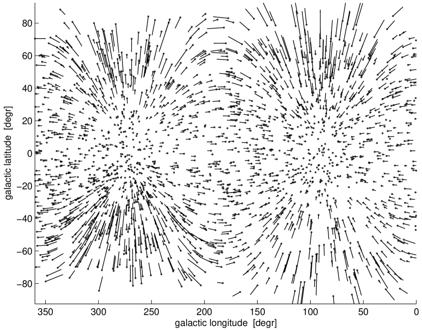
Figure 2: The velocity field of Hipparcos stars generated by the vertical gradient of rotational velocity.

We performed direct simulations of the vector harmonic response to a linear gradient $\Gamma(z)=\Gamma\cdot|z|$ for different values of $\Gamma$ and the height of the Sun above the plane $z_{\sun}$. A good match with observations was found for $\Gamma=-20$ $\mbox{km\,s}^{-1}\,\mbox{kpc}^{-1}$and $z_{\sun}=15$ pc, which yielded a set of coefficients $e_{1}^{-1}=11.41\pm 1.17$, $h_{2}^{1}=-2.04\pm 0.47$, and $e_{3}^{-1}=0.75\pm 0.22$ $\mbox{km\,s}^{-1}\,\mbox{kpc}^{-1}$, all the rest 21 harmonics being insignificant. Both electric harmonics are in good agreement with our fit for all star, whereas the $h_{2}^{1}$ coefficient is fairly close to the fit ($-1.09\pm 0.47$, not shown in Table 2). Therefore, a linear gradient of rotational velocity of the thin disk of roughly $-20$ $\mbox{km\,s}^{-1}\,\mbox{kpc}^{-1}$is a plausible explanation to the corresponding set of vector harmonic terms beyond the Ogorodnikov-Milne model. The detected pattern of tangential velocities of Hipparcos stars consistent with this interpretation is shown in Fig. 2.

6 Warp and the origin of $\vec{H}_{1}^{-1}$ and $\vec{H}_{2}^{-1}$

The Milky Way disk is warped, as has been established from the distribution of stars and neutral hydrogen. In this respect, our Galaxy is not different from many other spiral galaxies exhibiting a range of warp distortions. The origin of galactic warps is not clear; a number of hypotheses have been proposed, including the tidal interaction of the disk with the dark matter halo, the influence of the bar, and the perturbation from a major satellite galaxy. The Sun appears to be close to the line of nodes of the Milky Way warp, and the upper rim of the disk is at $\ell=90\arcdeg$ (in the rotation direction). The height of the midsection above the plane is quadratic with galactocentric distance in the model of Drimmel et al. (2000), $w(\rho)=(\rho-\rho_{w})^{2}/15$ kpc for $\rho>\rho_{w}$, and zero for $\rho<\rho_{w}$. According to Momany et al. (2006), the warp begins well within the solar circle ($\rho_{w}<\rho_{\sun}$), and the line of nodes deviates from the solar radius by $15\arcdeg$.

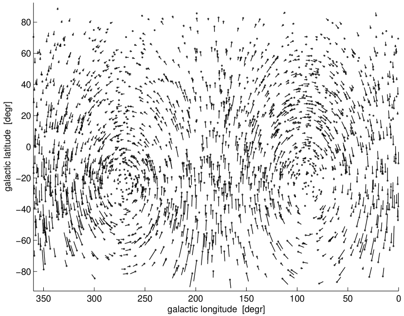
Figure 3: The velocity field of Hipparcos stars generated by the two unexpected magnetic vector harmonics, $\vec{H}_{1}^{-1}$ and $\vec{H}_{2}^{-1}$.

The single most unexpected result of our analysis is the strong model parameter $L_{13}$ (Table 2), represented by the coefficient of the first-degree magnetic harmonic $\vec{H}_{1}^{-1}$, that is, a rigid rotation around the direction $-Y$ (see Eqs. A). The sign of this parameter implies that the stars move upward in the direction of the Galactic center, downward in the opposite direction, away from the center at the north pole, and toward the center at the south pole. The signal-to-noise ratio on this parameter is about 6. The extra statistically significant term $h_{2}^{-1}$ detected by us in the local velocity field may be related to the former. The pattern of tangential velocities generated by these two magnetic harmonics, $6.21\,r\vec{H}_{1}^{-1}-1.20\,r\vec{H}_{2}^{-1}$, is shown in Fig. 3. The main effect of the higher degree harmonic is that the axis of rotation lies below the plane at roughly $b=-20\arcdeg$, nearly obliterating the motion in the north pole region, but retaining the galactocentric motion near the south pole. The most conspicuous features are the general upward motion of stars in the direction of the galactic center, and the downward motion of stars at $\ell=180\arcdeg$. It is tempting to relate these two unexpected components to a kinematic signature of the Galactic warp.

The shape of the warp, as traced by the distribution of neutral hydrogen and dust, implies that the stars in the solar region are involved in a general upward motion, since the starting rim of the warp is within the solar circle ($\rho_{w}=6.5$ kpc). This common motion is indistinguishable from the vertical solar reflex motion, but the model also implies a radial gradient of the upward velocity, $V_{Z,{\rm warp}}\propto(\rho-\rho_{w})$, which is detectable in the proper motion field. In the near-plane zone, the differential warp motion manifests itself as a downward stream at $\ell\approx 0$, and an upward stream at $\ell\approx 180\arcdeg$. Obviously, the pattern in Fig. 3 is completely inconsistent with this prediction. Assuming for simplicity that the Sun lies on the line of nodes, the linear Taylor expansion of the local velocity field (2) should be expanded to include a vertical ($Z$) component of velocity,

$$\lambda(\rho)=\lambda_{0}+\Lambda(\rho-\rho_{0})\approx\lambda_{0}-\Lambda\,r\,\cos\ell\cos b.$$ (14)

The corresponding tangential velocity field is

$$\Delta\vec{v}_{\tau}=-\Lambda\,r\,\cos\ell\cos^{2}b\,\tau_{b}=-\Lambda\,r\,(\frac{1}{2}\vec{H}_{1}^{-1}-\frac{1}{6}\vec{E}_{2}^{1}).$$ (15)

Thus, the differential warp motion is expressed by two OMM parameters, $L_{13}$ and $M_{13}$. These two fitted parameters yield discrepant estimates of the warp velocity gradient, $\Lambda=-2\,h_{1}^{-1}\simeq-12$ $\mbox{km\,s}^{-1}\,\mbox{kpc}^{-1}$, and $\Lambda=6\,e_{2}^{1}\simeq+4$ $\mbox{km\,s}^{-1}\,\mbox{kpc}^{-1}$. The former estimate from the magnetic harmonic has the wrong sign, and its modulus is too large for a credible differential warp. The electric harmonic $\vec{E}_{2}^{1}$ has the right sign, but it nearly vanishes for more distant stars ($\Pi<10$ mas). Thus, the kinematical model of Galactic warp does not furnish an adequate explanation to the presence of magnetic harmonics $\vec{H}_{1}^{-1}$ and $\vec{H}_{2}^{-1}$. Samples of larger volumes are needed to find out if these two harmonics are not a local feature, and to find evidence of warp in the motion of field stars. Interestingly, Drimmel et al. (2000) also found a negative vertical motion of distant OB stars in the direction of Galactic anticenter, in obvious contradiction to the predicted warp motion. A non-stationary warp is one of the possibilities considered by them. A precessing line of nodes is conceivable, but we find it difficult to reconcile the observed pattern of vertical motion, should it bear on the subject at all, with a plausible precession model. It appears instead, that the line of nodes is stationary, but the shape of warp changes to its opposite every 50 Myr or so, curling this way and the other.

7 Conclusions and Back to Astrometry

Hipparcos stars with accurate trigonometric parallaxes represent only a tiny fraction of the Galactic population. Half of stars considered in this paper are within 112 pc, and 75 % are within 160 pc. The narrow horizon of our selection limits the accuracy of vector harmonic terms describing the local tangential velocity field in the most general and systematic fashion. Only several major kinematical parameters can be determined with confidence from such a limited data set. We determine the relative solar velocity with respect to all stars in our selection, and to stars with measured distances greater than 100 pc. The latter determination yields $V_{\sun}=(9.9,15.6,6.9)\pm 0.2$ $\mbox{km\,s}^{-1}$, which we add to the tangential velocities of all field stars before performing a general decomposition of the velocity field onto vector spherical harmonics. This decomposition provides values of $A=13.8\pm 1.4$ and $B=-13.4\pm 1.2$ $\mbox{km\,s}^{-1}\,\mbox{kpc}^{-1}$  for the fundamental Oort’s constants of differential galactic rotation. Since $A+B\approx 0$, the local rotation velocity curve is nearly flat. Assuming a galactocentric distance of 7.5 kpc for the Sun, a rotation velocity of $\omega_{0}=204\cdot[\rho_{0}/7.5\;{\rm kpc}]$ $\mbox{km\,s}^{-1}$  is derived.

Among other linear OMM parameters, we detect, most unexpectedly, a strong signal carried by the first-degree magnetic harmonic $\vec{H}_{1}^{-1}$, which describes a rigid rotation of the stellar field around the axis $-Y$ opposite to the direction of galactic rotation. The estimated rate of this rotation is roughly 6 $\mbox{km\,s}^{-1}\,\mbox{kpc}^{-1}$, or 1.3 $\mbox{ mas\,yr}^{-1}$  in proper motions along the principal galactic meridian. Another unexpected magnetic harmonic, $\vec{H}_{2}^{-1}$, nearly cancels out the outward motion at the North pole predicated by the former harmonic, but retains the strong inward motion around the South pole, and the counter vertical motions near the Galactic plane. Differential vertical velocities naturally arise from a kinematic model of the Galactic warp, but we find that the sign of the local rotation is opposite to what is required to raise the rim of the Galaxy above the plane in the first and second quadrants. In other words, the local stars are expected to move upwards due to the warp, but we detect a negative differential rotation. Analysis of velocity fields in a much larger volume of space is needed to make sure that this discordant rotation is not a local feature, which would have crucial consequences for our understanding of the physics of the warp.

Only three statistically significant vector harmonic terms beyond the Ogorodnikov-Milne model are detected in this paper. One of them, the electric multipole $\vec{E}_{3}^{-1}$, is of special note, since, together with a positive residual dipole $\vec{E}_{1}^{-1}$ in the direction of galactic rotation, it is likely to advertise a vertical gradient of rotation velocity. A similar gradient of rotational lag of $-30$ $\mbox{km\,s}^{-1}\,\mbox{kpc}^{-1}$  has been found in proper motions of more distant stars representing the thick disk population, but never reported for the thin disk dominating our sample. We estimate a gradient of $\simeq-20$ $\mbox{km\,s}^{-1}\,\mbox{kpc}^{-1}$  for our sample of nearby stars limited to 200 pc. This result requires verification on a larger sample of thin disk stars extending to 1 kpc.

Our concluding remark is that estimation of subtle effects in the local kinematics pertaining to the Galactic structure and formation history is based on the assumption that the Hipparcos proper motion data is free of large-scale systematic errors at $\gtrsim 1$ $\mbox{ mas\,yr}^{-1}$. None such errors have been reported in the literature, which is not a strong argument because Hipparcos remains unparalleled at its level of global astrometric accuracy. The major catalogs of proper motions Tycho-2 (Urban et al., 2000) and UCAC (Zacharias et al., 2004) are calibrated on Hipparcos stars; therefore, systematic distortions of Hipparcos astrometry, if any, are just copied over to these catalogs. Radio astrometric observations with VLBI have recently advanced to a comparable level of accuracy in positions and proper motions, and being directly tied to the ICRF, provide an independent test for the Hipparcos reference system (Boboltz et al., 2006). This important external check is unfortunately limited by the small number of optically bright radio stars, but the available accuracy of VLBI proper motions (approximately $1.7$ $\mbox{ mas\,yr}^{-1}$) enables Boboltz et al. to state that the relative spin of the Hipparcos proper motion system is much less than 1 $\mbox{ mas\,yr}^{-1}$  about each axis. This result confirms that the strong magnetic harmonic $\vec{H}_{1}^{-1}$ representing a spin around the $-Y$ direction, is not an artefact. Another significant astrometric development of late is the SPM3 catalog, which provides high quality absolute proper motions for a large sample of distant and faint stars, albeit in a small fraction of the sky (Girard et al., 2004). This catalog provides an independent view of the local stellar velocity field in the surveyed area of the sky.

Appendix A Vector spherical harmonic decomposition of a proper motion field

As customary in studies of Galactic dynamics, we make use of the Galactic coordinate system $(X,Y,Z)$ in which the $X$ axis is pointing toward the Galactic center, the $Y$ axis toward the direction of Galactic rotation, and the $Z$ axis toward the north pole. For each star, a triad of unit vectors $(\vec{r},\vec{\tau_{l}},\vec{\tau_{b}})$ is defined, with

$$\vec{\tau}_{r}=\left(\begin{array}[]{c}\cos\ell\cos b\\ \sin\ell\cos b\\ \sin b\end{array}\right)\hskip 11.38109pt\vec{\tau}_{\ell}=\left(\begin{array}[]{c}-\sin\ell\\ \cos\ell\\ 0\end{array}\right)\hskip 11.38109pt\vec{\tau}_{b}=\left(\begin{array}[]{c}-\cos\ell\sin b\\ -\sin\ell\sin b\\ \cos b\end{array}\right),$$ (A1)

where $\tau_{\ell}$ and $\tau_{b}$ define the tangential coordinate directions toward increasing galactic longitude $\ell$ and the north pole, respectively. The proper motion vector of the object is traditionally projected onto the locally tangential coordinate vectors, that is, $\vec{\mu}=\mu_{\ell}\cos b\,\vec{\tau_{\ell}}+\mu_{b}\,\vec{\tau_{b}}$.

A global proper motion field of a large set of celestial objects can be represented by the expansion

$$\vec{\mu}(\ell,b)=\sum_{n=1}^{\infty}\sum_{m=-n}^{n}[h_{n}^{m}\vec{H_{n}^{m}}(\ell,b)+e_{n}^{m}\vec{E_{n}^{m}}(\ell,b)],$$ (A2)

where $\ell$ and $b$ are galactic longitudes and latitudes, $\vec{H_{n}^{m}}$ and $\vec{E_{n}^{m}}$ are orthogonal vector harmonics which we call magnetic and electric vector harmonics respectively. These vector harmonics are derived via partial derivatives of the scalar spherical harmonics over angular coordinates, viz.:

$$\vec{H_{n}^{m}}(\ell,b) = \left[\frac{\partial S_{n}^{m}(\ell,b)}{\partial b}\vec{\tau_{\ell}}-\frac{1}{\cos b}\frac{\partial S_{n}^{m}(\ell,b)}{\partial\ell}\vec{\tau_{b}}\right]$$

$$\vec{E_{n}^{m}}(\ell,b) = \left[\frac{1}{\cos b}\frac{\partial S_{n}^{m}(\ell,b)}{\partial\ell}\vec{\tau_{\ell}}+\frac{\partial S_{n}^{m}(\ell,b)}{\partial b}\vec{\tau_{b}}\right]$$ (A3)

Spherical harmonics $S_{n}^{m}$ are counted by degrees $n=0,1,\ldots$ and orders $m=-n,-n+1,\ldots,n$. Explicitly,

$$S_{n}^{m} = \sqrt{\frac{2n+1}{2\pi}\frac{(n-m)!}{(n+m)!}}P_{n}^{m}(\sin b)\cos m\ell,\hskip 22.76219ptm>0,$$ (A4)

$$= \sqrt{\frac{2n+1}{4\pi}}P_{n}^{0}(\sin b)\hskip 113.81102ptm=0,$$

$$= \sqrt{\frac{2n+1}{2\pi}\frac{(n-|m|)!}{(n+|m|)!}}P_{n}^{|m|}(\sin b)\sin|m|\ell,\hskip 11.38109ptm<0$$

where $P_{n}^{m}$ are the associated Legendre polynomials. The first pair of vector harmonics are generated by from the scalar zonal harmonic $S_{1}^{0}$, with the electric component $\cos b\vec{\tau}_{b}$ and the magnetic component $\cos b\vec{\tau}_{\ell}$. The electric vector harmonics for $n<=2$ in angular coordinates are

$$\vec{E}_{1}^{-1} = -\cos\ell\,\vec{\tau_{\ell}}+\sin\ell\sin b\,\vec{\tau_{b}}$$

$$\vec{E}_{1}^{0} = \cos b\,\vec{\tau_{b}}$$

$$\vec{E}_{1}^{1} = \sin\ell\,\vec{\tau_{\ell}}+\cos\ell\sin b\,\vec{\tau_{b}}$$

$$\vec{E}_{2}^{-2} = 6\cos 2\ell\,\cos b\,\vec{\tau_{\ell}}-6\sin 2\ell\,\cos b\,\sin b\,\vec{\tau_{b}}$$

$$\vec{E}_{2}^{-1} = -3\cos\ell\,\sin b\,\vec{\tau_{\ell}}-3\sin\ell\cos 2b\,\vec{\tau_{b}}$$

$$\vec{E}_{2}^{0} = 3\cos b\,\sin b\,\vec{\tau_{b}}$$

$$\vec{E}_{2}^{1} = 3\sin\ell\,\sin b\,\vec{\tau_{\ell}}-3\cos\ell\,\cos 2b\,\vec{\tau_{b}}$$

$$\vec{E}_{2}^{2} = -6\sin 2\ell\,\cos b\,\vec{\tau_{\ell}}-6\cos 2\ell\,\cos b\,\sin b\,\vec{\tau_{b}},$$ (A6)

and the magnetic vector harmonics for $n<=2$ are

$$\vec{H}_{1}^{-1} = \sin\ell\,\sin b\,\vec{\tau_{\ell}}+\cos\ell\,\vec{\tau_{b}}$$

$$\vec{H}_{1}^{0} = \cos b\,\vec{\tau_{\ell}}$$

$$\vec{H}_{1}^{1} = \cos\ell\,\sin b\,\vec{\tau_{\ell}}-\sin\ell\,\vec{\tau_{b}}$$

$$\vec{H}_{2}^{-2} = -6\sin 2\ell\,\cos b\,\sin b\,\vec{\tau_{\ell}}-6\cos 2\ell\,\cos b\,\vec{\tau_{b}}$$

$$\vec{H}_{2}^{-1} = -3\sin\ell\,\cos 2b\,\vec{\tau_{\ell}}+3\cos\ell\sin b\,\vec{\tau_{b}}$$

$$\vec{H}_{2}^{0} = 3\cos b\,\sin b\,\vec{\tau_{\ell}}$$

$$\vec{H}_{2}^{1} = -3\cos\ell\,\cos 2b\,\vec{\tau_{\ell}}-3\sin\ell\,\sin b\,\vec{\tau_{b}}$$

$$\vec{H}_{2}^{2} = -6\cos 2\ell\,\cos b\,\sin b\,\vec{\tau_{\ell}}+6\sin 2\ell\,\cos b\,\vec{\tau_{b}},$$ (A7)

Note that the normalization coefficients of the generic spherical harmonics (A4) are omitted in these formulas.

Appendix B Ogorodnikov-Milne model via vector harmonics formalism

The linear Ogorodnikov-Milne model of the local velocity field in its general matrix form can be written as (du Mont, 1977)

$$\vec{V}=\left(\begin{array}[]{ccc}M_{11}&M_{12}&M_{13}\\ M_{12}&M_{22}&M_{23}\\ M_{13}&M_{23}&M_{33}\end{array}\right)\vec{r}+\left(\begin{array}[]{ccc}0&-L_{12}&-L_{13}\\ L_{12}&0&-L_{23}\\ L_{13}&L_{23}&0\end{array}\right)\vec{r},$$ (B1)

where $\vec{V}$ is the systemic part of the velocity field as a function of the position vector $\vec{r}$. It is assumed in the following that positions are determined with respect to the solar system barycenter; any shift of the coordinate system origin results in an additional constant translation term. For convenience, the matrix of transformation is split into the symmetric (shear) part $M$ and the antisymmetric traceless (rotation) part $L$. It is readily seen that the matrix $M$ describes the gradient-type distortions of the field, and the $L$ part represents rigid rotations, or spins, around the three coordinate axes.

After a small manipulation, the tangential velocity components are

$$V_{l}/r=(\vec{V}\cdot\vec{\tau}_{\ell})/r = (-M_{11}+M_{22})\sin\ell\cos\ell\cos b+M_{12}\cos 2\ell\cos b$$

$$-M_{13}\sin\ell\sin b+M_{23}\cos\ell\sin b+L_{12}\cos b+L_{13}\sin\ell\sin b-L_{23}\cos\ell\sin b$$

$$V_{b}/r=(\vec{V}\cdot\vec{\tau}_{b})/r = (-M_{11}\cos^{2}\ell-M_{22}\sin^{2}\ell+M_{33})\sin b\cos b-M_{12}\sin 2\ell\sin b\cos b$$

$$+M_{13}\cos\ell\cos 2b+M_{23}\sin\ell\cos 2b+L_{13}\cos\ell+L_{23}\sin\ell$$

Comparing these equations with the trigonometric expressions for low-degree vector spherical harmonics (Appendix A), the following relations of proportionality are established

$$M_{12} \propto e_{2}^{-2}$$

$$M_{23} \propto -e_{2}^{-1}$$

$$M_{13} \propto -e_{2}^{1}$$

$$D_{1} \propto e_{2}^{2}$$

$$D_{2} \propto e_{2}^{0}$$

$$L_{12} \propto h_{1}^{0}$$

$$L_{13} \propto h_{1}^{-1}$$

$$L_{23} \propto -h_{1}^{1},$$ (B2)

where

$$D_{1}=\frac{1}{2}(M_{11}-M_{22});\hskip 11.38109ptD_{2}=M_{33}+\frac{1}{2}(M_{11}+M_{22}).$$ (B3)

Clearly, all nine parameters of the Ogorodnikov-Milne model can not be determined from a proper motion field, since an isotropic dilation ($M_{11}=M_{22}=M_{33}$) results in radial velocities only. This is why only eight parameters of the model appear in the vector harmonic decomposition of a proper motion field (Vityazev & Shuksto, 2004).

We further establish the relations between the constants of the Ogorodnikov-Milne model and the four constants ($A,B,C,K$) of the Oort’s two-dimensional model by matching the terms in the proper motion equation of the latter (Torra et al., 2000)

$$4.741\,\vec{\mu} = (A\cos 2\ell\cos b+B\cos b-C\sin 2\ell\cos b)\,\vec{\tau}_{\ell}$$ (B4)

$$+(-A\sin 2l\ell\sin b\cos b-C\cos 2\ell\sin b\cos b-K\sin b\cos b)\,\vec{\tau}_{b}.$$

The corresponding equation for the more general Ogorodnikov-Milne model in terms of vector harmonics is

$$4.741\,\vec{\mu} = L_{13}\vec{H}_{1}^{-1}+L_{12}\vec{H}_{1}^{0}-L_{23}\vec{H}_{1}^{1}$$ (B5)

$$+\frac{1}{6}M_{12}\vec{E}_{2}^{-2}-\frac{1}{3}M_{23}\vec{E}_{2}^{-1}-\frac{1}{3}D_{2}\vec{E}_{2}^{0}-\frac{1}{3}M_{13}\vec{E}_{2}^{1}+\frac{1}{6}D_{1}\vec{E}_{2}^{2},$$

where $M_{12}=A$, $L_{12}=B$, $D_{1}=C$ and $D_{2}=K$.

Table 1: Determination of the centroid velocity of the Sun

component	$\Pi<10$ mas	all stars
$V_{X}=e_{1}^{1}$	$9.9\pm 0.2$	$10.5\pm 0.1$
$V_{Y}=e_{1}^{-1}$	$15.6\pm 0.2$	$18.5\pm 0.1$
$V_{Z}=-e_{1}^{0}$	$6.9\pm 0.2$	$7.3\pm 0.1$

Table 2: Determination of Ogorodnikov-Milne and higher degree parameters of the local velocity field

	$\Pi<10$ mas	all stars
$L_{13}=h_{1}^{-1}$	$5.91\pm 1.02\;(5.8)$	$6.21\pm 0.94\;(6.6)$
$L_{12}=B=h_{1}^{0}$	$-12.36\pm 1.26\;(9.8)$	$-13.36\pm 1.16\;(11.5)$
$L_{23}=-h_{1}^{1}$	$0.13\pm 0.97\;(0.1)$	$-0.36\pm 0.89\;(0.4)$
$M_{12}=A=6\,e_{2}^{-2}$	$14.08\pm 1.56\;(9.2)$	$13.83\pm 1.42\;(9.8)$
$M_{23}=-3\,e_{2}^{-1}$	$0.38\pm 1.37\;(0.3)$	$0.76\pm 1.25\;(0.6)$
$X_{2}=K=-3\,e_{2}^{0}$	$-0.63\pm 1.98\;(0.3)$	$1.02\pm 1.81\;(0.6)$
$M_{13}=-3\,e_{2}^{1}$	$-0.32\pm 1.38\;(0.2)$	$-2.13\pm 1.27\;(1.7)$
$X_{1}=C=6\,e_{2}^{2}$	$-4.72\pm 1.64\;(3.1)$	$-3.03\pm 1.43\;(2.1)$
Other significant parameters
$e_{1}^{-1}$	$-0.81\pm 1.28\;(0.6)$	$11.25\pm 1.17\;(9.6)$
$h_{2}^{-1}$	$-1.69\pm 0.44\;(3.8)$	$-1.20\pm 0.41\;(2.9)$
$e_{3}^{-1}$	$0.52\pm 0.24\;(2.2)$	$0.80\pm 0.22\;(3.7)$
$e_{4}^{2}$	$-0.075\pm 0.041\;(1.9)$	$-0.100\pm 0.037\;(2.7)$

Note. — All parameters and their formal standard errors are specified in $\mbox{km\,s}^{-1}\,\mbox{kpc}^{-1}$; the signal-to-noise ratio is given in brackets. A solar velocity $V_{\sun}=(9.9,15.6,6.9)$ $\mbox{km\,s}^{-1}$  was subtracted for both sets of stars.

References

- Binney & Tremaine (1987) Binney, J.J., Tremaine, S. 1987, Galactic Dynamics, Princeton Univ. Press, Princeton, NJ
- Boboltz et al. (2006) Boboltz, D.A., et al. 2006, AJ, in print
- ESA (1997) ESA, 1997, The Hipparcos Catalogue. ESA SP-1200
- du Mont (1977) du Mont, B. 1977, A&A, 61, 127
- Dehnen & Binney (1998) Dehnen, W., & Binney, J.J. 1998, MNRAS, 298, 387
- Drimmel et al. (2000) Drimmel, R., Smart, R.L., Lattanzi, M.G. 2000, A&A, 354, 67
- Edmondson (1937) Edmondson, F.K. 1937, MNRAS, 97, 473
- Famaey et al. (2005) Famaey, B., et al. 2005, A&A, 430, 165
- Feast & Whitelock (1997) Feast, M., Whitelock, P. 1997, MNRAS, 291, 683
- Girard et al. (2004) Girard, T.M., et al. 2004, AJ, 127, 3060
- Girard et al. (2006) Girard, T.M., et al. 2006, AJ, 132, 1768
- Hanson (1987) Hanson, R.B. 1987, AJ, 94, 409
- Hanson (1989) Hanson, R.B. 1989, BAAS, 21, 110
- Makarov et al. (2004) Makarov, V.V., Olling, R.P., & Teuben, P.J. 2004, MNRAS, 352, 1199
- Mihalas & Binney (1981) Mihalas, D., Binney, J. 1981, Galactic Astronomy
- Milne (1935) Milne, E.A. 1935, MNRAS, 95, 560
- Momany et al. (2006) Momany, Y., et al. 2006, A&A, 451, 515
- Nordström et al. (2004) Nordström, B., et al. 2004, A&A, 418, 989
- Ogorodnikov (1932) Ogorodnikov, K.F. 1932, AZh, 4, 190
- Ogorodnikov (1958) Ogorodnikov, K.F. 1958, Dynamics of Stellar Systems, Moscow: Fizmatgiz (in Russian)
- Olling & Merrifield (1998) Olling, R.P., Merrifield, M.R. 1998, MNRAS, 297, 943
- Olling & Dehnen (2003) Olling, R.P., Dehnen, W. 2003, ApJ, 599, 275
- Torra et al. (2000) Torra, J., Fernández, D., & Figueras, F. 2000, A&A, 359, 82
- Urban et al. (2000) Urban, S.E., Wycoff, G.L., Makarov, V.V. 2000, AJ, 120, 501
- Vallée (2005) Vallée, J.P. 2005, AJ, 130, 569
- Vityazev & Shuksto (2004) Vityazev, V., & Shuksto, A. 2004, in Order and Chaos in Stellar and Planetary Systems, eds. G. Byrd et al., ASP Conf. Ser. 316, 230
- Zacharias et al. (2004) Zacharias, N., et al. 2004, AJ, 127, 3043