The Decay $\bm{\Omega^{-}\to\Xi^{-}\pi^{+}\pi^{-}}$ in Chiral Perturbation Theory

Abstract

We study the decay $\Omega^{-}\to\Xi^{-}\pi^{+}\pi^{-}$ in heavy-baryon chiral perturbation theory. At leading order, the decay is completely dominated by the $\Xi^{*0}(1530)$ intermediate state, and the predicted rate and $\Xi^{-}\pi^{+}$-mass distribution are in conflict with currently available data. It is possible to resolve this conflict by considering additional contributions at next-to-leading order.

I Introduction

It was suggested many years ago that the decay  $\Omega^{-}\to\Xi^{-}\pi^{+}\pi^{-}$  should be dominated by the $\Xi^{*0}(1530)$ intermediate state Goswami:1972tg ; Finjord:1979pz . Under this assumption, the current Particle Data Group pdg branching ratio for  $\Omega^{-}\to\Xi^{*0}\pi^{-}$  has been deduced from the measurement of ${\cal B}(\Omega^{-}\to\Xi^{-}\pi^{+}\pi^{-})$ Bourquin:1984gd . More recently, the HyperCP collaboration has reported a preliminary measurement of  $\Omega^{-}\to\Xi^{-}\pi^{+}\pi^{-}$  that is very surprising in that the distribution of the $\Xi^{-}\pi^{+}$ invariant-mass apparently shows no evidence for the $\Xi^{*0}(1530)$ dominance hypercp .

Motivated by this result, we revisit the calculation of the rate for this decay mode using heavy-baryon chiral perturbation theory (HB$\chi$PT). We first present a leading-order calculation that reproduces the expectation that the decay is completely dominated by the $\Xi^{*0}(1530)$ intermediate state.

We next explore whether higher-order contributions can reconcile the calculation with the preliminary HyperCP result. To this end, we consider the effect of next-to-leading-order diagrams, which occur at tree level.

II Leading-order calculation

The amplitude for   $\Omega^{-}\to\Xi^{-}(p_{\Xi}\bigr{)}\,\pi^{+}(p_{+}\bigr{)}\,\pi^{-}(p_{-}\bigr{)}$ can be written in the heavy-baryon approach as

$${\cal M}(\Omega^{-}\to\Xi^{-}\pi^{+}\pi^{-})\,\,=\,\,-\bar{u}_{\Xi}\,\bigl{(}A_{+}\,p_{+}^{\mu}+A_{-}\,p_{-}^{\mu}+2B_{+}\,S_{v}\cdot p_{-}\,p_{+}^{\mu}+2B_{-}\,S_{v}\cdot p_{+}\,p_{-}^{\mu}\bigr{)}\,u_{\Omega\mu}\,\,,$$ (1)

where $A_{\pm}$ and $B_{\pm}$ are independent form-factors and $S_{v}$ is the spin operator. The most general form of the amplitude has eight independent form-factors Goswami:1972tg , and we have included here only the ones that receive contributions from the leading-order and next-to-leading-order diagrams that we consider. The partial decay width resulting from the amplitude above is

$$d\Gamma(\Omega^{-}\to\Xi^{-}\pi^{+}\pi^{-})\,\,=\,\,\frac{1}{32\,\bigl{(}2\pi\,m_{\Omega}\bigr{)}^{3}}\,\overline{|{\cal M}(\Omega^{-}\to\Xi^{-}\pi^{+}\pi^{-})|^{2}}\,dm_{\Xi^{-}\pi^{+}}^{2}\,dm_{\Xi^{-}\pi^{-}}^{2}\,\,,$$ (2)

where  $m_{\Xi^{-}\pi^{\pm}}^{2}=\bigl{(}p_{\Xi}+p_{\pm}\bigr{)}^{2}$  and

$$\overline{|{\cal M}(\Omega^{-}\to\Xi^{-}\pi^{+}\pi^{-})|^{2}} = \mbox{$\frac{4}{3}$}\,m_{\Omega}\,m_{\Xi}\,\Bigl{\{}\bigl{|}A_{+}\bigr{|}^{2}\,\bm{p}_{+}^{2}+\bigl{|}A_{-}\bigr{|}^{2}\,\bm{p}_{-}^{2}+2\,{\rm Re}\bigl{(}A_{+}^{*}A_{-}\bigr{)}\,\bm{p}_{+}\!\cdot\!\bm{p}_{-}$$ (3)

$$\hskip 50.00008pt+\,\,\Bigl{[}\bigl{|}B_{+}\bigr{|}^{2}+\bigl{|}B_{-}\bigr{|}^{2}+{\rm Re}\bigl{(}B_{+}^{*}B_{-}\bigr{)}\Bigr{]}\,\bm{p}_{+}^{2}\,\bm{p}_{-}^{2}$$

$$\hskip 50.00008pt+\,\,{\rm Re}\bigl{(}B_{+}^{*}B_{-}\bigr{)}\,\bigl{(}\bm{p}_{+}\cdot\bm{p}_{-}\bigr{)}^{2}\Bigr{\}}\,\,,$$

with $\bm{p}_{\pm}$ denoting the three-momenta of the pions in the $\Omega^{-}$ rest frame.

The chiral Lagrangian describing the interactions of the lowest-lying mesons and baryons is written down in terms of the lightest meson-octet, baryon-octet, and baryon-decuplet fields Gasser:1983yg ; Bijnens:1985kj ; Jenkins:1991ne . The meson and baryon octets are collected into $3\times 3$ matrices $\varphi$ and $B$, respectively, and the decuplet fields are represented by the Rarita-Schwinger tensor $T_{abc}^{\mu}$, which is completely symmetric in its SU(3) indices ($a,b,c$). The octet mesons enter through the exponential $\,\Sigma=\xi^{2}=\exp(i\varphi/f),\,$ where $\,f=f_{\pi}=92.4\rm\,MeV\,$ is the pion-decay constant.

In the heavy-baryon formalism Jenkins:1991ne , the baryons in the chiral Lagrangian are described by velocity-dependent fields, $B_{v}$ and $T_{v}^{\mu}$. For the strong interactions, the Lagrangian at lowest order in the derivative and $m_{s}$ expansions is given by

$${\cal L}_{\rm s} = \left\langle\bar{B}_{v}\,iv^{\mu}\bigl{(}\partial_{\mu}B_{v}+\bigl{[}{\cal V}_{\mu},B_{v}\bigr{]}\bigr{)}\right\rangle+2D\left\langle\bar{B}_{v}S_{v}^{\mu}\left\{{\cal A}_{\mu},B_{v}\right\}\right\rangle+2F\left\langle\bar{B}_{v}S_{v}^{\mu}\left[{\cal A}_{\mu},B_{v}\right]\right\rangle$$ (4)

$$-\,\,\bar{T}_{v}^{\mu}\,iv\cdot{\cal D}T_{v\mu}+\Delta m\,\bar{T}_{v}^{\mu}T_{v\mu}+{\cal C}\left(\bar{T}_{v}^{\mu}{\cal A}_{\mu}B_{v}+\bar{B}_{v}{\cal A}_{\mu}T_{v}^{\mu}\right)+2{\cal H}\;\bar{T}_{v}^{\mu}S_{v}\cdot{\cal A}T_{v\mu}$$

$$+\,\,b_{D}\left\langle\bar{B}_{v}\left\{M_{+},B_{v}\right\}\right\rangle+b_{F}\left\langle\bar{B}_{v}\left[M_{+},B_{v}\right]\right\rangle\,+\,c\,\bar{T}_{v}^{\mu}M_{+}T_{v\mu}$$

where only the relevant terms are shown, $\,\langle\cdots\rangle\equiv{\rm Tr}(\cdots)\,$ in flavor-SU(3) space, $\Delta m$ denotes the mass difference between the decuplet and octet baryons in the chiral limit, $\,{\cal V}^{\mu}=\frac{1}{2}\bigl{(}\xi\,\partial^{\mu}\xi^{\dagger}+\xi^{\dagger}\,\partial^{\mu}\xi\bigr{)},\,$ $\,{\cal A}^{\mu}=\frac{i}{2}\bigl{(}\xi\,\partial^{\mu}\xi^{\dagger}-\xi^{\dagger}\,\partial^{\mu}\xi\bigr{)},\,$ $\,{\cal D}^{\mu}T_{klm}^{\nu}=\partial^{\mu}T_{klm}^{\nu}+{\cal V}_{kn}^{\mu}T_{lmn}^{\nu}+{\cal V}_{ln}^{\mu}T_{kmn}^{\nu}+{\cal V}_{mn}^{\mu}T_{kln}^{\nu},\,$ and $\,M_{+}=\xi^{\dagger}M\xi^{\dagger}+\xi M^{\dagger}\xi,\,$ with $\,M={\rm diag}(\hat{m},\hat{m},m_{s})={\rm diag}\bigl{(}m_{\pi}^{2},m_{\pi}^{2},2m_{K}^{2}-m_{\pi}^{2}\bigr{)}/\bigl{(}2B_{0}\bigr{)}\,$ in the isospin-symmetric limit $\,m_{u}=m_{d}=\hat{m}$.   The constants $D$, $F$, $\cal C$, $\cal H$, $B_{0}$, $b_{D,F}$, and $c$ are free parameters which can be extracted from data.

As is well known, the weak interactions responsible for hyperon nonleptonic decays are described by a $\,|\Delta S|=1\,$ Hamiltonian that transforms as $(8_{\rm L},1_{\rm R})\oplus(27_{\rm L},1_{\rm R})$ under SU(3$)_{\rm L}$$\times$SU(3$)_{\rm R}$ rotations. It is also known empirically that the octet term dominates the 27-plet term. We therefore assume in what follows that the decays are completely characterized by the $(8_{\rm L},1_{\rm R})$, $\,|\Delta I|=1/2\,$ interactions. The leading-order chiral Lagrangian for such interactions is Bijnens:1985kj ; Jenkins:1991bt

$${\cal L}_{\rm w} = h_{D}\left\langle\bar{B}_{v}\left\{\xi^{\dagger}h\xi\,,\,B_{v}\right\}\right\rangle+h_{F}\left\langle\bar{B}_{v}\left[\xi^{\dagger}h\xi\,,\,B_{v}\right]\right\rangle+h_{C}\,\bar{T}_{v}^{\mu}\,\xi^{\dagger}h\xi\,T_{v\mu}\;+\;{\rm H.c.}\;,$$ (5)

where $h$ is a 3$\times$3 matrix having elements $\,h_{kl}=\delta_{k2}\delta_{3l}$  and the parameters $h_{D,F,C}$ can be fixed from two-body hyperon nonleptonic decays.

From ${\cal L}_{\rm w}$ together with ${\cal L}_{\rm s}$, we can derive the ${\cal O}(p^{0})$ diagrams displayed in Fig. 1. They provide the leading-order contributions to the $A_{\pm}$ and $B_{\pm}$ form factors in Eq. (1), namely

$$A_{+}^{(0)}\,\,=\,\,\frac{+{\cal C}\,h_{C}}{6\,f^{2}\,\bigl{(}E_{\Xi}+E_{+}-\bar{m}_{\Xi^{*}}\bigr{)}}\,\,,$$ (6a)

$$A_{-}^{(0)}\,\,=\,\,0\,\,,$$ (6b)

$$B_{+}^{(0)}\,\,=\,\,\frac{-{\cal C}\,{\cal H}\,h_{C}}{18\,f^{2}\,\bigl{(}m_{\Omega}-m_{\Xi^{*}}\bigr{)}\bigl{(}E_{\Xi}+E_{+}-\bar{m}_{\Xi^{*}}\bigr{)}}\,\,,$$ (6c)

$$B_{-}^{(0)} = \frac{-{\cal C}\,(D-F)\,h_{C}}{6\,f^{2}\,\bigl{(}m_{\Omega}-m_{\Xi^{*}}\bigr{)}\bigl{(}E_{\Xi}+E_{+}-m_{\Xi}\bigr{)}}\,$$ (6d)

$$+\,\,\frac{{\cal C}\,{\cal H}\,h_{C}}{27\,f^{2}\,\bigl{(}m_{\Omega}-m_{\Xi^{*}}\bigr{)}\bigl{(}E_{\Xi}+E_{+}-\bar{m}_{\Xi^{*}}\bigr{)}}\,\,,$$

where $\bar{m}_{\Xi^{*}}={m}_{\Xi^{*}}-\frac{i}{2}\Gamma_{\Xi^{*}}$.

Figure 1: Diagrams contributing to  $\Omega^{-}\to\Xi^{-}\pi^{+}\pi^{-}$  at leading order in $\chi$PT. Each solid dot represents a strong vertex from ${\cal L}_{\rm s}$ in Eq. (4), and each square a weak vertex from ${\cal L}_{\rm w}$ in Eq. (5).

Numerically, to evaluate the decay rates resulting from the form factors above, we employ the tree-level values of the strong and weak parameters. Specifically,

$$D\,\,=\,\,0.80\,\,,\hskip 20.00003ptF\,\,=\,\,0.46\,\,,\hskip 20.00003pt|{\cal C}|\,\,=\,\,1.7$$ (7)

from hyperon semileptonic decays and the strong decays $\,T\to B\varphi,\,$ but a tree-level value of $\cal H$ is not yet available from data. Since nonrelativistic quark models Jenkins:1991ne give  $3F=2D$,  ${\cal C}=-2D$,  and  ${\cal H}=-3D$,  which are well satisfied by $D$, $F$, and $\cal C$, we adopt

$${\cal H}\,\,=\,\,-2.4\,\,.$$ (8)

For the weak parameters, we have

$$h_{C}\,\,=\,\,3.42\times 10^{-8}{\rm~{}GeV}\,\,,$$ (9)

$h_{D}=-1.45\times 10^{-8}$ GeV,  and  $h_{F}=3.50\times 10^{-8}$ GeV,  extracted from a simultaneous tree-level fit to the $S$-wave octet-hyperon and $P$-wave $\Omega^{-}$ nonleptonic two-body decays, as $h_{D,F}$ contribute not only to the octet-hyperon decays, but also to  $\Omega^{-}\to\Lambda\bar{K}$,  whereas $h_{C}$ contributes to  $\Omega^{-}\to\Lambda\bar{K},\Xi\pi$  Jenkins:1991bt . As seen above, $h_{C}$ is the only weak parameter in the lowest-order contributions to  $\Omega^{-}\to\Xi^{-}\pi^{+}\pi^{-}$.

The resulting branching ratio,

$${\cal B}(\Omega^{-}\to\Xi^{-}\pi^{+}\pi^{-})\,\,=\,\,5.4\times 10^{-3}\,\,,$$ (10)

is roughly an order of magnitude larger than the preliminary number reported by HyperCP,  ${\cal B}(\Omega^{-}\to\Xi^{-}\pi^{+}\pi^{-})=[3.6\pm 0.3({\rm stat})]\times 10^{-4}$  hypercp , and also the current PDG value,  ${\cal B}(\Omega^{-}\to\Xi^{-}\pi^{+}\pi^{-})=\bigl{(}4.3_{-1.3}^{+3.4}\bigr{)}\times 10^{-4}$  pdg . In Fig. 2(a), we display the corresponding $\Xi^{-}\pi^{+}$ invariant-mass distribution. As expected, these results are dominated by the $\Xi^{*}$ resonance. Notice that the leading-order rate is proportional to $|{\cal C}h_{C}|^{2}$ so that there is a large parametric uncertainty in this prediction. For example, if both ${\cal C}$ and $h_{C}$ were 30% smaller than the values we used, the predicted rate would be four times smaller. The general dependence of the leading-order branching ratio on $|{\cal C}h_{C}|$ is shown in Fig. 2(b).

Figure 2: (a) Distribution of $\Xi^{-}\pi^{+}$ invariant-mass in  $\Omega^{-}\to\Xi^{-}\pi^{+}\pi^{-}$  at leading order with parameter values in Eqs. (7)-(8), and (b) its branching ratio as function of  $|{\cal C}h_{C}|$  with $D$$-$$F$ and $\cal H$ values in Eqs. (7) and (8).

The HyperCP data is not available in a format suitable for direct comparison with our result due to detector effects. However, their results indicate that a uniform phase-space distribution is a much better fit to the data than a $\Xi^{*}$-dominated one hypercp . In Fig. 3 we plot the $m_{\Xi^{-}\pi^{+}}$ distributions resulting from our leading-order amplitude (solid curve) and from assuming a uniform-phase-space decay distribution (dashed curve), both normalized to reproduce the central value of HyperCP’s result. The structure of the leading-order amplitude, from Eq. (6), with all the terms being proportional to ${\cal C}h_{C}$, is such that the $\Xi^{*}$ resonance is always the dominant feature of the spectrum. This leads us to investigate in the next section whether any of the next-to-leading-order corrections can modify the predicted spectrum in the direction indicated by experiment.

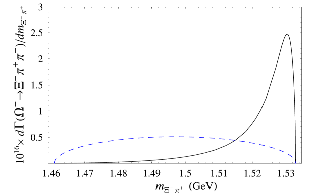
Figure 3: Distributions of $\Xi^{-}\pi^{+}$ invariant-mass in  $\Omega^{-}\to\Xi^{-}\pi^{+}\pi^{-}$  obtained from our leading-order amplitude (solid curve) and from the assumption of uniform-phase-space decay distribution (dashed curve), both normalized to yield  ${\cal B}(\Omega^{-}\to\Xi^{-}\pi^{+}\pi^{-})=3.6\times 10^{-4}$  .

III Calculation to next-to-leading order

At next-to-leading order, ${\cal O}(p)$, there are two types of contributions. The first type of contributions is that in which the weak transition occurs only between mesons. To compute these contributions, we need the leading-order, ${\cal O}(p^{2})$, strong and weak Lagrangians for mesons, which are given respectively by Gasser:1983yg ; Cronin:1967jq

$${\cal L}_{\rm s}^{\prime}\,\,=\,\,\mbox{$\frac{1}{4}$}f^{2}\left\langle\partial^{\mu}\Sigma^{\dagger}\,\partial_{\mu}\Sigma\right\rangle+\mbox{$\frac{1}{2}$}B_{0}f^{2}\left\langle M_{+}\right\rangle\,\,,$$ (11a)

$${\cal L}_{\rm w}^{\prime}\,\,=\,\,\gamma_{8}f^{2}\left\langle h\,\partial_{\mu}\Sigma\,\partial^{\mu}\Sigma^{\dagger}\right\rangle\,\,+\,\,{\rm H.c.}\,\,,$$ (11b)

where the parameter $\gamma_{8}$ is found from $\,K\to\pi\pi$  data to be

$$\gamma_{8}\,\,=\,\,-7.8\times 10^{-8}\,\,,$$ (12)

the sign following from various predictions g8 .

The contributions of the $\gamma_{8}$ term are interesting because the  $|\Delta S|=1$  weak transitions in the meson sector are larger than naive expectations. In particular, $\gamma_{8}$ is several times larger than its naturally expected value $\bigl{(}\sim$$1\times 10^{-8}\bigr{)}$ and therefore could make its contributions numerically comparable to the lower-order ones.

With weak vertices from the $\gamma_{8}$ term alone, plus strong vertices from ${\cal L}_{\rm s}$ and ${\cal L}_{\rm s}^{\prime}$, we derive the next-to-leading-order (NLO) diagrams displayed in Fig. 4. They provide the NLO contributions to the $A_{\pm}$ and $B_{\pm}$ form factors in Eq. (1), namely

$$A_{+}^{(1)}\,\,=\,\,\frac{-{\cal C}\,\gamma_{8}}{f^{2}}\,\,\frac{m_{\pi}^{2}-s_{+-}}{m_{K}^{2}-s_{+-}}\,\,,$$ (13a)

$$A_{-}^{(1)}\,\,=\,\,A_{+}^{(1)}\,\,,$$ (13b)

$$B_{+}^{(1)}\,\,=\,\,\frac{-\cal C\,H}{3f^{2}}\,\,\frac{\gamma_{8}\,m_{\pi}^{2}}{\bigl{(}m_{K}^{2}-m_{\pi}^{2}\bigr{)}\bigl{(}E_{\Xi}+E_{+}-\bar{m}_{\Xi^{*}}\bigr{)}}\,\,,$$ (13c)

$$B_{-}^{(1)} = \frac{-{\cal C}\,(D-F)}{f^{2}}\,\,\frac{\gamma_{8}\,m_{\pi}^{2}}{\bigl{(}m_{K}^{2}-m_{\pi}^{2}\bigr{)}\bigl{(}E_{\Xi}+E_{+}-m_{\Xi}\bigr{)}}$$ (13d)

$$+\,\,\frac{2\cal C\,H}{9f^{2}}\,\,\frac{\gamma_{8}\,m_{\pi}^{2}}{\bigl{(}m_{K}^{2}-m_{\pi}^{2}\bigr{)}\bigl{(}E_{\Xi}+E_{+}-\bar{m}_{\Xi^{*}}\bigr{)}}\,\,.$$

Figure 4: Diagrams contributing to  $\Omega^{-}\to\Xi^{-}\pi^{+}\pi^{-}$  at next-to-leading order in $\chi$PT. Each solid dot represents a strong vertex from ${\cal L}_{\rm s}$ in Eq. (4) or ${\cal L}_{\rm s}^{\prime}$ in Eq. (11a), and each square a weak vertex from ${\cal L}_{\rm w}^{\prime}$ in Eq. (11b).

There is another type of NLO contribution to the amplitudes. It is given by diagrams similar to those in Fig. 1 in which one of the vertices is from a NLO Lagrangian. Many of the parameters in NLO Lagrangians are not known, and so it is not possible at present to include their contributions in a detailed way. For example, the weak Lagrangian at ${\cal O}(p)$ that generates  $\Omega^{-}\Xi^{*}\pi$  and  $\Omega^{-}\Xi\pi$  vertices is, as discussed in Appendix A,

$$\tilde{\cal L}_{\rm w}^{\prime} = \frac{h_{\Omega\Xi^{*}\pi}}{f}\,v^{\alpha}\,\partial_{\alpha}\pi^{+}\,\bar{\Xi}^{*0}\cdot\Omega^{-}\,+\,\frac{\tilde{h}_{\Omega\Xi^{*}\pi}}{f}\,\partial_{\alpha}\pi^{+}\,\bar{\Xi}_{\mu}^{*0}\,2S_{v}^{\alpha}\,\Omega^{-\mu}$$ (14)

$$+\,\,\frac{h_{\Omega\Xi\pi}}{f}\,\partial^{\mu}\pi^{+}\,\bar{\Xi}^{0}\,\Omega_{\mu}^{-}\,\,+\,\,\cdots\,\,,$$

where only the relevant terms are displayed and $h_{\Omega\Xi^{*}\pi}$, $\tilde{h}_{\Omega\Xi^{*}\pi}$, and $h_{\Omega\Xi\pi}$ contain unknown parameters. The vertices occur in diagrams similar to the first one in Fig. 1 with intermediate $\Xi^{*}$ and $\Xi$, yielding the NLO contributions

$$\tilde{A}_{+}^{(1)}\,\,=\,\,\frac{-{\cal C}\,h_{\Omega\Xi^{*}\pi}\,E_{-}}{\sqrt{6}\,f^{2}\,\bigl{(}E_{\Xi}+E_{+}-\bar{m}_{\Xi^{*}}\bigr{)}}\,\,,$$ (15a)

$$\tilde{A}_{-}^{(1)}\,\,=\,\,0\,\,,$$ (15b)

$$\tilde{B}_{+}^{(1)}\,\,=\,\,\frac{-{\cal C}\,\tilde{h}_{\Omega\Xi^{*}\pi}}{\sqrt{6}\,f^{2}\,\bigl{(}E_{\Xi}+E_{+}-\bar{m}_{\Xi^{*}}\bigr{)}}\,\,,$$ (15c)

$$\tilde{B}_{-}^{(1)}\,\,=\,\,\frac{(D-F)\,h_{\Omega\Xi\pi}}{\sqrt{2}\,f^{2}\,\bigl{(}E_{\Xi}+E_{+}-m_{\Xi}\bigr{)}}\,+\,\frac{2{\cal C}\,\tilde{h}_{\Omega\Xi^{*}\pi}}{3\sqrt{6}\,f^{2}\,\bigl{(}E_{\Xi}+E_{+}-\bar{m}_{\Xi^{*}}\bigr{)}}\,\,.$$ (15d)

Numerically, we adopt the parametric variations

$$0\,\,\leq\,\,\bigl{|}h_{\Omega\Xi^{*}\pi}\bigr{|},\,\bigl{|}\tilde{h}_{\Omega\Xi^{*}\pi}\bigr{|},\,\bigl{|}h_{\Omega\Xi\pi}\bigr{|}\,\,\leq\,\,2\times 10^{-8}\,\,,$$ (16)

where the upper limit is the expectation from naive dimensional analysis.

As mentioned above, there are additional NLO contributions that are not included in our calculation because they depend on more unknown parameters. We can still estimate the uncertainty in our results arising from those terms by allowing the LO parameters to vary between their value as obtained from tree-level fits and their value as obtained from one-loop fits. For our numerics we will specifically consider parameter values obtained from fits at one-loop order, which are available in the literature Jenkins:1991ne ; Butler:1992pn ; Egolf:1998vj . We begin by noticing that our results in Eqs. (6), (13), and (15) show that $f$ is a common factor affecting the overall normalization only. Similarly, $\cal C$ is a common factor, except for the first term in Eq. (15d), which is numerically small. Consequently, we fix $f$ and $\cal C$ to their tree-level values, noting that the resulting decay rate scales with an overall factor  ${\cal C}^{2}/f^{4}$.  In addition, we keep $\gamma_{8}$ at its value in Eq. (12), as it is well determined. Thus, the ranges of the strong parameters we consider are

$$0.21\,\,\leq\,\,D-F\,\,\leq\,\,0.34\,\,,\hskip 20.00003pt-2.4\,\,\leq\,\,{\cal H}\,\,\leq\,\,-1.6\,\,.$$ (17)

On the other hand, since the range of the weak parameter $h_{C}$ from one-loop fits is large Egolf:1998vj ,  $-2\lesssim 10^{7}\,h_{C}\lesssim 4$,  we let it vary so as to reproduce the experimental decay rates.

In Fig. 5(a) we display the branching ratios calculated from the leading-order (LO) and NLO amplitudes above. The black (dark gray) band in the figure shows the effects of the parametric variations given in Eq. (17) on the branching ratio obtained from the LO amplitude alone (the LO amplitude and only the $\gamma_{8}$ terms in the NLO amplitude). The light-gray region results from the LO and NLO amplitudes considered above and varying the parameters according to Eqs. (16) and (17). The dotted lines in this figure bound the range  $3.3\leq 10^{4}\,{\cal B}(\Omega^{-}\to\Xi^{-}\pi^{+}\pi^{-})\leq 3.9$  implied by the preliminary HyperCP data. Evidently, this data can be reproduced in the three cases.

The corresponding $m_{\Xi^{-}\pi^{+}}$ distributions are plotted in Figs. 5(b) and (c) for  $h_{C}<0$  and  $h_{C}>0$,  respectively, with the variations of the other parameters for the different bands being the same as in Fig. 5(a). The $h_{C}$ ranges used in (b) and (c) are  $0.84<10^{8}\,|h_{C}|<0.92$  for the black bands,  $-1.05<10^{8}\,h_{C}<-0.90$  and  $0.55<10^{8}\,h_{C}<0.65$  for the dark-gray bands, and  $-1.8<10^{8}\,h_{C}<0$  and  $0<10^{8}\,h_{C}<1.4$  for the light-gray bands, all of which have been inferred from the corresponding bands in (a). The figures indicate that some softening of the $\Xi^{*}$ dominance in the spectrum is possible with the inclusion of higher-order contributions.

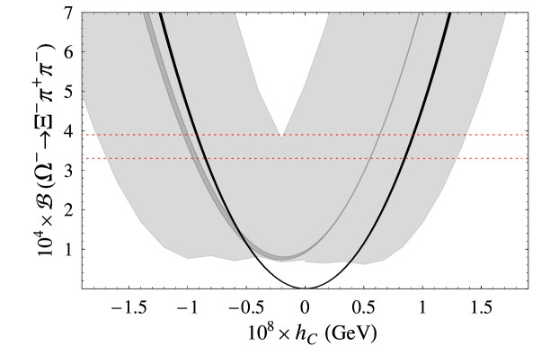
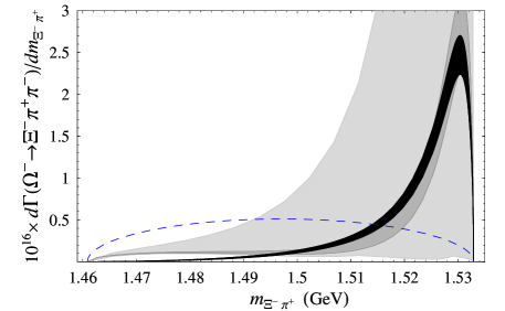
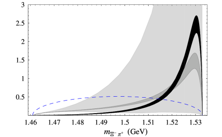
Figure 5: (a) Branching ratios for  $\Omega^{-}\to\Xi^{-}\pi^{+}\pi^{-}$  and (b,c) the corresponding distributions of $\Xi^{-}\pi^{+}$ invariant-mass. The black (dark gray) bands come from the LO amplitude only (the LO amplitude and the $\gamma_{8}$ terms in the NLO amplitude), and the light-gray bands result from the LO and NLO amplitudes we consider, as described in the text. The dotted lines in (a) bound the range implied by the preliminary HyperCP data. The dashed curves in (b) and (c) have been reproduced from Fig. 3.

IV Conclusions

We have evaluated the decay  $\Omega^{-}\to\Xi^{-}\pi^{+}\pi^{-}$  in heavy-baryon chiral perturbation theory. At leading order, we found a spectrum dominated by the $\Xi^{*}(1530)$, as had been suggested before. This shape is in conflict with the recent preliminary data from HyperCP. The total branching ratio is also in conflict with experiment for the central values of ${\cal C}$ and $h_{C}$, but it suffers from a large parametric uncertainty. This uncertainty, however, does not affect the shape of the $m_{\Xi^{-}\pi^{+}}$ invariant mass distribution.

A complete calculation at next-to-leading-order contains too many unknown parameters to be phenomenologically useful. We have investigated the effect of the NLO corrections in three different ways. First, we considered the diagrams in which the weak transition occurs in the meson sector. These corrections are induced by the low-energy constant $\gamma_{8}$ which is known from kaon decay. Second, we considered the NLO terms in the weak chiral Lagrangian which introduce three new effective constants. We studied the effect of these constants by varying their value between zero and the value suggested by naive dimensional analysis. Third and last, we varied the LO parameters in ranges that included their values as determined from tree-level and one-loop fits to other hyperon decay modes. The difference between the two kinds of fit is indicative of the size of NLO counterterms that we have not included explicitly. When all these factors are considered, we have found that it is possible to lower the branching ratio and soften the importance of the $\Xi^{*}$ in the $m_{\Xi^{-}\pi^{+}}$ distribution, as suggested by the data. Beyond this, we can only encourage the HyperCP collaboration to fit their data to our result, given in Eqs. (6), (13), and (15).

Appendix A Derivation of next-to-leading-order weak Lagrangian

The NLO weak Lagrangian generating the weak  $\Omega^{-}T\varphi$  vertices generally contains the Dirac structures  $\bar{T}^{\mu}\,v\cdot{\cal A}\,T_{\mu}$  and  $\bar{T}^{\mu}\,2S\cdot{\cal A}\,T_{\mu}$.  The only possible SU(3) building-blocks needed to construct it are therefore the tensors $\bar{T}_{abc}$, ${\cal A}_{de}$, and $T_{fgh}$. Employing standard techniques tdlee , we treat the combination  $\bar{T}_{abc}\,{\cal A}_{de}\,T_{fgh}$  as a tensor product  $\bigl{(}\overline{10}\otimes 8\bigr{)}\otimes 10$.  Thus we find four different operators that transform as octets, whose irreducible representations are

$$\begin{array}[]{c}\displaystyle\bigl{(}{\cal O}_{1}\bigr{)}_{ab}\,\,=\,\,\epsilon_{bmn}\,\bar{o}_{m,r}\,T_{anr}\,\,,\hskip 20.00003pt\bigl{(}{\cal O}_{2}\bigr{)}_{ab}\,\,=\,\,\bar{d}_{bmn}\,T_{amn}-\mbox{$\frac{1}{3}$}\,\delta_{ab}\,\bar{d}_{mno}\,T_{mno}\,\,,\vspace{2ex}\\ \displaystyle\bigl{(}{\cal O}_{3}\bigr{)}_{ab}\,\,=\,\,\epsilon_{bmn}\,\bar{\tau}_{am,op}\,T_{nop}\,\,,\hskip 20.00003pt\bigl{(}{\cal O}_{4}\bigr{)}_{ab}\,\,=\,\,\bar{\theta}_{a,bmno}\,T_{mno}\,\,,\end{array}$$ (20)

where

$$\bar{o}_{a,b}\,\,=\,\,\epsilon_{amn}\,\bar{T}_{bmo}\,{\cal A}_{on}\,\,,\hskip 30.00005pt\bar{d}_{abc}\,\,=\,\,\bar{T}_{abm}\,{\cal A}_{mc}+\bar{T}_{acm}\,{\cal A}_{mb}+\bar{T}_{bcm}\,{\cal A}_{ma}\;,$$ (21)

$$\bar{\tau}_{ab,cd} = \bar{T}_{cdm}\,\bigl{(}\epsilon_{amo}\,{\cal A}_{bo}+\epsilon_{bmo}\,{\cal A}_{ao}\bigr{)}$$ (22)

$$-\,\,\mbox{$\frac{1}{5}$}\bigl{(}\delta_{ac}\bar{T}_{dmn}\,\epsilon_{bmo}+\delta_{ad}\bar{T}_{cmn}\,\epsilon_{bmo}+\delta_{bc}\bar{T}_{dmn}\,\epsilon_{amo}+\delta_{bd}\bar{T}_{cmn}\,\epsilon_{amo}\bigr{)}\,{\cal A}_{no}\,\,,$$

$$\bar{\theta}_{a,bcde} = \bar{T}_{bcd}\,{\cal A}_{ae}+\bar{T}_{bce}\,{\cal A}_{ad}+\bar{T}_{bde}\,{\cal A}_{ac}+\bar{T}_{cde}\,{\cal A}_{ab}$$ (23)

$$-\,\,\mbox{$\frac{1}{6}$}\,\delta_{ab}\bigl{(}\bar{T}_{cdm}\,{\cal A}_{me}+\bar{T}_{cem}\,{\cal A}_{md}+\bar{T}_{dem}\,{\cal A}_{mc}\bigr{)}$$

$$-\,\,\mbox{$\frac{1}{6}$}\,\delta_{ac}\bigl{(}\bar{T}_{bdm}\,{\cal A}_{me}+\bar{T}_{bem}\,{\cal A}_{md}+\bar{T}_{dem}\,{\cal A}_{mb}\bigr{)}$$

$$-\,\,\mbox{$\frac{1}{6}$}\,\delta_{ad}\bigl{(}\bar{T}_{bcm}\,{\cal A}_{me}+\bar{T}_{cem}\,{\cal A}_{mb}+\bar{T}_{bem}\,{\cal A}_{mc}\bigr{)}$$

$$-\,\,\mbox{$\frac{1}{6}$}\,\delta_{ae}\bigl{(}\bar{T}_{bcm}\,{\cal A}_{md}+\bar{T}_{cdm}\,{\cal A}_{mb}+\bar{T}_{bdm}\,{\cal A}_{mc}\bigr{)}\;.$$

The tensors $({\cal O}_{1,2,3,4})_{ab}$ and $\bar{o}_{ab}$ are all traceless, $\bar{d}_{abc}$ is fully symmetric in its indices, $\bar{\tau}_{ab,cd}$ satisfies the symmetry relation  $\bar{\tau}_{ab,cd}=\bar{\tau}_{ba,cd}=\bar{\tau}_{ab,dc}=\bar{\tau}_{ba,dc}$  and tracelessness condition  $\bar{\tau}_{ab,cb}=0$,  and $\bar{\theta}_{a,bcde}$ is symmetric in its $bcde$ indices and satisfies  $\bar{\theta}_{a,abcd}=0$.

The only possible building blocks needed to construct the NLO weak Lagrangian generating the weak  $\Omega^{-}B\varphi$  vertices are the tensors $\;\bar{B}_{ab}$, ${\cal A}_{cd}$, and $T_{def}$. Treating the combination  $\bar{B}_{ab}\,{\cal A}_{cd}\,T_{def}$  as a tensor product  $(8\otimes 8)\otimes 10$,  we find four different operators that transform as octets, whose irreducible representations are

$$\begin{array}[]{c}\displaystyle\bigl{(}{\cal O}_{1}^{\prime}\bigr{)}_{ab}\,\,=\,\,\epsilon_{bmn}\,\bar{\cal D}_{mo}\,T_{ano}\,\,,\hskip 20.00003pt\bigl{(}{\cal O}_{2}^{\prime}\bigr{)}_{ab}\,\,=\,\,\epsilon_{bmn}\,\bar{\cal F}_{mo}\,T_{ano}\,\,,\vspace{2ex}\\ \displaystyle\bigl{(}{\cal O}_{3}^{\prime}\bigr{)}_{ab}\,\,=\,\,\bar{t}_{bmn}\,T_{amn}-\mbox{$\frac{1}{3}$}\,\delta_{ab}\,\bar{t}_{mno}\,T_{mno}\,\,,\hskip 20.00003pt\bigl{(}{\cal O}_{4}^{\prime}\bigr{)}_{ab}\,\,=\,\,\epsilon_{bmn}\,\bar{\cal T}_{am,op}\,T_{nop}\,\,,\end{array}$$ (26)

where

$$\bar{\cal D}_{ab}\;=\;\bigl{\{}\bar{B},{\cal A}\bigr{\}}_{ab}-\mbox{$\frac{2}{3}$}\,\bigl{\langle}\bar{B}{\cal A}\bigr{\rangle}\,\delta_{ab}\,\,,\hskip 30.00005pt\bar{\cal F}_{ab}\;=\;\bigl{[}\bar{B},{\cal A}\bigr{]}_{ab}\;,$$ (27)

$$\bar{t}_{abc} = \epsilon_{amn}\left(\bar{B}_{mb}{\cal A}_{nc}+\bar{B}_{mc}{\cal A}_{nb}\right)+\epsilon_{bmn}\left(\bar{B}_{mc}{\cal A}_{na}+\bar{B}_{ma}{\cal A}_{nc}\right)$$ (28)

$$+\,\,\epsilon_{cmn}\left(\bar{B}_{ma}{\cal A}_{nb}+\bar{B}_{mb}{\cal A}_{na}\right)\;,$$

$$\bar{\cal T}_{ab,cd} = \bar{B}_{ac}{\cal A}_{bd}+\bar{B}_{ad}{\cal A}_{bc}+\bar{B}_{bc}{\cal A}_{ad}+\bar{B}_{bd}{\cal A}_{ac}$$ (29)

$$-\,\,\mbox{$\frac{1}{5}$}\left(\delta_{ac}\bar{\cal D}_{bd}+\delta_{ad}\bar{\cal D}_{bc}+\delta_{bc}\bar{\cal D}_{ad}+\delta_{bd}\bar{\cal D}_{ac}\right)\,-\,\mbox{$\frac{1}{6}$}\left(\delta_{ac}\delta_{bd}+\delta_{ad}\delta_{bc}\right)\bigl{\langle}\bar{B}{\cal A}\bigr{\rangle}\,\,.$$

The tensors $({\cal O}_{1,2,3,4}^{\prime})_{ab}$, $\bar{\cal D}_{ab}$, and $\bar{\cal F}_{ab}$ are all traceless, $\bar{t}_{abc}$ is fully symmetric in its indices, and $\bar{\cal T}_{ab,cd}$ satisfy the symmetry relation  $\bar{\cal T}_{ab,cd}=\bar{\cal T}_{ba,cd}=\bar{\cal T}_{ab,dc}=\bar{\cal T}_{ba,dc}$  and tracelessness condition  $\bar{\cal T}_{ab,cb}=0$.

The resulting NLO weak Lagrangian that contributes to  $\Omega^{-}\to\Xi^{*}\pi,\Xi\pi$  and transforms as $(8_{\rm L},1_{\rm R})$ is then

$$\tilde{\cal L}_{\rm w}^{\prime} = \left\langle\xi^{\dagger}h\xi\left(h_{1}\,{\cal O}_{1}+h_{2}\,{\cal O}_{2}+h_{3}\,{\cal O}_{3}+h_{4}\,{\cal O}_{4}\right)\right\rangle$$ (30)

$$+\,\,\left\langle\xi^{\dagger}h\xi\left(\tilde{h}_{1}\,\tilde{\cal O}_{1}+\tilde{h}_{2}\,\tilde{\cal O}_{2}+\tilde{h}_{3}\,\tilde{\cal O}_{3}+\tilde{h}_{4}\,\tilde{\cal O}_{4}\right)\right\rangle$$

$$+\,\,\left\langle\xi^{\dagger}h\xi\left(h_{1}^{\prime}\,{\cal O}_{1}^{\prime}+h_{2}^{\prime}\,{\cal O}_{2}^{\prime}+h_{3}^{\prime}\,{\cal O}_{3}^{\prime}+h_{4}^{\prime}\,{\cal O}_{4}^{\prime}\right)\right\rangle\,\,,$$

where ${\cal O}_{i}$ and $\tilde{\cal O}_{i}$ contain the Dirac structures  $\bar{T}^{\mu}\,v\cdot{\cal A}\,T_{\mu}$  and  $\bar{T}^{\mu}\,2S\cdot{\cal A}\,T_{\mu}$, respectively, and $h_{i}$, $\tilde{h}_{i}$, and $h_{i}^{\prime}$ and are free parameters. Expanding the Lagrangian yields

$$\tilde{\cal L}_{\rm w}^{\prime} = \frac{h_{\Omega\Xi^{*}\pi}}{f}\,v^{\alpha}\,\partial_{\alpha}\pi^{+}\,\bar{\Xi}^{*0}\cdot\Omega^{-}\,+\,\frac{\tilde{h}_{\Omega\Xi^{*}\pi}}{f}\,\partial_{\alpha}\pi^{+}\,\bar{\Xi}_{\mu}^{*0}\,2S_{v}^{\alpha}\,\Omega^{-\mu}$$ (31)

$$+\,\,\frac{h_{\Omega\Xi\pi}}{f}\,\partial^{\mu}\pi^{+}\,\bar{\Xi}^{0}\,\Omega_{\mu}^{-}\,\,+\,\,\cdots\,\,,$$

where

$$\begin{array}[]{c}\displaystyle\stackrel{{\scriptstyle\scriptscriptstyle(\sim)}}{{h}}_{\Omega\Xi^{*}\pi}\,\,=\,\,\frac{\stackrel{{\scriptstyle\scriptscriptstyle(\sim)}}{{h}}_{1}}{\sqrt{6}}+\frac{\stackrel{{\scriptstyle\scriptscriptstyle(\sim)}}{{h}}_{2}}{\sqrt{6}}-\frac{7\,\stackrel{{\scriptstyle\scriptscriptstyle(\sim)}}{{h}}_{3}}{5\sqrt{6}}-\frac{\stackrel{{\scriptstyle\scriptscriptstyle(\sim)}}{{h}}_{4}}{2\sqrt{6}}\,\,,\vspace{2ex}\\ \displaystyle h_{\Omega\Xi\pi}\,\,=\,\,\frac{-h_{1}^{\prime}}{\sqrt{2}}+\frac{h_{2}^{\prime}}{\sqrt{2}}-\sqrt{2}\,h_{3}^{\prime}+\frac{\sqrt{2}\,h_{4}^{\prime}}{5}\,\,.\end{array}$$ (34)

References

(1)
D.N. Goswami and J. Schechter,
Phys. Rev. D 1, 290 (1970)
[Erratum-ibid. D 4, 3526 (1971)].
(2)
J. Finjord and M.K. Gaillard,
Phys. Rev. D 22, 778 (1980).
(3)
W.M. Yao et al. [Particle Data Group],
J. Phys. G 33, 1 (2006).
(4)
M. Bourquin et al.,
Nucl. Phys. B 241, 1 (1984).
(5)
N. Solomey,
Nucl. Phys. Proc. Suppl. 115, 54 (2003)
[arXiv:hep-ex/0208026];
O. Kamaev [HyperCP Collaboration],
AIP Conf. Proc. 842, 452 (2006);
Talk given at the Joint Meeting of Pacific Region Particle Physics Communities,
29 October – 3 November 2006, Honolulu, Hawaii.
(6)
J. Gasser and H. Leutwyler,
Annals Phys. 158, 142 (1984).
(7)
J. Bijnens, H. Sonoda, and M.B. Wise,
Nucl. Phys. B 261, 185 (1985).
(8)
E. Jenkins and A.V. Manohar, Phys. Lett. B 255, 558 (1991);
ibid.259, 353 (1991);
E. Jenkins, Nucl. Phys. B368, 190 (1992);
in Effective Field Theories of the Standard Model, edited by
U.-G. Meissner (World Scientific, Singapore, 1992).
(9)
E. Jenkins,
Nucl. Phys. B 375, 561 (1992).
(10)
J. A. Cronin,
Phys. Rev. 161, 1483 (1967).
(11)
R.S. Chivukula and A.V. Manohar,
Phys. Lett. B 207, 86 (1988)
[Erratum-ibid. B 217, 568 (1989)];
J.F. Gunion, H.E. Haber, G.L. Kane, and S. Dawson,
The Higgs Hunter’s Guide (The Perseus Books Group, New York, 2000).
(12)
M.N. Butler, M.J. Savage, and R.P. Springer,
Nucl. Phys. B 399, 69 (1993)
[arXiv:hep-ph/9211247].
(13)
D.A. Egolf, I.V. Melnikov, and R.P. Springer,
Phys. Lett. B 451, 267 (1999)
[arXiv:hep-ph/9809228];
R.P. Springer,
ibid. 461, 167 (1999);
A. Abd El-Hady and J. Tandean,
Phys. Rev. D 61, 114014 (2000)
[arXiv:hep-ph/9908498].
(14)
See, e.g., T.D. Lee, Particle Physics and Introduction to Field Theory
(Harwood Academic, New York, 1981).