Boson decay and the dynamical structure factor for the $XXZ$ chain at finite magnetic field

Abstract

We study the longitudinal dynamical structure factor $S^{zz}(q,\omega)$ for the anisotropic spin-$1/2$ ($XXZ$) chain at finite magnetic field using bosonization. The leading irrelevant operators in the effective bosonic model stemming from band curvature describe boson decay processes and lead to a high-frequency tail and a finite width $\gamma_{q}$ of the on-shell peak for $S^{zz}(q,\omega)$. We use the Bethe ansatz to show that $\gamma_{q}\sim q^{2}$ for $q\ll 1$ and to calculate the amplitudes of the leading irrelevant operators in the effective field theory.

, , , , , ,

1 Introduction

The Hamiltonian of the $XXZ$ spin chain is given by

$$H=J\sum_{j=1}^{N}\left[S_{j}^{x}S_{j+1}^{x}+S_{j}^{y}S_{j+1}^{y}+\Delta S_{j}^{z}S_{j+1}^{z}-hS_{j}^{z}\right]\;.$$ (1)

Here $J$ is the exchange coupling, $\Delta$ the anisotropy, $h$ a magnetic field and $N$ the number of sites. The isotropic model ($\Delta=1$) has direct applications to compounds like Sr₂CuO₃ where copper-oxygen chains form along one crystal axis and the coupling between these chains is very weak making them effectively one dimensional. Furthermore, the system (1) can be mapped exactly onto interacting spinless fermions using the Jordan-Wigner transformation. In this language $\Delta$ parametrizes a nearest-neighbor density-density interaction and $h$ becomes the chemical potential. The fermionic version of (1) is often used as a simple model for quantum wires [1].

The $XXZ$ model is exactly solvable by means of Bethe Ansatz (BA). However, the calculation of correlation function by BA is a difficult task and only limited results have been obtained so far. On the other hand, it is known that the low-energy effective theory for the Hamiltonian (1) is just a free boson model. This so called Luttinger liquid Hamiltonian $H_{LL}$ is obtained by linearizing the dispersion around the two Fermi points, going to the continuum limit and reexpressing the right- and left-moving fermions by bosons. Ignoring irrelevant operators this leads to

$$H_{LL}=\frac{v}{2}\int dx\left[\Pi^{2}+\left(\partial_{x}\phi\right)^{2}\right]\,.$$ (2)

Here, $\phi(x)$ is a bosonic field and $\Pi(x)$ its conjugated momentum satisfying $[\phi(x),\Pi(y)]=i\delta(x-y)$. As a consequence of the linearized dispersion the Hamiltonian (2) is Lorentz invariant and a boson with momentum $|q|$ always carries energy $\omega=v|q|$. In the following we will investigate corrections to (2) due to band curvature and consequences for the lineshape of the dynamical structure factor.

2 The dynamical structure factor

The longitudinal dynamical structure factor is defined by

$$S^{zz}\left(q,\omega\right) = \frac{1}{N}\sum_{j,j^{\prime}=1}^{N}e^{-iq\left(j-j^{\prime}\right)}\int_{-\infty}^{+\infty}dt\,e^{i\omega t}\left\langle S_{j}^{z}\left(t\right)S_{j^{\prime}}^{z}\left(0\right)\right\rangle$$ (3)

$$= \frac{2\pi}{N}\sum_{\alpha}\left|\left\langle 0\left|S_{q}^{z}\right|\alpha\right\rangle\right|^{2}\delta\left(\omega-E_{\alpha}\right)\;.$$

Here $S_{q}^{z}=\sum_{j}S_{j}^{z}e^{-iqj}$ and $\left|\alpha\right\rangle$ is an eigenstate with energy $E_{\alpha}$ above the ground state energy. For a finite system, $S^{zz}\left(q,\omega\right)$ at fixed $q$ is a sum of $\delta$-peaks at the energies of the eigenstates. In the thermodynamic limit $N\rightarrow\infty$, the spectrum is continuous and $S^{zz}\left(q,\omega\right)$ becomes a smooth function of $\omega$ and $q$. Due to Lorentz invariance $S^{zz}\left(q,\omega\right)=K\left|q\right|\delta\left(\omega-v\left|q\right|\right)$ for the Luttinger model (2).

For $h\neq 0$ particle-hole symmetry is broken and the leading irrelevant operators allowed by symmetry are the dimension-three operators $\sim(\partial_{x}\phi_{R,L})^{3}$. More precisely, we consider the following correction to (2)

$$\delta H = \int dx\,\bigg{\{}\eta_{-}\left[\left(\partial_{x}\phi_{L}\right)^{3}-\left(\partial_{x}\phi_{R}\right)^{3}\right]$$

$$+ \eta_{+}\left[\left(\partial_{x}\phi_{L}\right)^{2}\partial_{x}\phi_{R}-\left(\partial_{x}\phi_{R}\right)^{2}\partial_{x}\phi_{L}\right]\bigg{\}}\;,$$

where $\phi_{R,L}$ are the right- and left-moving components of the bosonic field with $\phi=(\phi_{L}-\phi_{R})/\sqrt{2}$. This correction is the bosonized form of the leading band curvature term $\omega(q)=\pm vq+q^{2}/(2m)+\cdots$. Note, that (2) corresponds to interaction vertices allowing a boson to decay into two bosons. The $\eta_{+}$-interaction allows for intermediate states with one right- and one left-moving boson, which together can carry small momentum but high energy $\omega\gg v\left|q\right|$ thus giving rise to a high-energy tail in $S^{zz}(q,\omega)$. The $\eta_{-}$-interaction, on the other hand, will influence the on-shell part $\omega\sim vq$. If $\gamma_{q}\ll\omega-v|q|\ll J$, where $\gamma_{q}$ is the width if the on-shell peak, then the terms in (2) can be treated in perturbation theory and we find a high-frequency tail [2]

$$\delta S^{zz}_{\eta_{+}}\left(q,\omega\right)=\frac{K\eta_{+}^{2}q^{4}}{v\pi}\,\frac{\theta\left(\omega-v\left|q\right|\right)}{\omega^{2}-v^{2}q^{2}}.$$ (5)

The parameters $\eta_{\pm}$ can be related to the change in the velocity $v$ and the Luttinger parameter $K$ when varying $h$ and we find $J\eta_{-}(h_{0})=\sqrt{2\pi/K}v^{2}(a+b/2)/6$ and $J\eta_{+}(h_{0})=\sqrt{2\pi/K}v^{2}b/4$ where $a=v^{-1}\partial v/\partial h|_{h=h_{0}}$ and $b=K^{-1}\partial K/\partial h|_{h=h_{0}}$ [2]. Due to the integrability of the model it is possible to obtain $v(h)$, $K(h)$ for all anisotropies and fields by BA so that (5) does not contain any free parameters. In Fig. 1 this analytical result is compared to a BA calculation for a chain with $N=200$ sites.

Figure 1: Analytical result for the high-frequency tail (5) (black solid line) compared to a BA calculation for a chain with $N=200$ (red dots). Here $\Delta=0.25$ and the magnetization $\langle s^{z}\rangle=-0.1$.

Perturbation theory in $\eta_{-}$, on the other hand, produces terms which become increasingly singular at $\omega\sim vq$. Therefore the whole series has to be summed up to produce a finite result [3]. Here we only present BA results for the form factors $F(q,\omega)\equiv\langle 0|S^{z}_{q}|\alpha\rangle$ (see (3)) for $\omega\sim vq$ in Fig. 2.

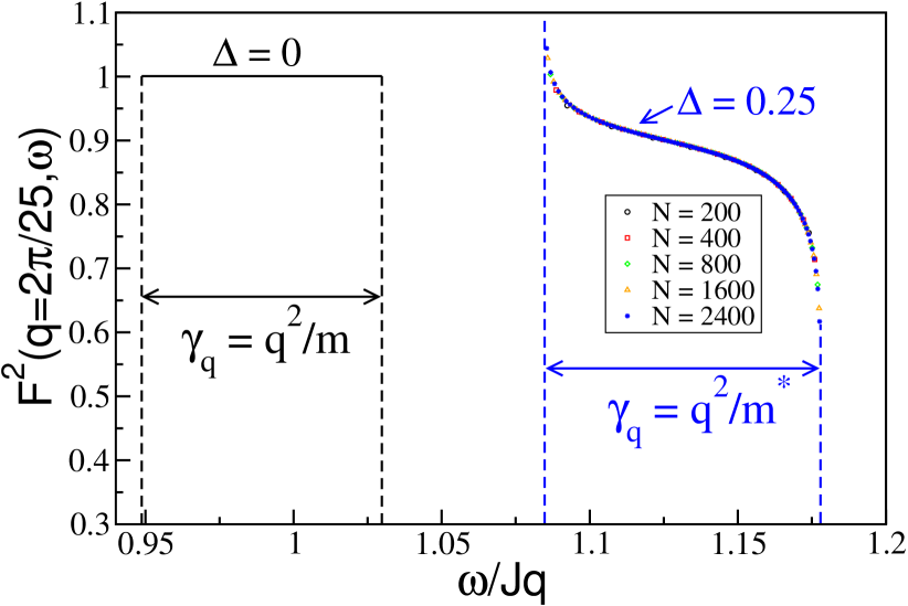
Figure 2: Exact solution for $F(q,\omega)$ at the free fermion point $\Delta=0$ compared to numerical BA data at $\Delta=0.25$ for different finite size systems with $\langle s^{z}\rangle=-0.1$ in both cases. The effective mass in the free fermion case is given by $m=(J\cos k_{F})^{-1}$ where $k_{F}$ is the Fermi momentum. For small finite $\Delta$ the effective mass can be obtained by BA and is given by $m^{*}=m/(1+2\Delta\sin k_{F}/\pi)$ [2].

Note that the width $\gamma_{q}$ of the on-shell peak for finite $\Delta$ is $\sim q^{2}$ as in the free fermion case ($\Delta=0$) but the effective mass is renormalized. For finite $\Delta\ll 1$, Pustilnik et al. [4] have shown that $S^{zz}(q,\omega)$ exhibits power laws at the upper and lower threshold of the on-shell peak with exponents depending on $\Delta$ and $q$. Their results are consistent with our numerical data shown in Fig. 2.

3 Acknowledgement

This research was supported by CNPq through Grant No. 200612/2004-2 (R.G.P), the DFG (J.S.), FOM (J.-S.C.), CNRS and the EUCLID network (J.M.M.), the NSF under DMR 0311843 (S.R.W.), and NSERC (J.S., I.A.) and the CIAR (I.A.).

References

- [1] M. Pustilnik, E. G. Mishenko, L. I. Glazman, and A. V. Andreev, Phys. Rev. Lett. 91 (2003) 126805.
- [2] R. G. Pereira, J. Sirker, J.-S. Caux, R. Hagemans, J. M. Maillet, S. R. White, and I. Affleck, Phys. Rev. Lett. 96 (2006) 257202.
- [3] R. G. Pereira, J. Sirker, J.-S. Caux, R. Hagemans, J. M. Maillet, S. R. White, and I. Affleck, in preparation.
- [4] M. Pustilnik, M. Khodas, A. Kamenev, and L. I. Glazman, Phys. Rev. Lett. 96 (2006) 196405.