Cold Plasma Dispersion Relations in the Vicinity of a Schwarzschild Black Hole Horizon

Abstract

We apply the ADM 3+1 formalism to derive the general relativistic magnetohydrodynamic equations for cold plasma in spatially flat Schwarzschild metric. Respective perturbed equations are linearized for non-magnetized and magnetized plasmas both in non-rotating and rotating backgrounds. These are then Fourier analyzed and the corresponding dispersion relations are obtained. These relations are discussed for the existence of waves with positive angular frequency in the region near the horizon. Our results support the fact that no information can be extracted from the Schwarzschild black hole. It is concluded that negative phase velocity propagates in the rotating background whether the black hole is rotating or non-rotating.

Keywords : 3+1 formalism, perturbations, dispersion relations.

1 Introduction

General Relativity (GR) serves both as a theory of space and time as well as a theory of gravitation. This theory has tremendous philosophical implications and has given rise to exotic new physical concepts like black holes and dark matter. All the predictions and applications by different scientists make the theory a spectacularly successful one. The theory of GR is not complete unless it includes the hard reality of experiments and of astronomical observations. To explain the phenomena observed by astronomers in physical terms we have astrophysical relativity. This serves as a tool to gauge the properties of large scale structures for which gravitation plays a significant role.

It is believed that the compact objects have strong gravitational fields near their surfaces [1]. The study of general relativistic effects on electromagnetic processes which take place in the vicinity of compact objects is of theoretical interest in its own right. However, it is also important to interpret and understand the still puzzling signals we receive from these astronomical objects, including neutron stars and black holes. All the massive stars, neutron stars and black holes carry energy flux. Due to this flux, a relatively large magnetic field is produced. In order to understand the phenomena of the compact objects and many more like these, we have a developed theory of magnetized plasma called theory of magnetohydrodynamics (MHD). To study the magnetosphere of massive black holes, the strength of gravity demands the theory of general relativistic magnetohydrodynamics (GRMHD). GRMHD equations help us to study stationary configurations and dynamic evolution of conducting fluid in a magnetosphere. These equations (Maxwell’s equations, Ohm’s law, mass, momentum and energy conservation equations) are required to investigate various aspects of the interaction of relativistic gravity with plasma’s magnetic field. The successful study of plasmas in the black hole environment is important because a successful study of waves will be of great value in aiding the observational identification of black hole candidates. It is well-known [2-4] that an isolated black hole cannot have an electromagnetic field unless it is endowed with a net electric charge. Since a collapsed object can have a very strong effect on an electromagnetic field, it is of interest to determine this effect when a black hole is placed in an external electromagnetic field using GRMHD equations.

The 3+1 formalism (also called ADM formalism) was originally developed to study the quantization of gravitational field by Arnowitt et al. [5]. Tarfulea [6] worked on numerical solutions of Einstein field equations by applying constraint preserving boundary conditions. Thorne and Macdonald [7,8] extended the formulation to electromagnetic fields. Thorne et al. [9] described its further applications for the black hole theory. The black hole theory was considered by Holcomb and Tajima [10], Holcomb [11] and Dettmann et al. [12] to investigate some properties of wave propagation in Friedmann universe. Khanna [13] derived the MHD equations describing the two component plasma theory of Kerr black hole in 3+1 split. Antón et al. [14] used 3+1 formalism to investigate various test simulations and discussed magneto-rotational instability of accretion disks. Anile [15] worked on propagation and stability of relativistic shocks and relativistic simple waves in magneto-fluids. He also linearized the electromagnetic wave theory in cold relativistic plasma. Komissarov [16] discussed Blendford-Znajec monopole solution using 3+1 formalism in black hole electrodynamics. In another paper [17], he formulated and solved time dependent, force free, degenerate electrodynamics as a hyperbolic system of conservations laws for pulsars. He also discussed the waves mode and one dimensional numerical scheme based on linear and exact Riemann solvers. Zhang [18] formulated the black hole theory for stationary symmetric GRMHD using $3+1$ formalism. The same author [19] applied this formulation to the linearized waves propagating in two dimensions using perfect GRMHD fluid for the cold plasma state in the vicinity of Kerr black hole magnetosphere. He investigated the behavior of perturbations in graphic form which described the response of the magnetosphere to oscillatory driving forces near the plasma-injection plane. Tsikarishvili et al. [20] considered 3+1 general relativistic hydrodynamical equations describing strongly magnetized collisionless plasma with an anisotropic pressure and obtained the equations of state in ultra-relativistic limit. In his recent paper, Mofiz [21] discussed gravitational waves in magnetized plasmas.

The formalism for gravitational perturbations away from a Scwarzschild background was developed by Regge and Wheeler [22]. It was extended by Zerilli [23] who proved that the perturbations corresponding to a change in mass, the angular momentum and charge, of the Schwarzschild black hole are well-behaved. The decay of non well-behaved perturbations was investigated by Price [24]. The quasi-static electric problem was solved by Hanni and Ruffini [25] who showed that the lines of force diverge at the horizon for the observer at infinity. Wald [26] derived the solution for electromagnetic field occurring when a stationary axisymmetric black hole is placed in a uniform magnetic field aligned along the symmetry axis of black hole. A linearized treatment of plasma waves for special relativistic formulation of Schwarzschild black holes was developed by Sakai and Kawata [27]. This treatment was extended to waves in general relativistic two component plasma in 3+1 ADM formalism, propagating in radial direction by Buzzi et al. [28]. They investigated the one dimensional radial propagation of transverse and longitudinal waves close to the Schwarzschild horizon.

This paper is devoted to study the dynamical magnetosphere of the Schwarzschild black hole. The model spacetime is the Schwarzschild metric in Rindler coordinates which preserves the key features of the Schwarzschild geometry. This investigation supports the well-known fact that the information from the black hole cannot be extracted. We apply 3+1 form of the GRMHD equations to this spacetime by using the cold plasma state. Afterwards, we linearize the equations to study perturbations of the magnetosphere. These equations are then Fourier analyzed to get the sets of ordinary differential equations which are comparatively easier to handle than the original GRMHD partial differential equations. The determinant of these equations are solved [29] to get dispersion relations. Since the determinant of the coefficients of the Fourier analyzed equations cannot be solved analytically, we solve it with the help of software Mathematica for special cases and wave numbers are obtained in terms of angular frequency and lapse function. We use wave number to calculate phase and group velocities, refractive index and change in refractive index w.r.t. angular frequency. The graphs of each of these quantities are given and discussed.

The paper has been organized as follows. In the next section, we shall review the general results for the 3+1 formalism. The GRMHD equations in the Schwarzschild black hole magnetosphere for the cold plasma are also given. In section $3$, we restrict the problem only to the non-rotating background. Section $4$ is devoted to the rotating non-magnetized plasma and section $5$ is furnished with the dispersion relations for the rotating magnetized plasma. In the last section, we shall summarize and discuss the results.

2 3+1 Spacetime Modelling

In the $3+1$ formalism, the line element of the spacetime can be written as [19]

$$ds^{2}=-\alpha^{2}dt^{2}+\gamma_{ij}(dx^{i}+\beta^{i}dt)(dx^{j}+\beta^{j}dt),$$ ( 2. 1)

where $\alpha$ (lapse function), $\beta^{i}$ (shift vector) and $\gamma_{ij}$ (spatial metric) are functions of the coordinates $t,~{}x^{i}$. A natural observer, associated with this spacetime called fiducial observer (FIDO), has four velocity n perpendicular to the hypersurfaces of constant time $t$ and is given by

$$\bf{n}=\frac{1}{\alpha}(\frac{\partial}{\partial t}-\beta^{i}\frac{\partial}{\partial x^{i}}).$$ ( 2. 2)

Throughout the paper, geometrized units with $G=c=1$ will be used. Vectors and tensors living in four-dimensional spacetime will be denoted by boldface italic letters such as FIDO’s four-velocity n. The three-dimensional tensors are distinguished from vectors by a dyad over the letter, such as three-dimensional metric $\overleftrightarrow{\gamma}$. All vector analysis notations such as gradient, curl and vector product will be those of the three dimensional absolute space with three metric $\overleftrightarrow{\gamma}$. The determinant of three metric is denoted as $g$: $g\equiv det|\gamma_{ij}|.$ Latin letters $i,j,k,...$ represent indices in absolute space and run from 1 to 3.

The Schwarzschild line element in Rindler coordinates [9]

$$ds^{2}=-\alpha^{2}(z)dt^{2}+dx^{2}+dy^{2}+dz^{2}$$ ( 2. 3)

is the best approximation of this spacetime in Cartesian coordinates. Since the Schwarzschild black hole is non-rotating, hence the shift vector $\beta=0$. This model is an analogue of the Schwarzschild spacetime with $z$, $x$ and $y$ as radial $r$, axial $\phi$ and poloidal $\theta$ directions respectively. $\alpha$ is the lapse function which depends on $r$ in the Shwarzschild metric, whereas it depends on $z$ in this analogue. In Rindler coordinates, $\alpha=\frac{z}{2r_{H}}$, where $r_{H}$ is the radius of the Schwarzschild black hole. This function vanishes at the horizon which we can place at $z=0$ and it increases monotonically as $z$ increases from $0$ to $\infty.$ The associated FIDO’s four-velocity vector reduces to $\textbf{n}=\frac{1}{\alpha}\frac{\partial}{\partial t}$. The constant time surfaces have spatial geometry $ds^{2}=dx^{2}+dy^{2}+dz^{2}$ which gives a good approximation to the Schwarzschild geometry near the horizon.

2.1 The 3+1 Split: Laws of Physics

The real power of 3+1 viewpoint lies in its strong similarity to a physicists with non-general relativistic experience. The 3+1 laws of electrodynamics are formulated with an eye towards emphasizing this similarity. However, there are real unavoidable and crucial new features of these familiar laws that enter electrodynamics in the vicinity of a black hole. The most important of these is the issue of two times, the universal time $t$ and the FIDO’s time $\tau$. Both times are related to each other by $\alpha\equiv\frac{d\tau}{dt}$. For the Schwarzschild black hole, the Maxwell equations in 3+1 formalism take the form [9]

$$\nabla.\textbf{B} = 0,$$ ( 2. 4)

$$\frac{\partial\textbf{B}}{\partial t} = -\nabla\times(\alpha\textbf{E}),$$ ( 2. 5)

$$\nabla.\textbf{E} = 4\pi\rho_{e},$$ ( 2. 6)

$$\frac{\partial\textbf{E}}{\partial t} = \nabla\times(\alpha\textbf{B})-4\pi\alpha\textbf{j},$$ ( 2. 7)

where B and E are the FIDO measured magnetic and electric fields, j and $\rho_{e}$ are electric current and electric charge density respectively. Under the perfect MHD condition, i.e.,

$$\textbf{E}+\textbf{V}\times\textbf{B}=0,$$ ( 2. 8)

where V is the velocity of the fluid measured by the FIDO, there can be no electric field in fluid’s rest frame. For perfect MHD, the equations of evolution of magnetic field [18] become

$$\frac{D\textbf{B}}{D\tau}+\frac{1}{\alpha}(\textbf{B}.\nabla)(\beta-\alpha\textbf{V})+\left\{\theta+\frac{1}{\alpha}\nabla.(\alpha\textbf{V})\right\}\textbf{B}=0,$$ ( 2. 9)

where

$$\frac{D}{D\tau}\equiv\frac{d}{d\tau}+\textbf{V}.\nabla=\frac{1}{\alpha}\left\{\frac{\partial}{\partial t}+(\alpha\textbf{V}-\beta).\nabla\right\}.$$

The expansion rate of FIDO’s four-velocity is

$$\theta=\frac{1}{\alpha}(\frac{\dot{g}}{2g}-\nabla.\beta).$$

Here dot indicates partial derivative with respect to time $t$. The FIDO’s measured rate of change of any three dimensional vector in absolute space (orthogonal to n) is

$$\frac{d}{d\tau}\equiv\frac{1}{\alpha}(\frac{\partial}{\partial t}-\beta.\nabla).$$

Local conservation law of rest-mass according to FIDO is given by [18]

$$\frac{D\rho_{0}}{D\tau}+\rho_{0}\gamma^{2}\textbf{V}.\frac{D\textbf{V}}{D\tau}+\frac{\rho_{0}}{\alpha}\left\{\frac{\dot{g}}{2g}+\nabla.(\alpha\textbf{V}-\beta)\right\}=0,$$

or

$$\frac{D\rho_{0}}{D\tau}+\rho_{0}\gamma^{2}\textbf{V}.\frac{D\textbf{V}}{D\tau}+\rho_{0}\left\{\theta+\frac{1}{\alpha}\nabla.(\alpha\textbf{V})\right\}=0$$ ( 2. 10)

with $\rho_{0}$ as the rest mass density. FIDO measured law of force balance equation can be written as

$$\left\{\left(\rho_{0}\gamma^{2}\mu+\frac{\textbf{B}^{2}}{4\pi}\right)\gamma_{ij}+\rho_{0}\gamma^{4}\mu V_{i}V_{j}-\frac{1}{4\pi}B_{i}B_{j}\right\}\frac{DV^{j}}{D\tau}+\rho_{0}\gamma^{2}V_{i}\frac{D\mu}{D\tau}-\left(\frac{\textbf{B}^{2}}{4\pi}\gamma_{ij}-\frac{1}{4\pi}B_{i}B_{j}\right){V^{j}}_{|k}V^{k}$$

$$=-\rho_{0}\gamma^{2}\mu\left\{a_{i}-\frac{1}{\alpha}\beta_{j|i}V^{j}-(\pounds_{t}\gamma_{ij})V^{j}\right\}-p_{|i}+\frac{1}{4\pi}(\textbf{V}\times\textbf{B})_{i}\nabla.(\textbf{V}\times\textbf{B})-\frac{1}{8\pi\alpha^{2}}(\alpha\textbf{B})^{2}_{|i}$$

$$+\frac{1}{4\pi\alpha}(\alpha B_{i})_{|j}B^{j}-\frac{1}{4\pi\alpha}(\textbf{B}\times\{\textbf{V}\times[\nabla\times(\alpha\textbf{V}\times\textbf{B})-(\textbf{B}.\nabla)\beta]+(\textbf{V}\times\textbf{B}).\nabla\beta\})_{i}$$ ( 2. 11)

with $p$, the pressure. Notice that the acceleration, $\textbf{a}=\frac{\nabla\alpha}{\alpha}$, is a function of time lapse in 3+1 formalism.

For the Schwarzschild black hole with perfect MHD assumption given by Eq.(2.8), the equations of evolution of magnetic field (2.5) and (2.9), the mass conservation law (2.10) and the momentum conservation law (2.11) take the following forms respectively

$$\frac{\partial\textbf{B}}{\partial t}=-\nabla\times(\alpha\textbf{V}\times\textbf{B}),$$ ( 2. 12)

$$\frac{\partial\textbf{B}}{\partial t}+(\alpha\textbf{V}.\nabla)\textbf{B}-(\textbf{B}.\nabla)(\alpha\textbf{V})+(\nabla.(\alpha\textbf{V}))\textbf{B}=0,$$ ( 2. 13)

$$\frac{\partial(\rho_{0}\mu)}{\partial t}+\{(\alpha\textbf{V}).\nabla\}(\rho_{0}\mu)+\rho_{0}\mu\gamma^{2}\textbf{V}.\frac{\partial\textbf{V}}{\partial t}+\rho_{0}\mu\gamma^{2}\textbf{V}.(\alpha\textbf{V}.\nabla)\textbf{V}+\rho_{0}\mu\{\nabla.(\alpha\textbf{V})\}=0,$$ ( 2. 14)

$$\left\{\left(\rho_{0}\mu\gamma^{2}+\frac{\textbf{B}^{2}}{4\pi}\right)\delta_{ij}+\rho_{0}\mu\gamma^{4}V_{i}V_{j}-\frac{1}{4\pi}B_{i}B_{j}\right\}\left(\frac{1}{\alpha}\frac{\partial}{\partial t}+\textbf{V}.\nabla\right)V^{j}-\left(\frac{\textbf{B}^{2}}{4\pi}\delta_{ij}-\frac{1}{4\pi}B_{i}B_{j}\right){V^{j}}_{,k}V^{k}$$

$$+\rho_{0}\gamma^{2}V_{i}\left\{\frac{1}{\alpha}\frac{\partial\mu}{\partial t}+(\textbf{V}.\nabla)\mu\right\}=-\rho_{0}\mu\gamma^{2}a_{i}-p_{,i}+\frac{1}{4\pi}(\textbf{V}\times\textbf{B})_{i}\nabla.(\textbf{V}\times\textbf{B})-\frac{1}{8\pi\alpha^{2}}(\alpha\textbf{B})^{2}_{,i}$$

$$+\frac{1}{4\pi\alpha}(\alpha B_{i})_{,j}B^{j}-\frac{1}{4\pi\alpha}[\textbf{B}\times\{\textbf{V}\times(\nabla\times(\alpha\textbf{V}\times\textbf{B}))\}]_{i}.$$ ( 2. 15)

Eqs.(2.12)-(2.15) are the perfect GRMHD equations for the Schwarzschild black hole. In the rest of the paper, we shall analyze these equations using perturbation and Fourier analysis procedures.

2.2 Cold Plasma and GRMHD Equations

Theoretical modelling of the moving plasmas neglects the thermal and gravity effects (such as the pressure forces acting on plasma may not be as important as electromagnetic and centrifugal forces). This plasma is called cold relativistic plasma. This is the simplest closed system and contains only the equations of conservation of mass and momentum. The highest moment of this system, i.e., the kinematic pressure dyad is taken to be zero. This model can be used in the study of small amplitude electromagnetic waves propagating in plasmas with phase velocity much larger than the thermal velocity of the particles.

In hydrodynamic treatment, the plasma is represented as a perfect fluid which has no viscosity and no heat conduction. In Rindler analogue of the Schwarzschild spacetime, we assume that the system of equations for perfect MHD is enclosed by the cold plasma. This state can be expressed by the following equation [19]

$$\mu=\frac{\rho}{\rho_{0}}=constant.$$ ( 2. 16)

We note that the cold plasma has vanishing thermal pressure and vanishing thermal energy. Here $\rho$ is the mass density of the fluid.

Using Eq.(2.16), the GRMHD Eqs.(2.12)-(2.15) become

$$\frac{\partial\textbf{B}}{\partial t}=\nabla\times(\alpha\textbf{V}\times\textbf{B}),$$ ( 2. 17)

$$\frac{\partial\textbf{B}}{\partial t}+(\alpha\textbf{V}.\nabla)\textbf{B}-(\textbf{B}.\nabla)(\alpha\textbf{V})+\textbf{B}\nabla.(\alpha\textbf{V})=0,$$ ( 2. 18)

$$\frac{\partial\rho}{\partial t}+(\alpha\textbf{V}.\nabla)\rho+\rho\gamma^{2}\textbf{V}.\frac{\partial\textbf{V}}{\partial t}+\rho\gamma^{2}\textbf{V}.(\alpha\textbf{V}.\nabla)\textbf{V}+\rho\nabla.(\alpha\textbf{V})=0,$$ ( 2. 19)

$$\left\{\left(\rho\gamma^{2}+\frac{\textbf{B}^{2}}{4\pi}\right)\delta_{ij}+\rho\gamma^{4}V_{i}V_{j}-\frac{1}{4\pi}B_{i}B_{j}\right\}\left(\frac{1}{\alpha}\frac{\partial}{\partial t}+\textbf{V}.\nabla\right)V^{j}-\left(\frac{\textbf{B}^{2}}{4\pi}\delta_{ij}-\frac{1}{4\pi}B_{i}B_{j}\right)V^{j}_{,k}V^{k}+\rho\gamma^{2}a_{i}$$

$$\frac{1}{4\pi}(\textbf{V}\times\textbf{B})_{i}\nabla.(\textbf{V}\times\textbf{B})-\frac{(\alpha\textbf{B})^{2}_{,i}}{8\pi\alpha^{2}}+\frac{(\alpha B_{i})_{,j}B^{j}}{4\pi\alpha}-\frac{1}{4\pi\alpha}[\textbf{B}\times\{\textbf{V}\times(\nabla\times(\alpha\textbf{V}\times\textbf{B}))\}]_{i}.$$ ( 2. 20)

The perturbed flow in the magnetosphere shall be characterized by its velocity V, magnetic field B (as measured by the FIDO) and fluid density $\rho$. The first order perturbations in the above mentioned quantities are denoted by $\delta\textbf{V},~{}\delta\textbf{B}$ and $\delta\rho$. Consequently, the perturbed variables will take the following form:

$$\textbf{B}=\textbf{B}^{0}+B\textbf{b},~{}\textbf{V}=\textbf{V}^{0}+\textbf{v},~{}\rho=\rho^{0}+\rho\tilde{\rho},$$ ( 2. 21)

where $\textbf{B}^{0},~{}\textbf{V}^{0}$ and $\rho^{0}$ are unperturbed quantities. Since waves can propagate in $z$-direction due to gravitation with respect to time $t$, the perturbed quantities depend on $z$ and $t$.

3 Non-Rotating Background

In this section, we shall solve GRMHD equations by taking non-rotating background. Notice that this makes no difference whether we take magnetic field zero or non-zero. The relative assumptions for this background are given. The perturbations and Fourier analyze techniques are used to reduce GRMHD equations to ordinary differential equations. The numerical solutions of dispersion relations are given in the form of graphs.

3.1 Relative Assumptions

For non-rotating background, the magnetosphere has the perturbed flow only along $z$-axis. The fluid four-velocity measured by FIDO is described by a spatial vector field lying along the $z$-axis and is given by

$${}\textbf{V}=u(z)\textbf{e}_{\textbf{z}}.$$ ( 3. 1)

The Lorentz factor $\gamma=\frac{1}{\sqrt{1-\textbf{V}^{2}}}$ which takes the form

$$\gamma=\frac{1}{\sqrt{1-u^{2}}}.$$ ( 3. 2)

FIDO measured magnetic field is given by

$$\textbf{B}=B(z)\textbf{e}_{\textbf{z}}.$$ ( 3. 3)

The following notations for the perturbed quantities will be used

b $$\equiv \frac{\delta\textbf{B}}{B}=\textbf{b}_{\textbf{z}}(t,z)\textbf{e}_{\textbf{z}},$$

v $$\equiv \delta\textbf{V}=\textbf{v}_{\textbf{z}}(t,z)\textbf{e}_{\textbf{z}},$$

$$\tilde{\rho} \equiv \frac{\delta\rho}{\rho}=\tilde{\rho}(t,z).$$ ( 3. 4)

We also assume that the perturbations have harmonic space and time dependence, i.e.,

$$\tilde{\rho},~{}\textbf{b},~{}\textbf{v}\sim e^{-i(\omega t-kz)}.$$ ( 3. 5)

Thus the perturbed variables can be expressed as follows:

$$\tilde{\rho}(t,z)=c_{1}e^{-\iota(\omega t-kz)},$$

$$\textbf{v}_{\textbf{z}}(t,z)=c_{2}e^{-\iota(\omega t-kz)},$$

$$\textbf{b}_{\textbf{z}}(t,z)=c_{3}e^{-\iota(\omega t-kz)},$$ ( 3. 6)

where $c_{1},~{}c_{2},~{}c_{3}$ are arbitrary constants.

3.2 Perturbation Equations

We use linear perturbation to write down the GRMHD Eqs.(2.17)-(2.20) by using Eq.(2.21)

$$\frac{\partial(\delta\textbf{B})}{\partial t}=\nabla\times(\alpha\textbf{v}\times\textbf{B})+\nabla\times(\alpha\textbf{V}\times\delta\textbf{B}),$$ ( 3. 7)

$$\nabla.(\delta\textbf{B})=0,$$ ( 3. 8)

$$(\frac{1}{\alpha}\frac{\partial}{\partial t}+\textbf{V}.\nabla)\delta\rho+\rho\gamma^{2}\textbf{V}.(\frac{1}{\alpha}\frac{\partial}{\partial t}+\textbf{V}.\nabla)\textbf{v}-\frac{\delta\rho}{\rho}(\textbf{V}.\nabla)\rho+\rho(\nabla.\textbf{v})$$

$$=-2\rho\gamma^{2}(\textbf{V}.\textbf{v})(\textbf{V}.\nabla)ln\gamma-\rho\gamma^{2}(\textbf{V}.\nabla\textbf{V}).\textbf{v}+\rho(\textbf{v}.\nabla lnu),$$ ( 3. 9)

$$\{(\rho\gamma^{2}+\frac{\textbf{B}^{2}}{4\pi})\delta_{ij}+\rho\gamma^{4}V_{i}V_{j}-\frac{1}{4\pi}B_{i}B_{j}\}\frac{1}{\alpha}\frac{\partial v^{j}}{\partial t}+\frac{1}{4\pi}[\textbf{B}\times\{\textbf{V}\times\frac{1}{\alpha}\frac{\partial(\delta\textbf{B})}{\partial t}\}]_{i}$$

$$+\rho\gamma^{2}v_{i,j}V^{j}+\rho\gamma^{4}V_{i}v_{j,k}V^{j}V^{k}-\frac{1}{4\pi\alpha}\{(\alpha\delta B_{i})_{,j}-(\alpha\delta B_{j})_{,i}\}B^{j}$$

$$=-\gamma^{2}\{\delta\rho+2\rho\gamma^{2}(\textbf{V}.\textbf{v})\}a_{i}+\frac{1}{4\pi\alpha}\{(\alpha B_{i})_{,j}-(\alpha B_{j})_{,i}\}\delta B^{j}$$

$$-\rho\gamma^{4}(v_{i}V^{j}+v^{j}V_{i})V_{k,j}V^{k}-\gamma^{2}\{\delta\rho V^{j}+2\rho\gamma^{2}(\textbf{V}.\textbf{v})V^{j}+\rho v^{j}\}V_{i,j}$$

$$-\gamma^{4}V_{i}\{\delta\rho V^{j}+4\rho\gamma^{2}(\textbf{V}.\textbf{v})V^{j}+\rho v^{j}\}V_{j,k}V^{k}.$$ ( 3. 10)

It is to be noted that the law of conservation of rest-mass [18] in three dimensional hypersurface

$$\alpha\rho\gamma u=constant$$

is used to obtain Eq.(3.9). This will also be used in deriving the component form of these equations.

The component form of Eqs.(3.7)-(3.10) is given as follows:

$$\frac{1}{\alpha}\frac{\partial b_{z}}{\partial t}=0,$$ ( 3. 11)

$$b_{z,z}=0,$$ ( 3. 12)

$$\frac{1}{\alpha}\frac{\partial\tilde{\rho}}{\partial t}+u\tilde{\rho}_{,z}+\gamma^{2}u\frac{1}{\alpha}\frac{\partial v_{z}}{\partial t}+(1+\gamma^{2}u^{2})v_{z,z}=(1-2\gamma^{2}u^{2})(1+\gamma^{2}u^{2})\frac{u^{\prime}}{u}v_{z},$$ ( 3. 13)

$$\gamma^{2}(1+\gamma^{2}u^{2})\frac{1}{\alpha}\frac{\partial v_{z}}{\partial t}+\gamma^{2}(1+\gamma^{2}u^{2})uv_{z,z}=-\tilde{\rho}\gamma^{2}\{a_{z}+u(1+\gamma^{2}u^{2})u^{\prime}\}$$

$$-\gamma^{2}\{u^{\prime}(1+\gamma^{2}u^{2})(1+4\gamma^{2}u^{2})+2u\gamma^{2}a_{z})\}v_{z}.$$ ( 3. 14)

When the above equations are Fourier analyzed by substituting values from Eq.(3.6), these take the form

$$-\frac{\iota\omega}{\alpha}c_{3}=0,$$ ( 3. 15)

$$\iota kc_{3}=0,$$ ( 3. 16)

$$c_{1}\left(\frac{-\iota\omega}{\alpha}+\iota ku\right)+c_{2}\left\{(1+\gamma^{2}u^{2})\iota k-(1-2\gamma^{2}u^{2})(1+\gamma^{2}u^{2})\frac{u^{\prime}}{u}-\frac{i\omega}{\alpha}\gamma^{2}u\right\}=0,$$ ( 3. 17)

$$c_{1}\gamma^{2}\{a_{z}+uu^{\prime}(1+\gamma^{2}u^{2})\}+c_{2}[\gamma^{2}(1+\gamma^{2}u^{2})\left(\frac{-\iota\omega}{\alpha}+\iota uk\right)+$$

$$+\gamma^{2}\{u^{\prime}(1+\gamma^{2}u^{2})(1+4\gamma^{2}u^{2})+2u\gamma^{2}a_{z}\}]=0.$$ ( 3. 18)

Eqs.(3.15) and (3.16) show that $c_{3}$ is zero which implies that there are no perturbations occurring in magnetic field of the fluid. Thus we are left with Eqs.(3.17) and (3.18). It is mentioned here that for the non-magnetized plasma, we also obtain the same two equations.

3.3 Numerical Solutions

We consider time lapse $\alpha=z$ and $\rho$ as a constant. Using mass conservation law in three dimensions, we obtain the value of $u=\frac{1}{\sqrt{1+z^{2}}}$. When we use these values, the determinant of the coefficients of constants $c_{1}$ and $c_{2}$ in Eqs.(3.17) and (3.18) give us a complex number. Equating it to zero, we obtain three values for $k$, two from the real part and one from the imaginary part. Using the value of $k$, one can calculate the following quantities:

1. Phase Velocity ($v_{p}$): The velocity with which the carrier wave in a modulated signal moves and can be calculated by $\frac{\omega}{k}$.

2. Refractive Index ($n$): A property of a material that changes the speed of light, computed as the ratio of the speed of light in a vacuum to the speed of light through the material. Refractive index is the inverse of the phase velocity.

3. Change in refractive index with respect to angular frequency ($\frac{dn}{d\omega}$): This term helps to find out whether the dispersion is normal or not.

4. Group Velocity ($v_{g}$): This is the speed of transmission of information and/or energy in a wave packet and can be calculated by the formula $\frac{1}{n+\omega\frac{dn}{d\omega}}$.

We would like to mention here that only longitudinal oscillations are calculated in this case as we are using the longitudinal part of the momentum equation. Thus we would discuss the longitudinal waves propagating parallel to the magnetic field B in the remaining part of this section.

The dispersion equation from real part of the matrix is of the form $A(z)k^{2}+B(z)k\omega+C(z)\omega^{2}+D(z)=0.$ This leads to two values of $k$ in terms of $z$ and angular frequency shown in the Figures 1 and 2. These are conjugate roots of quadratic equation. The real wave numbers are shown in the graph lying in the region $3.5\times 10^{-7}\leq z\leq 1.41.$

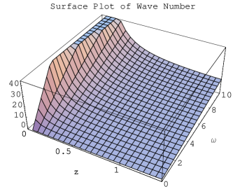
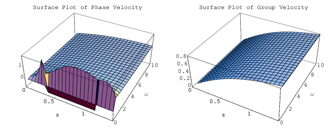
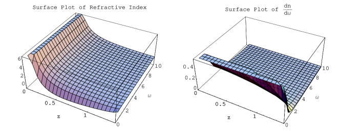
Figure 1: The waves decrease as they move away from the event horizon. The phase and the group velocities are equal except for the waves with less angular frequencies. The region shows normal dispersion.

We see from the Figure 1 that angular frequency $\omega$ and wave number $k$ are directly proportional to each other, i.e., the change in angular velocity gives the respective change in wave number. Also, the wave number decreases as $z$ increases. This means that waves lose energy as we go away from the black hole horizon. At the horizon, the wave number becomes very large and the waves vanish due to the effect of gravity. There is an abrupt increment in phase velocity when the angular frequency is near to zero. The region $3.5\times 10^{-7}\leq z\leq 0.5,~{}1.5\leq\omega\leq 10$ has refractive index greater than one and its variation with respect to omega greater than zero. This corresponds to the region of normal dispersion [30]. The group and wave velocities go parallel and are increasing as we go away from the horizon.

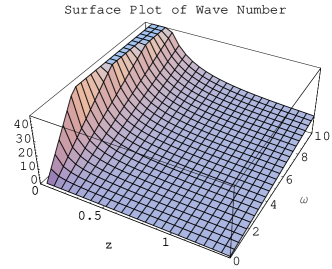
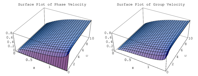
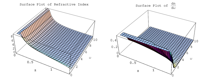
Figure 2: The waves damp as they go away from the event horizon. The phase and the group velocities are equal except for the waves with negligible angular frequencies. The region shows normal dispersion.

The Figure 2 shows that the waves are growing with the increase in angular velocity, but damping occurs with as $z$ increases. For $0\leq z<3.5\times 10^{-7}$, the wave number goes to infinity and hence there is no wave at the horizon. This shows that the event horizon is the interface at which they are formed and as we go away from the event horizon, the intensity of these waves decay. Since the refractive index is greater than one and $\frac{dn}{d\omega}$ is greater than zero, the whole region shows normal dispersion.

The dispersion equation obtained from the imaginary part of the matrix is of the form $A(z)k+B(z)\omega=0.$ Hence we are with only one value of $k$ given by the Figure 3.

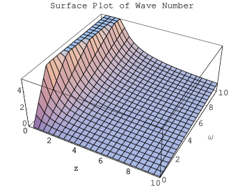
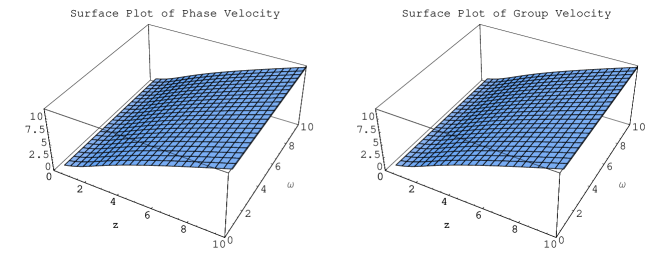
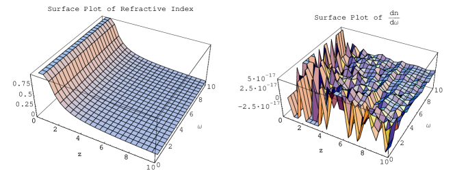
Figure 3: The waves damp as they move away from the event horizon. The phase and the group velocities are same. The dispersion is not normal.

The Figure 3 shows that the waves gain energy with the increase in angular velocity, but lose as $z$ increases. The wave number goes to infinity and hence there is no wave for $0\leq z<3.5\times 10^{-7}$. The group and phase velocities are showing the same behavior i.e. they are increasing with an increase in $z$. The refractive index is not greater than one and hence the dispersion is not normal.

4 Rotating Non-Magnetized Background

When we consider non-magnetized cold plasma in rotating background, i.e., $\textbf{B}=0$, the GRMHD Eqs.(2.17) and (2.18) vanish. Eqs.(2.19) and (2.20) change into general relativistic hydrodynamical equations given below:

$$\frac{\partial\rho}{\partial t}+(\alpha\textbf{V}.\nabla)\rho+\rho\gamma^{2}\textbf{V}.\frac{\partial\textbf{V}}{\partial t}+\rho\gamma^{2}\textbf{V}.(\alpha\textbf{V}.\nabla)\textbf{V}+\rho\nabla.(\alpha\textbf{V})=0,$$ ( 4. 1)

$$(\rho\gamma^{2}\delta_{ij}+\rho\gamma^{4}V_{i}V_{j})\left(\frac{1}{\alpha}\frac{\partial}{\partial t}+\textbf{V}.\nabla\right)V^{j}=-\rho\gamma^{2}a_{i}.$$ ( 4. 2)

For rotating background, the fluid four-velocity measured by FIDO can be described in $xz$-plane as follows

$$\textbf{V}=V(z)\textbf{e}_{\textbf{x}}+u(z)\textbf{e}_{\textbf{z}}$$ ( 4. 3)

and the Lorentz factor $\gamma$ takes the form

$$\gamma=\frac{1}{\sqrt{1-u^{2}-V^{2}}}.$$ ( 4. 4)

Here we shall use the following notations for the perturbed quantities

$$\tilde{\rho} \equiv \frac{\delta\rho}{\rho}=\tilde{\rho}(t,z)$$

v $$\equiv \delta\textbf{V}=\textbf{v}_{\textbf{x}}(t,z)\textbf{e}_{\textbf{x}}+\textbf{v}_{\textbf{z}}(t,z)\textbf{e}_{\textbf{z}}$$ ( 4. 5)

and the perturbations have harmonic space and time dependence, i.e.,

$$\tilde{\rho},~{}\textbf{v}\sim e^{-i(\omega t-kz)}.$$ ( 4. 6)

The perturbed variables take the form

$$\tilde{\rho}(t,z)=c_{1}e^{-\iota(\omega t-kz)},$$

$$\textbf{v}_{\textbf{z}}(t,z)=c_{2}e^{-\iota(\omega t-kz)},$$

$$\textbf{v}_{\textbf{x}}(t,z)=c_{3}e^{-\iota(\omega t-kz)}.$$ ( 4. 7)

4.1 Perturbation Equations

Introducing linear perturbations in Eqs.(4.1) and (4.2), it follows that

$$\left(\frac{1}{\alpha}\frac{\partial}{\partial t}+\textbf{V}.\nabla\right)\delta\rho+\rho\gamma^{2}\textbf{V}.\left(\frac{1}{\alpha}\frac{\partial}{\partial t}+\textbf{V}.\nabla\right)\textbf{v}-\frac{\delta\rho}{\rho}(\textbf{V}.\nabla)\rho+\rho(\nabla.\textbf{v})$$

$$=-2\rho\gamma^{2}(\textbf{V}.\textbf{v})(\textbf{V}.\nabla)ln\gamma-\rho\gamma^{2}(\textbf{V}.\nabla\textbf{V}).\textbf{v}+\rho(\textbf{v}.\nabla lnu),$$ ( 4. 8)

$$(\rho\gamma^{2}\delta_{ij}+\rho\gamma^{4}V_{i}V_{j})\frac{1}{\alpha}\frac{\partial v^{j}}{\partial t}+\rho\gamma^{2}v_{i,j}V^{j}+\rho\gamma^{4}V_{i}v_{j,k}V^{j}V^{k}=-\gamma^{2}\{\delta\rho+2\rho\gamma^{2}(\textbf{V}.\textbf{v})\}a_{i}$$

$$-\rho\gamma^{4}(v_{i}V^{j}+v^{j}V_{i})V_{k,j}V^{k}-\gamma^{2}\{\delta\rho V^{j}+2\rho\gamma^{2}(\textbf{V}.\textbf{v})V^{j}+\rho v^{j}\}V_{i,j}$$

$$-\gamma^{4}V_{i}\{\delta\rho V^{j}+4\rho\gamma^{2}(\textbf{V}.\textbf{v})V^{j}+\rho v^{j}\}V_{j,k}V^{k}.$$ ( 4. 9)

The component form of Eqs.(4.8) and (4.9) gives the following three equations

$$\frac{1}{\alpha}\frac{\partial\tilde{\rho}}{\partial t}+u\tilde{\rho}_{,z}+\gamma^{2}V\left(\frac{1}{\alpha}\frac{\partial v_{x}}{\partial t}+uv_{x,z}\right)+\gamma^{2}u\frac{1}{\alpha}\frac{\partial v_{z}}{\partial t}+(1+\gamma^{2}u^{2})v_{z,z}$$

$$=-\gamma^{2}u\{(1+2\gamma^{2}V^{2})V^{\prime}+2\gamma^{2}uVu^{\prime}\}v_{x}+\left\{(1-2\gamma^{2}u^{2})(1+\gamma^{2}u^{2})\frac{u^{\prime}}{u}-2\gamma^{4}u^{2}VV^{\prime}\right\}v_{z},$$ ( 4. 10)

$$\gamma^{2}(1+\gamma^{2}V^{2})\left(\frac{1}{\alpha}\frac{\partial v_{x}}{\partial t}+uv_{x,z}\right)+\gamma^{4}uV(\frac{1}{\alpha}\frac{\partial v_{z}}{\partial t}+uv_{z,z})$$

$$=-\tilde{\rho}\gamma^{2}u\{(1+\gamma^{2}V^{2})V^{\prime}+\gamma^{2}uVu^{\prime}\}-\gamma^{4}u\{(1+4\gamma^{2}V^{2})uu^{\prime}+4VV^{\prime}(1+\gamma^{2}V^{2})\}v_{x}$$

$$-[\gamma^{2}\{(1+2\gamma^{2}u^{2})(1+2\gamma^{2}V^{2})-\gamma^{2}V^{2}\}V^{\prime}+2\gamma^{4}(1+2\gamma^{2}u^{2})uVu^{\prime}]v_{z},$$ ( 4. 11)

$$\gamma^{2}(1+\gamma^{2}u^{2})\left(\frac{1}{\alpha}\frac{\partial v_{z}}{\partial t}+uv_{z,z}\right)+\gamma^{4}uV\left(\frac{1}{\alpha}\frac{\partial v_{x}}{\partial t}+uv_{x,z}\right)$$

$$=-\tilde{\rho}\gamma^{2}\{a_{z}+(1+\gamma^{2}u^{2})uu^{\prime}+\gamma^{2}u^{2}VV^{\prime}\}$$

$$-[\gamma^{4}\{u^{2}V^{\prime}(1+4\gamma^{2}V^{2})+2V(a_{z}+(1+2\gamma^{2}u^{2})uu^{\prime})\}]v_{x}$$

$$-\gamma^{2}[u^{\prime}(1+\gamma^{2}u^{2})(1+4\gamma^{2}u^{2})+2u\gamma^{2}\{a_{z}+(1+2\gamma^{2}u^{2})VV^{\prime}\}]v_{z}.$$ ( 4. 12)

Using Eq.(4.7), the Fourier analyzed form of Eqs.(4.10)-(4.12) become

$$c_{1}\left(-\frac{\iota\omega}{\alpha}+\iota ku\right)+c_{2}\left[-\frac{\iota\omega}{\alpha}\gamma^{2}u+(1+\gamma^{2}u^{2})\iota k-(1-2\gamma^{2}u^{2})(1+\gamma^{2}u^{2})\frac{u^{\prime}}{u}+2\gamma^{4}u^{2}VV^{\prime}\right]$$

$$+c_{3}\gamma^{2}\left[-\frac{\iota\omega}{\alpha}V+\iota kuV+\gamma^{2}u\{(1+2\gamma^{2}V^{2})V^{\prime}+2\gamma^{2}uVu^{\prime}\}\right]=0,$$ ( 4. 13)

$$c_{1}\gamma^{2}u\{(1+\gamma^{2}V^{2})V^{\prime}+\gamma^{2}uVu^{\prime}\}+c_{2}\gamma^{2}[\left(-\frac{\iota\omega}{\alpha}+\iota ku\right)\gamma^{2}uV$$

$$+\{(1+2\gamma^{2}u^{2})(1+2\gamma^{2}V^{2})-\gamma^{2}V^{2}\}V^{\prime}+2\gamma^{2}(1+2\gamma^{2}u^{2})uVu^{\prime}]$$

$$+c_{3}[\left(-\frac{\iota\omega}{\alpha}+\iota ku\right)\gamma^{2}(1+\gamma^{2}V^{2})+\gamma^{4}u\{(1+4\gamma^{2}V^{2})uu^{\prime}+4VV^{\prime}(1+\gamma^{2}V^{2})\}]=0,$$ ( 4. 14)

$$c_{1}\gamma^{2}\{a_{z}+(1+\gamma^{2}u^{2})uu^{\prime}+\gamma^{2}u^{2}VV^{\prime}\}+c_{2}[\gamma^{2}(1+\gamma^{2}u^{2})\left(-\frac{\iota\omega}{\alpha}+\iota uk\right)$$

$$+\gamma^{2}\{u^{\prime}(1+\gamma^{2}u^{2})(1+4\gamma^{2}u^{2})+2u\gamma^{2}(a_{z}+(1+2\gamma^{2}u^{2})VV^{\prime})\}]$$

$$+c_{3}\gamma^{4}\left[\left(-\frac{\iota\omega}{\alpha}+\iota uk\right)uV+u^{2}V(1+4\gamma^{2}V^{2})+2V\{a_{z}+uu^{\prime}(1+2\gamma^{2}u^{2})\}\right]=0.$$ ( 4. 15)

The determinant of the coefficients of $c_{1},~{}c_{2}$ and $c_{3}$ gives a complex number. Equating it to zero yields a complex dispersion relation in $k$.

4.2 Numerical Solutions

We consider time lapse $\alpha=z$ and assume that $V=u$ for the sake of convenience. Using mass conservation law in three dimensions (with mass density as a constant quantity) we obtain $u=\frac{1}{\sqrt{2+z^{2}}}.$ In this section we are having modes when $\textbf{B}=0$. The complex dispersion relation obtained from the determinant of coefficients leads to two dispersion equations. The real part gives an equation of the type $A(z)k^{2}+B(z)k\omega+C(z)\omega^{2}+D(z)=0$ leading to two dispersion relations shown in the Figures 4 and 5. The imaginary part shows a cubic equation $A(z)k^{3}+B(z)k^{2}\omega+C(z)k\omega^{2}+D(z)\omega^{3}=0.$ This equation has one real and two complex conjugate solutions. The Figure 6 shows the real value of $k$ obtained from this equation.

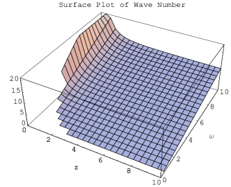
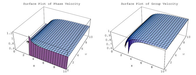
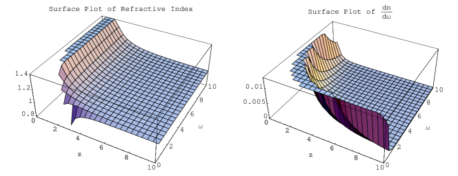
Figure 4: The waves damp when they move away from the event horizon. The phase velocity is less than the group velocity in most of the region. Most of the region shows normal dispersion.

The Figure 4 indicates that the region for which real waves exist lies in $1.5\times 10^{-8}<z\leq 10,~{}0.045<\omega\leq 10$. It is clear from the Figure that the region $0<\omega\leq 0.045$ contains evanescent waves. We note that at the horizon and nearby values of $z$ i.e. in the region $0\leq z\leq 1.5\times 10^{-8}$, the wave number is infinite and hence no wave exists there. The wave number is decreasing as we go away from the horizon and hence damping occurs. Also $n>1,~{}\frac{dn}{d\omega}>0$ and hence the region is of normal dispersion. The phase velocity is less than group velocity of waves except at some points where the refractive index $n$ is positive but is less than one, as shown in the graph. This means that the dispersion is not normal but anomalous at these points [31], normal otherwise. At $\omega=0$ and very small angular frequencies, the phase velocity is high but the group velocity become infinite which is not physical.

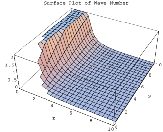
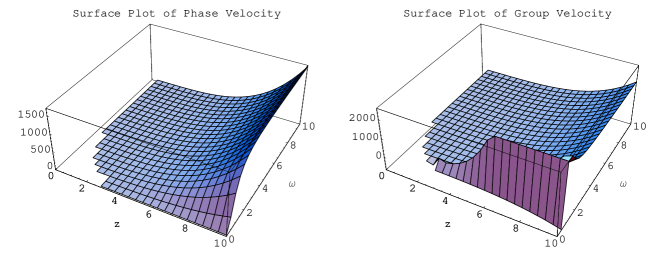
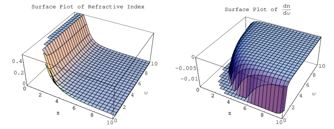
Figure 5: The waves damp while they move away from the event horizon. The dispersion is not normal.

The Figure 5 contains the infinite wave number in the region $0\leq z<1.5\times 10^{-8}$, that is no wave present there. The wave number possesses real values in the region $1.5\times 10^{-8}<z\leq 10,~{}0.05\leq\omega\leq 10$. On increasing the value of $z$, the waves are damping but are growing with the increase of the angular frequency. In this region, refractive index $n<1$ and $\frac{dn}{d\omega}<0$ which implies that the region is not of normal dispersion. At $1.5\times 10^{-8}<z\leq 10,~{}0\leq\omega\leq 4$, the wave number becomes imaginary at several points leading to the result that evanescent waves present there.

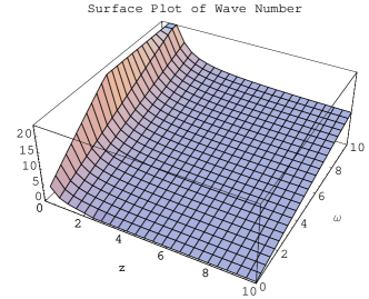
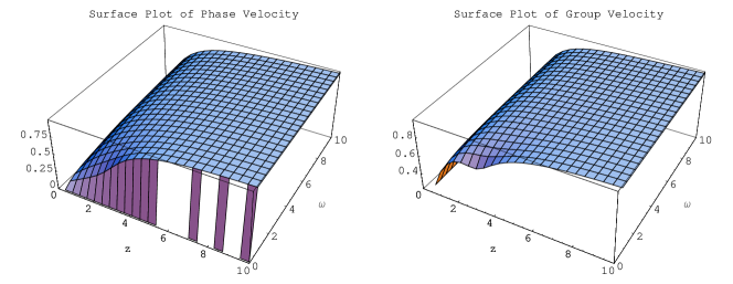
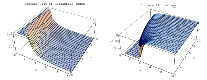
Figure 6: The waves damp as they move away from the event horizon. The group velocity is greater than the phase velocity. The region is of anomalous dispersion.

In the Figure 6, real waves exist in the region $1.5\times 10^{-8}\leq z\leq 10.$ The refractive index is greater than one, $\frac{dn}{d\omega}$ is negative and thus the region is not of normal dispersion. No wave is present on the event horizon because the wave number is infinite there. As we go away from the horizon, the wave number decreases. On increasing the angular frequency, we find growing waves. Also, group velocity is greater than phase velocity which indicates that the region is of anomalous dispersion.

5 Rotating Magnetized Background

The GRMHD equations for magnetized cold plasma in rotating background will remain the same as given by Eqs.(2.17)-(2.20). Here the four-velocity of the fluid measured by FIDO can be described in the same way as given in the previous section. The rotating magnetic field can be expressed in the $xz$-plane as

$${}\textbf{B}=B[\lambda(z)\textbf{e}_{\textbf{x}}+\textbf{e}_{\textbf{z}}],$$ ( 5. 1)

where $\lambda,~{}u$ and $V$ are related to each other by

$$V=\frac{V_{F}}{\alpha}+\lambda u,$$ ( 5. 2)

$V_{F}$ as an integration constant. The following notations for the perturbed magnetic field will be used in addition to the notations given by Eq.(4.5).

b $$\equiv \frac{\delta\textbf{B}}{B}=\textbf{b}_{\textbf{x}}(t,z)\textbf{e}_{\textbf{x}}+\textbf{b}_{\textbf{z}}(t,z)\textbf{e}_{\textbf{z}}.$$ ( 5. 3)

Since the perturbations have harmonic space and time dependence, i.e., $\textbf{b}\sim e^{-i(\omega t-kz)}$, the perturbed variable can be expressed as follows

$$\textbf{b}_{\textbf{x}}(t,z)=c_{4}e^{-\iota(\omega t-kz)},$$

$$\textbf{b}_{\textbf{z}}(t,z)=c_{5}e^{-\iota(\omega t-kz)}.$$ ( 5. 4)

5.1 Perturbation Equations

Using Eq.(2.21) in Eqs.(2.17)-(2.20), we have

$$\frac{\partial(\delta\textbf{B})}{\partial t}=\nabla\times(\alpha\textbf{v}\times\textbf{B})+\nabla\times(\alpha\textbf{V}\times\delta\textbf{B}),$$ ( 5. 5)

$$\nabla.(\delta\textbf{B})=0,$$ ( 5. 6)

$$\left(\frac{1}{\alpha}\frac{\partial}{\partial t}+\textbf{V}.\nabla\right)\delta\rho+\rho\gamma^{2}\textbf{V}.\left(\frac{1}{\alpha}\frac{\partial}{\partial t}+\textbf{V}.\nabla\right)\textbf{v}-\frac{\delta\rho}{\rho}(\textbf{V}.\nabla)\rho+\rho(\nabla.\textbf{v})$$

$$=-2\rho\gamma^{2}(\textbf{V}.\textbf{v})(\textbf{V}.\nabla)ln\gamma-\rho\gamma^{2}(\textbf{V}.\nabla\textbf{V}).\textbf{v}+\rho(\textbf{v}.\nabla lnu),$$ ( 5. 7)

$$\left\{\left(\rho\gamma^{2}+\frac{\textbf{B}^{2}}{4\pi}\right)\delta_{ij}+\rho\gamma^{4}V_{i}V_{j}-\frac{1}{4\pi}B_{i}B_{j}\right\}\frac{1}{\alpha}\frac{\partial v^{j}}{\partial t}+\frac{1}{4\pi}\left[\textbf{B}\times\left\{\textbf{V}\times\frac{1}{\alpha}\frac{\partial(\delta\textbf{B})}{\partial t}\right\}\right]_{i}$$

$$+\rho\gamma^{2}v_{i,j}V^{j}+\rho\gamma^{4}V_{i}v_{j,k}V^{j}V^{k}-\frac{1}{4\pi\alpha}\{(\alpha\delta B_{i})_{,j}-(\alpha\delta B_{j})_{,i}\}B^{j}=-\gamma^{2}\{\delta\rho+2\rho\gamma^{2}(\textbf{V}.\textbf{v})\}a_{i}$$

$$+\frac{1}{4\pi\alpha}\{(\alpha B_{i})_{,j}-(\alpha B_{j})_{,i}\}\delta B^{j}-\rho\gamma^{4}(v_{i}V^{j}+v^{j}V_{i})V_{k,j}V^{k}-\gamma^{2}\{\delta\rho V^{j}+2\rho\gamma^{2}(\textbf{V}.\textbf{v})V^{j}+\rho v^{j}\}V_{i,j}$$

$$-\gamma^{4}V_{i}\{\delta\rho V^{j}+4\rho\gamma^{2}(\textbf{V}.\textbf{v})V^{j}+\rho v^{j}\}V_{j,k}V^{k}.$$ ( 5. 8)

The component form of the Eqs.(5.5)-(5.8) can be written, after a tedious algebra, as follows

$$\frac{1}{\alpha}\frac{\partial b_{x}}{\partial t}+ub_{x,z}=\nabla ln\alpha(v_{x}-\lambda v_{z}+Vb_{z}-ub_{x})+(v_{x,z}-\lambda v_{z,z}-\lambda^{\prime}v_{z}+V^{\prime}b_{z}-u^{\prime}b_{x}),$$ ( 5. 9)

$$\frac{1}{\alpha}\frac{\partial b_{z}}{\partial t}+ub_{z,z}=0,$$ ( 5. 10)

$$b_{z,z}=0,$$ ( 5. 11)

$$\frac{1}{\alpha}\frac{{\partial\tilde{\rho}}}{\partial t}+u\tilde{\rho}_{,z}+\gamma^{2}V\frac{1}{\alpha}\frac{\partial v_{x}}{\partial t}+\gamma^{2}u\frac{1}{\alpha}\frac{\partial v_{z}}{\partial t}+(1+\gamma^{2}u^{2})v_{z,z}+\gamma^{2}uVv_{x,z}$$

$$=-\gamma^{2}u[(1+2\gamma^{2}V^{2})V^{\prime}+2\gamma^{2}uVu^{\prime}]v_{x}+[(1-2\gamma^{2}u^{2})(1+\gamma^{2}u^{2})\frac{u^{\prime}}{u}-2\gamma^{4}u^{2}VV^{\prime}]v_{z},$$ ( 5. 12)

$$\left\{\rho\gamma^{2}(1+\gamma^{2}V^{2})+\frac{B^{2}}{4\pi}\right\}\frac{1}{\alpha}\frac{\partial v_{x}}{\partial t}+\left(\rho\gamma^{4}uV-\frac{\lambda B^{2}}{4\pi}\right)\frac{1}{\alpha}\frac{\partial v_{z}}{\partial t}+\left\{\rho\gamma^{2}(1+\gamma^{2}V^{2})-\frac{B^{2}}{4\pi}\right\}uv_{x,z}$$

$$+\left(\rho\gamma^{4}uV+\frac{\lambda B^{2}}{4\pi}\right)uv_{z,z}-\frac{B^{2}}{4\pi}(1-u^{2})b_{x,z}-\frac{B^{2}}{4\pi\alpha}b_{x}\{\alpha^{\prime}(1-u^{2})-\alpha uu^{\prime}\}$$

$$+\tilde{\rho}\rho\gamma^{2}u\{(1+\gamma^{2}V^{2})V^{\prime}+\gamma^{2}uVu^{\prime}\}+\left[\rho\gamma^{4}u\{(1+4\gamma^{2}V^{2})uu^{\prime}+4(1+\gamma^{2}V^{2})VV^{\prime}\}+\frac{B^{2}u\alpha^{\prime}}{4\pi\alpha}\right]v_{x}$$

$$+\left[\rho\gamma^{2}[\{(1+2\gamma^{2}u^{2})(1+2\gamma^{2}V^{2})-\gamma^{2}V^{2}\}V^{\prime}+2\gamma^{2}(1+2\gamma^{2}u^{2})uVu^{\prime}]+\frac{B^{2}u}{4\pi\alpha}(\lambda\alpha)^{\prime}\right]v_{z}=0,$$ ( 5. 13)

$$\left\{\rho\gamma^{2}(1+\gamma^{2}u^{2})+\frac{\lambda^{2}B^{2}}{4\pi}\right\}\frac{1}{\alpha}\frac{\partial v_{z}}{\partial t}+\left(\rho\gamma^{4}uV-\frac{\lambda B^{2}}{4\pi}\right)\frac{1}{\alpha}\frac{\partial v_{x}}{\partial t}+\left\{\rho\gamma^{2}(1+\gamma^{2}u^{2})-\frac{\lambda^{2}B^{2}}{4\pi}\right\}uv_{z,z}$$

$$+\left(\rho\gamma^{4}uV+\frac{\lambda B^{2}}{4\pi})uv_{x,z}\right)+\frac{\lambda B^{2}}{4\pi}(1-u^{2})b_{x,z}+\frac{B^{2}}{4\pi\alpha}\{(\alpha\lambda)^{\prime}+\alpha^{\prime}\lambda-u\lambda(u\alpha^{\prime}+u^{\prime}\alpha)\}b_{x}$$

$$+\tilde{\rho}\gamma^{2}[a_{z}+u\{(1+\gamma^{2}u^{2})u^{\prime}+\gamma^{2}uVV^{\prime}\}]$$

$$+\left[\rho\gamma^{4}\{u^{2}V^{\prime}(1+4\gamma^{2}V^{2})+2V(a_{z}+uu^{\prime}(1+2\gamma^{2}u^{2}))\}+\frac{\lambda B^{2}\alpha^{\prime}u}{4\pi\alpha}\right]v_{x}$$

$$+\left[\rho\gamma^{2}\{u^{\prime}(1+\gamma^{2}u^{2})(1+4\gamma^{2}u^{2})+2u\gamma^{2}\{(1+2\gamma^{2}u^{2})VV^{\prime}+a_{z}\}\}-\frac{\lambda B^{2}u}{4\pi\alpha}(\alpha\lambda)^{\prime}\right]v_{z}=0.$$ ( 5. 14)

When the above equations are Fourier analyzed, they take the following form

$$c_{3}(\alpha^{\prime}+\iota k\alpha)-c_{2}\{(\alpha\lambda)^{\prime}+\iota k\alpha\lambda\}+c_{5}(\alpha V)^{\prime}-c_{4}\{(\alpha u)^{\prime}-\iota\omega+\iota k\alpha u\}=0,$$ ( 5. 15)

$$c_{5}\left(-\frac{\iota\omega}{\alpha}+\iota ku\right)=0,$$ ( 5. 16)

$$c_{5}\iota k=0,$$ ( 5. 17)

$$c_{1}\left(-\frac{\iota\omega}{\alpha}+\iota ku\right)+c_{2}\left\{-\frac{\iota\omega}{\alpha}\gamma^{2}u+\iota k(1+\gamma^{2}u^{2})-(1-2\gamma^{2}u^{2})(1+\gamma^{2}u^{2})\frac{u^{\prime}}{u}+2\gamma^{4}u^{2}VV^{\prime}\right\}$$

$$+c_{3}\gamma^{2}\left[\left(-\frac{\iota\omega}{\alpha}+\iota ku\right)V+u\{(1+2\gamma^{2}V^{2})V^{\prime}+2\gamma^{2}uVu^{\prime}\}\right]=0,$$ ( 5. 18)

$$c_{1}\rho\gamma^{2}u\{(1+\gamma^{2}V^{2})V^{\prime}+\gamma^{2}uVu^{\prime}\}-\frac{B^{2}}{4\pi}c_{4}\{(1-u^{2})\iota k+\frac{\alpha^{\prime}}{\alpha}(1-u^{2})-uu^{\prime}\}$$

$$+c_{2}\left[-\left(\rho\gamma^{4}uV-\frac{\lambda B^{2}}{4\pi}\right)\frac{\iota\omega}{\alpha}+\iota ku\left(\rho\gamma^{4}uV+\frac{\lambda B^{2}}{4\pi}\right)+\rho\gamma^{2}\{(1+2\gamma^{2}u^{2})(1+2\gamma^{2}V^{2})-\gamma^{2}V^{2}\}V^{\prime}\right.$$

$$\left.+2\rho\gamma^{4}(1+2\gamma^{2}u^{2})uVu^{\prime}+\frac{B^{2}u}{4\pi\alpha}(\lambda\alpha)^{\prime}\right]+c_{3}\left[-\left\{\rho\gamma^{2}(1+\gamma^{2}V^{2})+\frac{B^{2}}{4\pi}\right\}\frac{\iota\omega}{\alpha}\right.$$

$$\left.+\iota ku\left\{\rho\gamma^{2}(1+\gamma^{2}V^{2})-\frac{B^{2}}{4\pi}\right\}+\rho\gamma^{4}u\{(1+4\gamma^{2}V^{2})uu^{\prime}+4(1+\gamma^{2}V^{2})VV^{\prime}\}-\frac{B^{2}u\alpha^{\prime}}{4\pi\alpha}\right]=0,$$ ( 5. 19)

$$c_{1}\rho\gamma^{2}[a_{z}+u\{(1+\gamma^{2}u^{2})u^{\prime}+\gamma^{2}VuV^{\prime}\}]$$

$$+c_{2}\left[-\left\{\rho\gamma^{2}(1+\gamma^{2}u^{2})+\frac{\lambda^{2}B^{2}}{4\pi}\right\}\frac{\iota\omega}{\alpha}+\left\{\rho\gamma^{2}(1+\gamma^{2}u^{2})-\frac{\lambda^{2}B^{2}}{4\pi}\right\}\iota ku\right.$$

$$\left.+\left\{\rho\gamma^{2}\{u^{\prime}(1+\gamma^{2}u^{2})(1+4\gamma^{2}u^{2})+2u\gamma^{2}((1+2\gamma^{2}u^{2})VV^{\prime}+a_{z})\}-\frac{\lambda B^{2}u}{4\pi\alpha}(\alpha\lambda)^{\prime}\right\}\right]$$

$$+c_{3}\left[-\left(\rho\gamma^{4}uV-\frac{\lambda B^{2}}{4\pi}\right)\frac{\iota\omega}{\alpha}+\left(\rho\gamma^{4}uV+\frac{\lambda B^{2}}{4\pi}\right)\iota ku\right.$$

$$\left.+\left\{\rho\gamma^{4}\{u^{2}V^{\prime}(1+4\gamma^{2}V^{2})+2V(a_{z}+uu^{\prime}(1+2\gamma^{2}u^{2}))\}+\frac{\lambda B^{2}\alpha^{\prime}u}{4\pi\alpha}\right\}\right]$$

$$+\frac{B^{2}}{4\pi}c_{4}\left[\lambda(1-u^{2})\iota k+\lambda\frac{\alpha^{\prime}}{\alpha}(1-u^{2})-\lambda uu^{\prime}+\frac{(\lambda\alpha)^{\prime}}{\alpha}\right]=0.$$ ( 5. 20)

Equation (5.17) implies that $c_{5}$ is zero which gives that $b_{z}$ is zero.

5.2 Numerical Solutions

We consider the same circumstances as we have considered in the rotating non-magnetized plasma and assume that $u=\frac{1}{\sqrt{z^{2}+2}}=V$. Substituting this value in Eq.(5.2) with $V_{F}=1$, it follows that $\lambda=1-\frac{\sqrt{z^{2}+2}}{z}$ which shows that the magnetic field diverges near the horizon (as discussed in [25]). For the sake of convenience, we take $B=\sqrt{\frac{176}{7}}$ so that $\frac{B^{2}}{4\pi}=2$. Making use of $c_{5}=0$ (Eq.(5.17)), we get a $4\times 4$ matrix of the coefficients of constants. The complex dispersion relation has two parts. The real part gives a dispersion relation of the type $A(z)k^{4}+B(z)k^{3}\omega+C(z)\omega^{2}+D(z)\omega^{4}+E(z)k^{2}+F(z)k^{2}\omega^{2}+G(z)k\omega+H(z)k\omega^{2}+L(z)=0$ whereas the imaginary part gives a relation of the form $A(z)k^{3}+B(z)k^{2}\omega+C(z)\omega+D(z)\omega^{3}+E(z)k\omega^{2}+F(z)k=0.$ The first equation gives four dispersion relations out of which two are real and interesting while the other two roots are complex conjugates of each other. The second equation gives three dispersion relations. The respective wave numbers are shown in the Figures 9-11. These relations give different types of modes when $\textbf{B}>0$ and wave number is in arbitrary direction to $\textbf{B}.$ The two dispersion relations obtained from the real part are shown in the Figures 7 and 8.

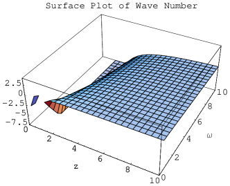
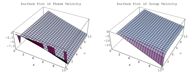
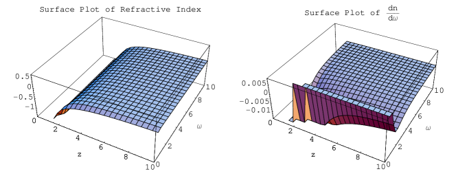
Figure 7: The waves grow as they move away from the event horizon. The medium admits the properties of metamaterials.

The Figure 7 shows that at the horizon the wave number is infinite and hence no wave is present there. $k$ has real values in the region $1\leq z\leq 10,~{}10^{-7}\leq\omega\leq 10$. No wave is present in the region $0\leq z<1$, evanescent waves are present in $0\leq\omega<10^{-7}.$ All the quantities, the wave number, wave velocity, group velocity and refractive index are negative. This leads to the existence of metamaterial in the region [32]. The wave number is decreasing with an increase in angular frequency and increasing with an increase in time lapse.

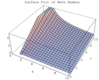
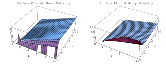
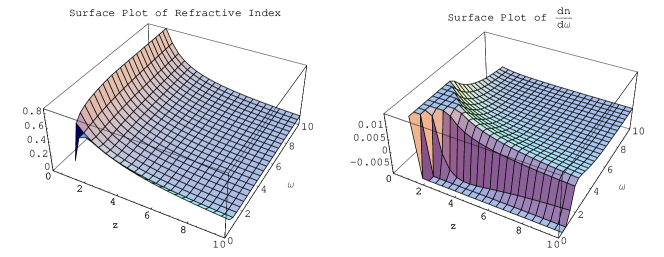
Figure 8: The waves damp as they move away from the event horizon. The dispersion is not normal in the region.

The Figure 8 shows that the wave number increases with the increase in angular velocity and decreases with the increase of lapse function. The horizon possesses no wave due to infinite wave number. The region $0<z\leq 1$ has no wave and $0\leq\omega<5\times 10^{-6}$ is region of evanescent waves. The value of refractive index is less than one and hence it is not a normal dispersion.

The dispersion relation obtained from the imaginary part of the matrix determinant are shown in the Figures 9, 10 and 11.

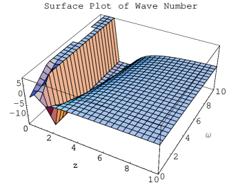
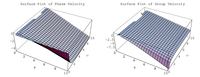
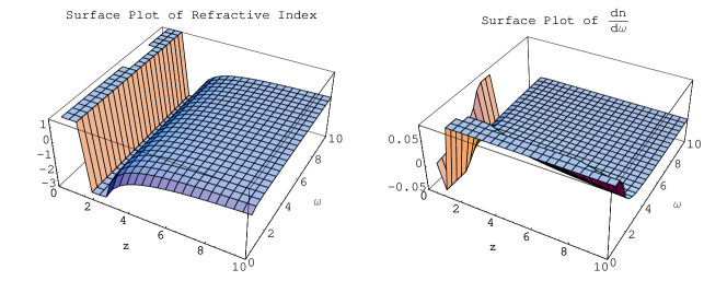
Figure 9: The waves damp and then grow as they move away from the event horizon. The medium admits the properties of metamaterials.

The Figure 9 shows that the wave number is infinite in $0\leq z<0.5.$ The wave number is positive in the region $0.5\leq z<1.6$, it decreases abruptly and then it smoothly rises but is negative. The phase and group velocities are negative. The refractive index is negative in the domain $1.6\leq z<10$ so the region possesses the properties of metamaterials.

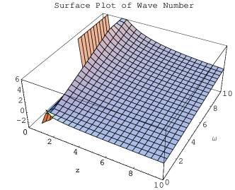
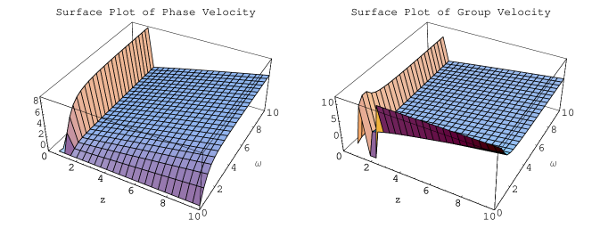
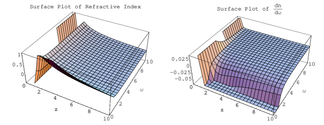
Figure 10: The waves suddenly grow and then damp on going away from the event horizon. The dispersion is not normal.

In the Figure 10, real waves exist in the region $0.5\leq z\leq 10.$ No wave is present on the event horizon as well as in the region $0<z\leq 0.5$ because the wave number goes to infinity there. The waves are increasing in $0.5\leq z<0.7$ then there is a sudden decrease. The region $0.5\leq z\leq 0.7,~{}0\leq\omega<4$ contains evanescent waves. The refractive index is less than one in the whole domain, hence the waves are not normally disperse.

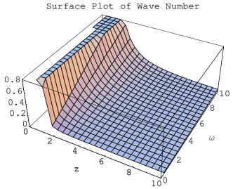
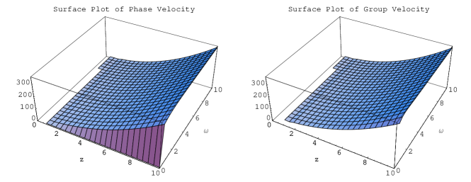
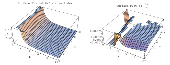
Figure 11: The waves damp when they move away from the event horizon. The phase and the group velocities are equal. The dispersion is not normal.

The Figure 11 shows that real waves exist in the region $0.5\leq z\leq 10,~{}0.5\leq\omega\leq 10.$ The phase and group velocities are same in this domain. The refractive index is less than one and the dispersion is not normal. No wave is present on the event horizon and the region near the horizon because the wave number is infinite there. As we go away from the horizon, the wave number decreases. On increasing the angular frequency, we find growing waves.

6 Conclusion

We have reformulated the GRMHD equations for the Schwarzschild black hole magnetosphere to take account of gravitational effects due to event horizon. We discuss one dimensional perturbations in perfect MHD condition. This has been explored for the cold plasma case. These equations are written in component form to make them easier for the Fourier analysis. The equations are Fourier analyzed by using the assumption of plane wave. The determinant of the coefficients is solved numerically for the following backgrounds in the magnetosphere.

1. Non-Rotating Background (either non-magnetized or magnetized)

2. Rotating Non-Magnetized Background

3. Rotating Magnetized Background.

The non-rotating background shows pure Schwarzschild geometry outside the event horizon whereas the rotating background demonstrates the restricted Kerr geometry in the vicinity of the event horizon which admits a variable lapse function with negligible rotation. We have taken Schwarzschild black hole with rotating background due to the well-known fact that the Schwarzschild black hole is the minimum configuration of the Kerr black hole.

In the case of non-rotating background, we have found that the magnetospheric fluid is normally disperse. The wave number becomes indefinite at the horizon and for the values of $z$ near the horizon and hence no wave is present there. This shows that no signal can pass the event horizon or near to it. The third subcase shows a mode which is not normally dispersive.

In the case of rotating non-magnetized background we have found one case (Figure 4) in which the dispersion is normal. The regions with zero angular frequency or very less angular frequency are evanescent in all the three cases. The wave number becomes infinite at event horizon and in the neighborhood of the event horizon and no wave exists there.

In rotating magnetized background, we obtain region with negative wave number, phase velocity, group velocity and refractive index (Figures 7 and 9). This fact is deduced by the analysis of two of the dispersion relations obtained in section 5. The refractive index is negative in both the cases which implies that the region possesses all the qualities of left-handed metamaterials. The other three dispersion relations give that the region under discussion is of non-normal dispersion which restrict the real signals pass through that region.

It is worth mentioning that the wave number becomes infinite at the event horizon and no wave exists there. This supports the well-known point of view that no information can be extracted from a black hole. It is interesting to mention that this work extends the results given by Mackay et al. in [33] according to which rotation of a black hole is required for negative phase velocity propagation. It is also observed that the waves of less angular velocity are evanescent. Our numerical results indicate that negative phase velocity propagates in the rotating background whether the black hole is rotating or non-rotating.

We know that the MHD waves in cold plasma are non-dispersive. However, the dispersion is noted in the above figures. This factor comes due to the formalism used and the equations which provides different equations from the usual MHD equations. Since the 3+1 split of GR is used in a preliminary investigation of waves propagating in a plasma influenced by the gravitational field. Thus internal gravity waves which interrupt the MHD waves imply the cases of dispersion in each of the hypersurface. We would like to mention that graphs of the waves are given in a particular hypersurface where time is constant, not in the whole Schwarzschild background and consequently this is justified locally, not globally. Finally, it is mentioned that some of the Figures have patches missing which is due to the existence of complex numbers there. Mathematica cannot plot complex numbers with real numbers. These complex numbers are shown by gaps in the Figures.

This analysis has been done for the cold plasma state. It would be interesting to extend this analysis for the isothermal state of plasma. This would provide the effects of pressure in the current work. Currently, it is in progress.

Acknowledgment

We acknowledge the enabling role of the Higher Education Commission Islamabad, Pakistan, and appreciate its financial support through the Indigenous PhD 5000 Fellowship Program Batch-II.

References

- [1] Petterson, J.A.: Phys. Rev. D10(1974)3166.
- [2] Israel, W.: Phys. Rev. 164(1967)1776; Commun. Math. Phys. 8(1968)245.
- [3] Hawking, S.: Commun. Math. Phys. 25(1972)152.
- [4] Robinson, D.: Phys. Rev. D10(1974)458.
- [5] Arnowitt, R., Deser, S. and Misner, C.W.: Gravitation: An Introduction to Current Research (Wiley, New York, 1962).
- [6] Tarfulea, N.: Ph.D. Thesis. (University of Minnesota, 2004).
- [7] Thorne, K.S. and Macdonald, D.A.: Mon. Not. R. astr. Soc. 198(1982)339.
- [8] Thorne, K.S. and Macdonald, D.A.: Mon. Not. R. astr. Soc.198(1982)345.
- [9] Thorne, K.S., Price, R.H. and Macdonald, D.A.: Black Holes: The Membrane Paradigm (Yale University Press, New Haven, 1986).
- [10] Holcomb, K.A. and Tajima, T.: Phys. Rev. D40(1989)3809.
- [11] Holcomb, K.A.: Astrophys. J. 362(1990)381.
- [12] Dettman, C.P., Frankel, N.E. and Kowalenko, V.: Phys. Rev. D48(1993)5655.
- [13] Khanna, R.: Mon. Not. R. Astr. Soc. 294(1998)673.
- [14] Antón, L., Zanotti, O., Miralles, J.A., Martí, J.A., Ibáez, J., Font, J.A. and Pons, J.A.: Astrophys. J. 637(2006)296.
- [15] Anile, A.M.: Relativistic Fluids and Magneto-Fluids with Applications in Astrophysics and Plasma Physics (Cambridge University Press, 1989).
- [16] Komissarov, S.S.: Mon. Not. R. Astron. Soc. 336(2002)759.
- [17] Komissarov, S.S.: Mon. Not. R. Astron. Soc. 350(2004)407.
- [18] Zhang, X.-H.: Phys. Rev. D39(1989)2933.
- [19] Zhang, X.-H.: Phys. Rev. D40(1989)3858.
- [20] Tsikarishvili, E.G., Rogava, A.D., Lominadze, J.G. and Javakhishvili, J.I.: Phys. Rev. A46(1992)1078.
- [21] Mofiz, U.A.: BRAC University Journal, II(2005)83.
- [22] Regge, T. and Wheeler, J.A.: Phys. Rev. 108(1957)1063.
- [23] Zerilli, F.: Phys. Rev. D2(1970)2141; J. Math. Phys. 11(1970)2203; Phys. Rev. Lett. 24(1970)737.
- [24] Price, R.H.: Phys. Rev. D5(1972)2419; ibid 2439.
- [25] Hanni, R.S. and Ruffini R.: Phys. Rev. D8(1973)3259.
- [26] Wald, R.M.: Phys. Rev. D10(1974)1680.
- [27] Sakai, J. and Kawata, T.: J. Phys. Soc. Jpn. 49(1980)747.
- [28] Buzzi, V., Hines, K.C. and Treumann, R.A.: Phys. Rev. D51(1995)6663; ibid 6677.
- [29] Das, A.C.: Space Plasma Physics: An Introduction (Narosa Publishing House, New Delhi, 2004).
- [30] Jackson, J.D.: Classical Electrodynamics (John Wiley & Sons, 1999).
- [31] Achenbach, J.D.: Wave Propogation in Elastic Solids (North-Holland Publishing Company, Oxford, 1973).
- [32] Veselago, V.G.: Sov. Phys. Usp. 10(1968)509.
- [33] Mackay, T.G., Lakhtakia, A. and Setiawan, S.: New J. Phys. 7(2005)171.