The bends on a quantum waveguide and cross-products of Bessel functions

Abstract

A detailed analysis of the wave-mode structure in a bend and its incorporation into a stable algorithm for calculation of the scattering matrix of the bend is presented. The calculations are based on the modal approach. The stability and precision of the algorithm is numerically and analytically analysed. The algorithm enables precise numerical calculations of scattering across the bend. The reflection is a purely quantum phenomenon and is discussed in more detail over a larger energy interval. The behaviour of the reflection is explained partially by a one-dimensional scattering model and heuristic calculations of the scattering matrix for narrow bends. In the same spirit we explain the numerical results for the Wigner-Smith delay time in the bend.

,

1 Introduction

The wave propagation in bent waveguides has a long and rich history of research that dates back to Lord Rayleigh [1] and continues to the present days. Initially bends have been investigated in the framework of the electromagnetic theory, but more recently also quantum mechanical aspects attracted a lot of attention. The bends are popular subject of investigation, because they are typical elements incorporated into designs of waveguides. The computation of their properties to sufficiently high precision seems to be a difficult problem in the regimes of high energies and high curvatures even today.

We are discussing a bend as a scatterer of non-relativistic quantum waves on a two-dimensional ideal straight waveguide as shown in figure 1. Such a structure is referred to as an open billiard. The past research of quantum aspects of bends can be separated into two branches. These are studies of bound states, their existence [2, 3, 4] and spectra [5] and the scattering properties, which are both reviewed in reference [6]. In order to describe quantum phenomena over our open billiard several approaches have been used in the past: Green function approach [7], finite difference mesh calculations [8] and mode-matching techniques (MMT) using natural modes i.e. eigenfunctions of the Laplacian in the bend [9, 10, 11, 12, 5, 13] and other bases [14]. The work [5] is particularly interesting as it raises the question on how to stabilise the calculations and gives a MMT method that is stable, but unfortunately a bit ambiguous. The MMT based on natural modes is called the modal approach and is the main topic of discussion in the present paper. The modal approach looks the most promising to deal with bends, because of its simplicity, power of interpretation and precision of results. But it also hides some problems that we examine here in detail.

Figure 1: A schematic picture of a finite bend of the inner radius $r=q$ and the outer radius $r=1$ on a straight waveguide of width $a=1-q$.

Let us introduce the modal approach in our open billiard composed of a bend, with the inner radius $r=q$ and the outer radius $r=1$, and a straight waveguide of width $a=1-q$ as shown in figure 1. The area of the billiard, denoted by $\Omega$, can be separated into three sections: A – the left lead, B – the bend and C – the right lead. We are searching for the wave function $\psi({\bf r}\in\Omega)$, which solves the stationary Schrödinger (Helmholtz) equation on $\Omega$ with Dirichlet boundary conditions reading

$$-\Delta\psi({\bf r})=k^{2}\psi({\bf r})\>,\qquad\psi|_{{\bf r}\in\partial\Omega}=0\>,$$ (1)

where $E=k^{2}$ is the energy and $k$ the corresponding wavenumber. The Helmholtz equation (1) is written in Cartesian coordinates ${\bf r}=(x,y)$ in the asymptotic regions A and C as

$$-\left(\frac{\partial^{2}}{\partial x^{2}}+\frac{\partial^{2}}{\partial y^{2}}\right)\psi=k^{2}\psi\>,\quad\psi|_{y=0,1-q}=0\>,$$ (2)

and in polar coordinates ${\bf r}=(r,\phi)$ across the bend B as

$$-\left(\frac{\partial^{2}}{\partial r^{2}}+\frac{1}{r}\frac{\partial}{\partial r}+\frac{1}{r^{2}}\frac{\partial^{2}}{\partial\phi^{2}}\right)\psi=k^{2}\psi\>,\quad\psi|_{r=q,1}=0\>.$$ (3)

The modal approach suggests that we first solve Helmholtz equation (1) on each region of the open billiard separately. Thereby we obtain partial solutions called mode functions, which are then used to describe the solution across the whole billiard. In the infinite straight waveguide and in the bend the mode functions are given by the ansätze $\psi\propto u(y)\exp({\rm i}gx)$ and $\psi\propto U(r)\exp({\rm i}\nu\phi)$, respectively. The ansätze in equations (2) and (3) give the following equations for the mode functions:

$$\frac{{\rm d}^{2}u}{{\rm d}y^{2}}+(k^{2}-g^{2})u=0\>,\quad u|_{y=0,a}=0\>,\quad y\in[0,a]\>,$$ (4)

$$\frac{{\rm d}^{2}U}{{\rm d}r^{2}}+\frac{1}{r}\frac{{\rm d}U}{{\rm d}r}+\left(k^{2}-\frac{\nu^{2}}{r^{2}}\right)U=0\>,\quad U|_{r=q,1}=0\>,\quad r\in[q,1]\>,$$ (5)

where $a=1-q$ is the channel’s width and the scalars $g,\mu\in{\mathbb{C}}$ are called mode numbers. The equations (4) and (5) have a discrete set of solutions i.e. the mode functions and the corresponding mode numbers, which we refer to as modes.

The modes in the straight waveguide and in the bend are denoted by pairs $(g_{n},u_{n}(y))$ and $(\nu_{p},U_{p}(r))$, respectively, where $p,n\in{\mathbb{N}}$. The modes in the straight waveguide are explicitly written as

$$k^{2}=g_{n}^{2}+\left(\frac{\pi n}{a}\right)^{2}\>,\quad u_{n}(x)=\sqrt{\frac{2}{a}}\sin\left(\frac{\pi}{a}nx\right)\>,$$ (6)

whereas modes in the bend are more complicated. They are discussed in Section 2, where we also show that mode numbers are either real or imaginary. The mode functions $u_{n}(y)$ and $U_{p}(r)$ are then used in the bases of functions in which we expand waves over parts of the waveguide. The basis in the straight waveguide is given by

$$e_{n}^{\pm}({\bf r})=u_{n}(y)\frac{\exp(\pm{\rm i}g_{n}x)}{\sqrt{g_{n}}}\>,$$ (7)

and in the bend by

$$f_{p}^{\pm}({\bf r})=U_{p}(r)\frac{\exp(\pm{\rm i}\nu_{p}\phi)}{\sqrt{\nu_{p}}}\>,$$ (8)

where the sign $\pm$ labels the two directions of phase (probability) flux propagation. We define the square-root of a complex number $z=|z|\exp({\rm i}\phi)$, $\phi\in[0,2\pi)$ as $\sqrt{z}=|z|^{1/2}\exp({\rm i}\phi/2)$. The basis functions are called wave modes or modes of the Laplacian. We distinguish two types of wave modes. The wave modes corresponding to real and imaginary mode numbers are called open modes or travelling waves and closed modes or decaying (evanescent) waves, respectively. The wave-function $\psi({\bf r})$ (1) in the entire open billiard region $\Omega$ is expressed in terms of the wave modes as

$$\psi({\bf r}) =\sum_{n}a^{+}_{n}e_{n}^{+}({\bf r})+a^{-}_{n}e_{n}^{-}({\bf r})\>,\quad {\bf r}\in\Omega_{\rm A}\>,$$ (9)

$$\psi({\bf r}) =\sum_{p}\lambda^{+}_{p}f_{p}^{+}({\bf r})+\lambda^{-}_{p}f_{p}^{-}({\bf r})\>,\quad {\bf r}\in\Omega_{\rm B}\>,$$ (10)

$$\psi({\bf r}) =\sum_{n}b^{+}_{n}e_{n}^{+}({\bf r})+b^{-}_{n}e_{n}^{-}({\bf r})\>,\quad {\bf r}\in\Omega_{\rm C}\>,$$ (11)

where $\Omega_{A,B,C}$ are regions corresponding to sections A, B and C, respectively. The expansion coefficients $a^{\pm}_{n}$, $\lambda^{\pm}_{p}$ and $b^{\pm}_{n}$ are determined by the condition that the wave function $\psi(\vec{r})$ is smooth everywhere in $\Omega$, in particular on the boundaries between different regions $\Omega_{A,B,C}$. The solution of the presented problem will be discussed in Section 3.

The paper is organised as follows. In Section 2 we present a detailed study of the mode structure in the bend, which is closely related to the work of Cochran [15, 16, 17]. In comparison to the work of others, ours is directed more towards the application of the mode structure to scattering calculations. In addition, we write explicit formulae for the mode functions in the bend, where we give special attention to the closed modes. In Section 3 we outline a numerically stable MMT for calculation of the scattering matrix [18] of a single bend. The section 3 is concluded with the presentation of numerical results obtained by our method and compared to analytic estimates of the quantum transport properties of the bend. By considering the analogy between the quantum theory and EM theory we can connect our work to the EM wave propagation of longitudinal magnetic waves [9].

2 The cross-product of Bessel functions

In this section we analyse the properties of the mode numbers and the corresponding mode functions for a given wavenumber $k$ and inner radius $q$. The mode functions in the bend $U_{p}(r)$ are proportional to well known cross-products of Bessel functions [15] of the first kind, t $J_{\nu}$, and Bessel functions of the second kind, $Y_{\nu}$, [19] written as

$$Z_{\nu}(k,r)=J_{\nu}(kr)Y_{\nu}(k)-Y_{\nu}(kr)J_{\nu}(k)\>,$$ (12)

or

$$Z_{\nu,k}(r)=\frac{J_{-\nu}(kr)J_{\nu}(k)-J_{\nu}(kr)J_{-\nu}(k)}{\sin(\nu\pi)}\>,\quad\nu\notin{\mathbb{Z}}\>,$$ (13)

where the allowed values of mode numbers $\nu$ are determined by the Dirichlet boundary conditions $Z_{\nu,k}(q)=0$. In equation (13) we have used the relation $Y_{\nu}(z)=(J_{\nu}(z)\cos(\nu\pi)-J_{-\nu}(z))/\sin(\nu\pi)$ valid for orders $\nu\notin{\mathbb{Z}}$. The understanding of the mode structure in the bend is essential for calculations of the scattering over our open billiard in the modal approach.

2.1 The properties of mode numbers

The set of mode numbers at a given wave-number $k\in{\mathbb{R}},\,k>0$ and inner radius $q\in(0,1)$ is denoted by ${\cal M}_{k,q}=\{\nu\in{\mathbb{C}}:Z_{\nu,k}(q)=0\}$. The functions $Z_{\nu,k}(r)$ are even $Z_{-\nu,k}(r)=Z_{\nu,k}(r)$ and analytic in the order $\nu$ [16]. These properties yield the following symmetry of the set of mode numbers:

$${\cal M}_{k,q}=-{\cal M}_{k,q}\>,\qquad{\cal M}_{k,q}^{*}={\cal M}_{k,q}\>.$$ (14)

In addition we conclude that mode numbers are either purely real or purely imaginary

$${\cal M}_{k,q}\subset{\mathbb{R}}\cup{\rm i}{\mathbb{R}}\>.$$ (15)

The number of real modes is finite, whereas the number of imaginary modes is infinite at a finite wavenumber $k$. The proof of the later is given in A. The properties (14) and (15) enable a decomposition of ${\cal M}_{k,q}$ into two disjoint subsets of mode numbers laying on the positive ${\cal M}_{k,q,+}$ and the negative ${\cal M}_{k,q,-}$ real and imaginary axes:

$${\cal M}_{k,q,+} = \{\nu\in{\cal M}_{k,q}\,:\,\Re{\nu}\geq 0\textrm{ or }\Im{\nu}\geq 0\}\>,$$ (16)

$${\cal M}_{k,q,-} = \{\nu\in{\cal M}_{k,q}\,:\,\Re{\nu}<0\textrm{ or }\Im{\nu}<0\}\subseteq-{\cal M}_{k,q,+}\>.$$ (17)

It easy to see that ${\cal M}_{k,q}={\cal M}_{k,q,+}\cup{\cal M}_{k,q,-}$. We call $\Re\{{\cal M}_{k,q,+}\}$ and $\Im\{{\cal M}_{k,q,+}\}$ the set of real modes and imaginary modes, respectively. The number of real modes in the bend $N_{\rm b}=\operatorname{card}\Re\{{\cal M}_{k,q,+}\}$ is equal or one more than the number of real modes in the straight waveguide $N_{\rm s}=\lfloor ka/\pi\rfloor$:

$$0\leq N_{\rm b}-N_{\rm s}\leq 1\>.$$ (18)

where $\lfloor x\rfloor$ denotes the largest integer smaller than $x$. Taking into account the analyticity of $Z_{\nu,k}(r)$ in the order $\nu$ and in the wavenumber $k$ [16] we find that $N_{\rm b}$ can be computed in the semi-classical limit, for $q\neq 0$, as

$$N_{\rm b}=\left\lfloor\frac{ka}{\pi}+\frac{a}{8\pi qk}+O(k^{-2})\right\rfloor\>,$$ (19)

and $N_{\rm s}$ is asymptotically, as k$\to\infty$, close to $N_{\rm b}$. The expressions (18) and (19) are explained in B. The asymptotic form of $Z_{\nu,k}(r)$ in the order parameter [20] reads as

$$Z_{\nu,k}(r)=\frac{1}{\pi\nu}[r^{\nu}O(1)-r^{-\nu}O(1)]\>.\qquad|\nu|\gg 1\>.$$ (20)

From equation (20) we learn that $Z_{\nu,k}(q)$ diverges exponentially with increasing order parameter on the real axis as $O(q^{-|\nu|})$ and oscillates along the imaginary axis. This bounds real mode numbers $\Re\{{\cal M}_{k,r,+}\}$ from above and indicates that there is an infinite number of almost periodic imaginary mode numbers.

The mode numbers $\nu\in{\cal M}_{k,r}$ and consequently the mode functions can be in general obtained only numerically. We use different approximations of mode numbers to improve their numerical computation. By using the Debye approximation of Bessel functions for imaginary orders $\nu={\rm i}y$ ($y\in{\mathbb{R}}$) valid for $y^{2}+(qk)^{2}\gg 1$ and the Dirichlet condition $Z_{\nu,k}(q)=0$ we obtain the following relation

$$\hskip 28.45274pt\sqrt{y^{2}+k^{2}}-\sqrt{y^{2}+(kq)^{2}}+y\log\left[q\frac{y+\sqrt{y^{2}+k^{2}}}{y+\sqrt{y^{2}+(kq)^{2}}}\right]=\pi n\>,\quad n\in{\mathbb{N}}\>.$$ (21)

The solution of the equation (21) in variable $y\gg k$ represents an asymptotic approximation of imaginary mode numbers $\nu_{n}={\rm i}y_{n}$ and is written as

$$y_{n}=\frac{\pi n}{|\log q|}-\frac{(ka)^{2}}{4\pi n}+O(n^{-3})\>,\quad n\gg 1\>.$$ (22)

The first term in equation (22) is already well known and can be also obtained from equation (20), see [15]. The divergence of $Z_{\nu,k}(q)$ for $\nu\to\infty$ makes the finding of high real mode numbers, especially at large $k$, extremely difficult. We stabilize the search by using an analytic approximation of the highest real mode number $\nu_{\rm max}(k,q)=\max\{\nu:Z_{\nu,k}(q)=0\}$ for $q$ sufficiently far away from 0. This is achieved by using the asymptotic expansion of Bessel functions [19] in the transitional regime yielding

$$\nu_{\rm max}(k,q)=k-\root 3 \of{\frac{k}{2}}\left[a_{0}+a_{1}\exp\left(-\frac{2^{7\over 3}a^{3\over 2}}{3}k\right)\right]+O(k^{-{1\over 3}})\>,$$ (23)

where

$$a_{1}=-\frac{{\rm Bi}(-a_{0})}{2{\rm Ai}^{\prime}(-a_{0})}\doteq 0.323685\>,\qquad a_{0}\doteq 2.3381074\>.$$ (24)

The constant $a_{0}$ is the negative first zero of the Airy function, ${\rm Ai}(-a_{0})=0$. The exact implicit formula $Z_{\nu,k}(q)=0$ for mode numbers at given $k$ and $q\neq 0$ has an interesting simple first order approximation reading

$$\left(\frac{k}{k_{0}(n,q)}\right)^{2}-\left(\frac{\nu\log q}{\pi n}\right)^{2}\approx 1\>,$$ (25)

which is asymptotically exact in two independent limits: $\nu={\rm fixed}$, $k\to\infty$, and $k={\rm fixed}$, $|\nu|\to\infty$. The relation (25) represents a useful approximation of mode numbers and is to our knowledge a new uniform approximation of modes in a bend. The expression $k_{0}(n,q)$ is the $n$-th zero of $Z_{0,k}(q)$, which can be easily found numerically. In the limit of large $n$, where we can use $k_{0}(n,q)\approx\pi n/a$, the relation (25) in simplified to

$$(ka)^{2}-(\nu\log q)^{2}\approx(\pi n)^{2}\>.$$ (26)

The validity of this formula is illustrated in figure 2, where we compare mode numbers obtained from the approximate relation (26) with the exacts ones.

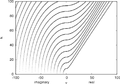
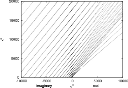
(a) (b)

Figure 2: Two different representations of mode numbers $\nu$ at the corresponding wavenumbers $k$ in the bend with $q=0.6$. In (a) we plot $k$ vs. $\nu$, where we separately discuss real and imaginary mode numbers depicted on the right and left side of the abscissa, respectively, and in (b) we plot $k^{2}$ vs. $\nu^{2}$. The dashed lines represent solutions of equation (26).

The highest real mode $\nu_{\rm max}$ for small wave-numbers $k<\nu$ can be approximated using equation (25) as

$$\nu_{\rm max}(k,q)\approx\frac{\pi}{|\log q|}\sqrt{\left(\frac{k}{k_{0}(1,q)}\right)^{2}-1}\>.$$ (27)

In practical applications it is important that below the wave-number $k_{\rm low}(q)=k_{0}(1,q)$ there are no real modes. In wide bends with $q\approx 0$ one can expand the cross-product of Bessel functions around $q=0$ and obtain the formula

$$k_{\rm low}(q)=b_{0}+\frac{b_{1}}{|\log q|}+O(q^{2})\>,$$ (28)

where $b_{0}$ is the smallest zero of the Bessel function $J_{0}(x)$, $J_{0}(b_{0})=0$ and

$$b_{0}\doteq 2.404825558\>,\qquad b_{1}=-\frac{\pi Y_{0}(b_{0})}{2J^{\prime}_{0}(b_{0})}\doteq 1.54288974\>.$$ (29)

In narrow bends, where $a(=1-q)\to 0$, we can use standard stationary perturbation theory [21], see equation (118) in B, to approximate $k_{\rm low}(q)$. By introducing the matrix elements

$$V_{nm}=-\frac{1}{2}\int_{0}^{1}{\rm d}x\,\frac{\sin(\pi nx)\sin(\pi mx)}{(x+\gamma)^{2}}\>,\quad\gamma=\frac{q}{1-q}\>,$$ (30)

we can express the lowest wave-number as

$$k_{\rm low}(q)=\frac{\pi}{a}\left[1+\frac{1}{\pi^{2}}V_{11}+\frac{1}{\pi^{4}}\sum_{l>1}\frac{|V_{1l}|^{2}}{1-l^{2}}+O\left(|V|^{3}\right)\right]^{1/2}\>.$$ (31)

The formula (31) has a simple first order expansion in $a=1-q$

$$k_{\rm low}(q)=\frac{\pi}{a}-\frac{a}{8\pi}+O\left(a^{2}\right)\>.$$ (32)

From the expression (32) we learn that the lowest wave-number at which real modes exists increases with increasing $q$ and converges to $\frac{\pi}{a}$.

2.2 Numerical evaluation of mode functions in a bend

The mode functions in the bend at a given wave-number $k$ and inner radius $q$ are proportional to cross products of Bessel functions $Z_{\nu,k}(r)$ (12), where the order parameter $\nu$ takes values from the set ${\cal M}_{k,q}$. Because of the symmetry $Z_{-\nu,k}(r)=Z_{\nu,k}(r)$, we only consider mode numbers from the set ${\cal M}_{k,q,+}=\{\nu_{n}:\nu_{n}^{2}>\nu_{n+1}^{2}\>,\;n\in{\mathbb{N}}\}$, which are ordered by decreasing square. To illustrate the basic properties of mode functions, we plot in figure 3 the functions $Z_{\nu,k}(r)$ for real and first few imaginary mode numbers for $q=0.6$ and some low wave-number $k$. We see that the first mode function $Z_{\nu_{1},k}(r)$ has no zeroes on the interval $r\in(q,1)$ and each consecutive mode function has one additional zero. In the following, we present formulae and numerical recipes for stable calculation of mode functions, where we assume that the mode numbers are given.

Figure 3: Plots of $Z_{\nu_{n},k}(r)$ for first 12 mode-numbers $\nu_{n}\in{\cal M}_{k,q,+}$ $(\nu_{n}^{2}>\nu_{n+1}^{2})$ calculated at the wave-number $k=78.5398$ $(N_{\rm b}=10)$ and inner radius $q=0.6$.

The Bessel functions for real orders are well implemented in the currently available numerical libraries, i.e. SLATEC [22]. From the definitions of Bessel functions it is not unexpected that we encounter problems at evaluating $Z_{\nu,k}$ for large wavenumbers $k\gg 1$ and high real orders $\nu\gg 1$. In order to overcome these problems we apply the stable forward recursions in the order parameter [19] written as

$$\hskip 28.45274ptp_{\mu+1} = p_{\mu-1}-2\mu(xq_{\mu}+yr_{\mu})\>,$$ (33)

$$\hskip 28.45274ptq_{\mu+1} = (2\mu(\mu+1)y^{2}-1)r_{\mu}+2\mu(\mu+1)xyq_{\mu}-(\mu+1)yp_{\mu-1}+\mu xp_{\mu}\>,$$ (34)

$$\hskip 28.45274ptr_{\mu+1} = (2\mu(\mu+1)x^{2}-1)q_{\mu}+2\mu(\mu+1)xyr_{\mu}-(\mu+1)xp_{\mu-1}+\mu yp_{\mu}\>,$$ (35)

where we write $x=(kr)^{-1}$ and $y=k^{-1}$ and define the following symbols

$$p_{\mu} = J_{\mu}(kr)Y_{\mu}(k)-J_{\mu}(k)Y_{\mu}(kr)\>,$$ (36)

$$q_{\mu} = J_{\mu}(kr)Y^{\prime}_{\mu}(k)-J^{\prime}_{\mu}(k)Y_{\mu}(kr)\>,$$ (37)

$$r_{\mu} = J^{\prime}_{\mu}(kr)Y_{\mu}(k)-J_{\mu}(k)Y^{\prime}_{\mu}(kr)\>.$$ (38)

The initial conditions for the recursion, at low orders, are calculated using standard routines and the expressions for the derivatives of Bessel functions, e.g. a relation valid for any Cylindrical function: $C^{\prime}_{\nu}=(C_{\nu-1}-C_{\nu+1})/\nu$. However, we encountered a problem at high wavenumbers and low orders due to the lack of precision in SLATEC routines. Therefore in that regime we use the Hankel approximation [19] to evaluate $Z_{\nu,k}$

$$\hskip 28.45274ptZ_{\nu,k}(r)=\frac{2}{\pi\sqrt{r}k}\left[(AC+BD)\sin(k(1-r))+(AD-BC)\cos(k(1-r))\right]\>,$$ (39)

where we write $A=P_{\nu}(kr)$, $B=Q_{\nu}(kr)$, $C=P_{\nu}(k)$ and $D=Q_{\nu}(k)$, which are expressed in terms of the asymptotic series:

$$\hskip 28.45274ptP_{\nu}(z)=1-\frac{(\mu-1)(\mu-9)}{2!(8z)^{2}}+\frac{(\mu-1)(\mu-9)(\mu-25)(\mu-49)}{4!(8z)^{4}}+\ldots$$ (40)

and

$$\hskip 28.45274ptQ_{\nu}(z)=\frac{\mu-1}{8z}-\frac{(\mu-1)(\mu-9)(\mu-25)}{3!(8z)^{3}}+\ldots\>,\qquad\mu=4\nu^{2}\>,$$ (41)

which we sum up to $l_{\rm max}=\lfloor\nu/2\rfloor+1$ terms. There is another difficulty occurring at high wave-numbers, which can not be corrected. The first few real modes $\nu_{p}\in{\cal M}_{k,q,+}$ scale linearly with the wavenumber $k$ and functions $Z_{\nu,k}(r)$ diverge with increasing order $\nu$. Consequently, the values $Z_{\nu,k}(q)$ are exponentially sensitive on the precision of the first few mode numbers $\nu_{p}$:

$$|Z_{\nu_{p}+\delta\nu,k}|(q)\sim q^{-|\nu_{p}|}\sinh(|\log q|\,\delta\nu)\>.$$ (42)

This problem can not be solved completely, but only partially corrected by manually setting the values of $Z_{\nu_{p},k}(r)$ to zero around the inner radius. This can be done without any real loss of precision, because the mode functions are localised near outer radius. In practice we calculate the left side of equation (42) in a finite range arithmetic $[-m,m]$ with the maximal number $m$ (e.g. $m\approx 10^{308}$ in double precision). By considering that together with the known property $\nu_{\rm max}\sim k$ (23), we find that in practice our modal approach breaks down above some wave-number $k_{\rm break}\sim\log m/|\log q|$ and consequently bounding the number of open modes in our numerical analysis below

$$N_{\mathrm{o,{\rm break}}}\sim\frac{a}{\pi}\frac{\log m}{|\log q|}\>,$$ (43)

where we used the relation $N_{\rm o}\sim ka/\pi$ valid for narrow bends and high wave-numbers.

The numerical evaluation of $Z_{\nu_{p},k}(r)$ at imaginary orders $\nu\in{\rm i}{\mathbb{R}}$ is almost unsupported in currently available numerical libraries. Therefore we have developed procedures for their evaluation ourselves and give here a summary of our work. For each regime of order parameters $\nu={\rm i}y$ and wavenumbers $k$ we use a different strategy to evaluate $Z_{{\rm i}y,k}(r)$ in order to achieve an optimal precision control and a CPU time consumption. The formula for the cross-products of Bessel functions (12) takes for imaginary orders a simple form

$$Z_{{\rm i}y,k}(r)=\frac{2}{\sinh(\pi y)}\Im\left\{J_{{\rm i}y}(k)J_{{\rm i}y}^{*}(kr)\right\}\>.$$ (44)

At small wave-numbers $k$ or more generally for $k\ll y$, we use the Taylor expansion of the Bessel function [19] and rewrite equation (44) into

$$Z_{{\rm i}y,k}(r)=\frac{2}{\pi y}\Im\left\{r^{-{\rm i}y}u_{{\rm i}y}(k)u_{{\rm i}y}^{*}(kr)\right\}\>,$$ (45)

where we use the series

$$u_{\nu}(z)=\sum_{l=0}^{\infty}\frac{(-1)^{l}\left(\frac{z}{2}\right)^{2l}}{l!\,(\nu+1,\nu+l+1)}\>,\qquad(x,y)=\frac{\Gamma(y)}{\Gamma(x)}\>.$$ (46)

The series (46) is summed up to the index $l_{\rm max}=\lfloor\sqrt{z^{2}/\epsilon+|\nu|^{2}/4}\rfloor$, where $\epsilon$ is the desired accuracy of the expression.

At higher wave-numbers $k$ and orders $y\lesssim k$ we combine the backwards recursion valid for Cylindrical functions

$$a_{l-1}(z)=\frac{2(l+{\rm i}y)}{z}a_{l}(z)-a_{l+1}(z)\>,$$ (47)

with an appropriate normalisation formula for $a_{l}(z)$ [19] and thereby obtain an expression for $u_{{\rm i}y}(k)$ (45) given by

$$u_{{\rm i}y}(z)=a_{0}(z)\left[\sum_{l=0}^{\infty}\frac{(2l+z)(1+z,l+z)}{l!}a_{2l}(z)\right]^{-1}\>.$$ (48)

The terms $a_{2l}$ in the series (48) are given with the recursion (47) started at the index $l_{\rm max}=2\lfloor(x+1)/2\rfloor$ with initial conditions $a_{l_{\rm max}}=\varepsilon$ and $a_{l_{\rm max}+1}=0$, where constant $\varepsilon$ is the smallest number supported by the CPU architecture and $x$ is determined by the equation

$$|\log\varepsilon|-1+\frac{1}{2}\log(1+y^{2})-y\operatorname{arctan}\,y=$$

$$\frac{1}{2}x\log(x^{2}+y^{2})-x\left(\log\frac{z}{2}+1\right)-x\operatorname{arctan}\frac{y}{x}\>.$$ (49)

The later equation (49) is meaningful only if the right side is positive, yielding that presented approach with the iteration formula is valid only for orders $y$ below some value scaling as $O(|\log\varepsilon|)$. By increasing the wavenumber $k$ further up and keeping orders small $y\ll k$ we can use the Hankel approximation (39) with the order parameter $\nu={\rm i}y$. The asymptotic series (40) and (41) in the expression (39) are summed at least up to $l_{\rm max}=\lfloor z/2+\sqrt{2z^{2}-y^{2}/2}\rfloor$ terms. At large enough wavenumbers $k$ and imaginary orders $y>k$ we can make use of the Debye approximation of Bessel functions [23] and write

$$Z_{{\rm i}y}(k,r)=\frac{2}{\pi}\frac{\Im\left\{G(\alpha,\xi)G^{*}(\beta,\zeta)e^{{\rm i}\left[\xi-\zeta-y\left(\operatorname{arcsinh}\frac{y}{k}-\operatorname{arcsinh}\frac{y}{kr}\right)\right]}\right\}}{(1-e^{-2\pi y})\sqrt{\xi\zeta}}\>,$$ (50)

with substitutions

$$\hskip 28.45274pt\xi=\sqrt{y^{2}+k^{2}}\>,\quad\zeta=\sqrt{y^{2}+(kr)^{2}}\>,\quad\alpha^{-1}=1+\frac{k^{2}}{y^{2}}\>,\quad\beta^{-1}=1+\frac{(kr)^{2}}{y^{2}}\>.$$ (51)

The expression $G(x,y)$ in formula (50) is given in the form of an asymptotic series

$$G(x,y)=\sum_{m=0}^{\infty}\frac{(-{\rm i})^{m}v_{m}(x)}{y^{m}}\>,$$ (52)

where polynomials $v_{m}(t)$ are generated by the following recursion

$$\hskip 28.45274ptv_{k+1}(t)=\frac{1}{2}(1-t)\left(k\,v_{k}(t)+2t\,{v^{\prime}}_{k}(t)\right)+\frac{1}{16}t^{-\frac{k+1}{2}}\int_{0}^{t}(1-5\tau)\tau^{\frac{k-1}{2}}v_{k}(\tau)\,{\rm d}\tau\>.$$ (53)

The first few $v_{m}(t)$ read as

$$\hskip 28.45274ptv_{0}(t)=1,\quad v_{1}(t)=\frac{1}{8}-\frac{5}{24}t,\quad v_{2}(t)=\frac{3}{128}-\frac{77}{576}t+\frac{385}{3456}t^{2}\>,\ldots\>.$$ (54)

The formulae (39, 45, 48, 50) enable a stable high precision calculation of the mode functions in the bend at imaginary mode numbers.

2.3 The overlap of mode-functions in different geometries

The main ingredient in the modal description of the scattering are the overlap integrals of mode functions in the straight waveguide and in the bend. These overlap integrals “tell” about the compatibility of both scattering regions and are discussed in the following.

The cross products of Bessel functions with order parameter $\nu\in{\cal M}_{k,q,+}$ at given wavenumber $k$ and inner radius $q$ form a set of functions

$${\cal Z}_{k,q}=\{Z_{\nu,k}(r):\nu\in{\cal M}_{k,q,+},r\in[q,1]\}\>,$$ (55)

which is complete in $L_{2}[q,1]$ and orthogonal w.r.t. the weight function $w(r)=r^{-1}$. The later is derived in A. The orthogonality relation for $Z_{\nu,k}\in{\cal Z}_{k,q}$ reads [24]

$$\hskip 14.22636pt\int_{q}^{1}{\rm d}r\,w(r)Z_{\nu,k}(r)Z_{\mu,k}(r)=\delta_{\mu,\nu}\frac{k}{2\nu}\left[Z_{\nu+1,k}(1)\frac{\partial Z_{\nu,k}}{\partial\nu}(1)-qZ_{\nu+1,k}(q)\frac{\partial Z_{\nu,k}}{\partial\nu}(q)\right]\>.$$ (56)

The line separating the bend and the straight wave-guide will be called the cross-section of our open-billiard. On the cross-section we define two different scalar products denoted by $(\cdot,\cdot)$ and $\left\langle\cdot,\cdot\right\rangle$, and written as

$$(a,b)=\int_{q}^{1}\frac{{\rm d}r}{r}a(r)\,b(r)\>,\qquad\left\langle a,b\right\rangle=\int_{0}^{a}{\rm d}y\,a(y)\,b(y)\>.$$ (57)

Let us now introduce modes at some fixed wave-number $k$ and inner radius $q$ for different regions of the open billiard. In the bend, mode numbers $\nu_{p}$ and normalised mode functions $U_{p}(r)$ read as

$$\nu_{p}\in{\cal M}_{k,q,+}\>,\quad U_{p}(r)=\frac{Z_{\nu_{p},k}(r)}{\sqrt{(Z_{\nu_{p},k},Z_{\nu_{p},k})}}\>,\qquad p\in{\mathbb{N}}\>,$$ (58)

where we order the mode numbers so that $\nu^{2}_{p}>\nu_{p+1}^{2}$, and in the straight leads connected to the bend we have mode numbers $g_{n}$ and mode functions $u_{n}(x)$ defined by

$$g_{n}=\sqrt{k^{2}-\left(\frac{\pi n}{a}\right)^{2}}\>,\quad u_{n}(y)=\sqrt{\frac{2}{a}}\sin\left(\frac{\pi}{a}ny\right)\>,\qquad n\in{\mathbb{N}}\>.$$ (59)

The modes with real and imaginary mode numbers are called open and closed modes, respectively. The number of open modes in some geometry is denoted by $N_{\rm o}$. The overlap integrals of mode functions are given by

$$A_{np}=\left\langle u_{n},U_{p}\right\rangle\>,\qquad B_{np}=(u_{n},U_{p})\>,$$ (60)

where we use the relation $r=q+y$ between the coordinates. In figure 4 we show a density plot of the matrix elements, in log scale, namely $\log|A_{np}|$ and $\log|B_{np}|$, at two values of inner radii with the same number of open modes $N_{\rm o}$ in both geometries.

$q=0.2$                                  $q=0.9$

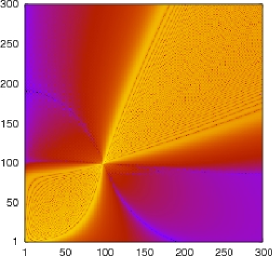
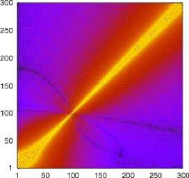
$\log_{10}|A_{np}|$

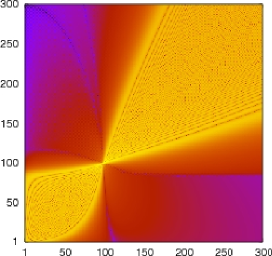
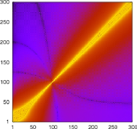
$\log_{10}|B_{np}|$

                             

Figure 4: Density plots of the matrix elements $\log_{10}|A_{np}|$ (top-row) and $\log_{10}|B_{np}|$ (bottom-row) for $q=0.2$ (left) and $q=0.9$ (right) as indicated in the figure. The number of open modes is $N_{\rm o}=100$ and the number of all considered modes is $N=300$.

We see that the matrices $A_{np}$ and $B_{np}$ have a similar form for all $q$ and $k$. This is starting at small indices with a wide area of high values of matrix elements that squeezes to almost a single intensified point at $n,p\approx N_{\rm o}$ again spreading in a triangular shape with increasing indices. The parameter $q$ has a strong influence on the shape of the area with high intensities in $A$ and $B$. In the case of small values of $q$ in contrast to larger $q$, the area of high values in matrices $A$ and $B$ covers almost the whole open-open block of indices and with crossing of the narrowing at $n,p\approx N_{\rm o}$ spreads faster with increasing indices. The shape of matrices $A$ and $B$ is similar therefore in the following we only show results for the matrix $A_{np}$. We found numerically that the area of high intensities in matrices $A$ and $B$ scales with the number of open modes $N_{\rm o}$ as $A_{np},B_{np}\sim F(n/N_{\rm o},p/N_{\rm o})$, where $F$ is some a well behaved function. We demonstrate this by plotting the matrix elements $|A_{np}|$ in relative indices $n/N_{\rm o}$ and $p/N_{\rm o}$ for different numbers of open modes $N_{\rm o}$ shown in figure 5.

$N_{\rm o}=100$ $N_{\rm o}=200$ $N_{\rm o}=400$

                              

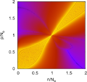
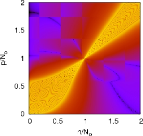
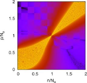
Figure 5: Density plot of matrix elements $\log_{10}|A_{np}|$ at inner radius $q=0.6$ and different number of open modes $N_{\rm o}=$ 100, 200, and 400 as indicated in the figure.

In addition, we find numerical evidence that intensities of matrix elements $A_{np}$ and $B_{np}$ in the region of open modes and in the region of closed modes scale differently with $N_{\rm o}$

open modes $$: |A_{np}|,\;|B_{np}|\lesssim\frac{1}{\sqrt{N_{\rm o}}}F_{\rm max}\left(\frac{n}{N_{\rm o}},\frac{p}{N_{\rm o}}\right)\>,$$ (61)

closed modes $$: |A_{np}|,\;|B_{np}|\lesssim\frac{1}{N_{\rm o}^{2}}F_{\rm min}\left(\frac{n}{N_{\rm o}},\frac{p}{N_{\rm o}}\right)\>.$$ (62)

where $F_{\rm max}$ and $F_{\rm tail}$ are some well behaved functions. Taking into account these phenomenological findings enables a better precision control of scattering calculations. In figure 6 we see that $F_{\rm max}$ is an envelope function for maximal values of $N_{\rm o}^{1\over 2}|A_{np}|$ and that $F_{\rm min}$ can be chosen to fit the tails of $N_{\rm o}^{2}|A_{np}|$.

Figure 6: The cuts in the index space of matrix $A_{np}$ at fixed $p/N_{\rm o}=0.5$ and different number of open modes $N_{\rm o}=$ 50, 100, 200, and 400 at inner radius $q=0.6$.

We prove the scaling relation (62) by using an asymptotic approximation of the mode function in the bend

$$U_{p}(r)=\sqrt{\frac{2}{|\log q|}}\sin\left(\frac{\pi p}{\log q}\log r\right)\>,\quad p\gg 1\>,$$ (63)

which yields the following asymptotic behaviour of matrix elements

$$A_{np}\approx\frac{6}{\pi^{2}}\frac{|\log q|^{5\over 2}}{(1-q)^{3\over 2}}\left(q^{2}(-1)^{p}+(-1)^{n+1}\right)np^{-3}+O(p^{-5})\quad n=\textrm{fixed},\;p\to\infty\>,$$ (64)

$$A_{np}\approx\frac{2}{\pi^{2}}\frac{(1-q)^{5\over 2}}{|\log q|^{3\over 2}}\left(q^{-2}(-1)^{p+1}+(-1)^{n}\right)pn^{-3}+O(n^{-5})\quad p=\textrm{fixed}\gg 1,\;n\to\infty\>.$$ (65)

The off-diagonal diagonal elements $A_{np}$ and $B_{np}$ decay algebraically with increasing index. The pre-factor of the decay is decreasing with increasing $q$ and is singular at $q=0$. This means that for large enough $q$ it is possible to approximately express the open modes of the bend solely in terms of open modes of the straight waveguide and vice versa, as indicated by the relation (61).

From the definition of matrix elements $A_{np}$ and $B_{np}$ (60), and completeness of the mode functions at given $k$ and $q$, it follows that $A$ and $B$ are transition matrices between the sets of mode functions in different regions,

$$u_{n}(x)=\sum_{p\in{\mathbb{N}}}B_{np}\,U_{p}(r)\>,\qquad U_{p}(r)=\sum_{n\in{\mathbb{N}}}A_{np}\,u_{n}(x)\>,$$ (66)

yielding the relation

$$AB^{T}=A^{T}B={\rm id}\>.$$ (67)

In practice we work with finite sets of modes, where the identity (67) cannot hold exactly.

                        $q=0.2$                                $q=0.6$                                $q=0.9$

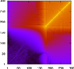
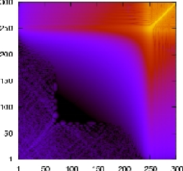
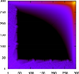
Figure 7: Density plot of matrix elements $\log_{10}|(AB^{T})_{nm}-\delta_{nm}|$ for $q$ = 0.2, 0.6 and 0.9 (from left to right). On the abscissa and ordinate we plot indices $n$ and $m$, respectively. The number of open modes is $N_{\rm o}=100$ and the total number of modes is 300.

In figure 7 we plot $AB^{T}$ for different inner radii $q$ and fixed $N_{\rm o}=100$. The mismatch from the identity (67) on some sub-set of indices starting at the origin $n=1$, or $p=1$, increases with decreasing inner radius $q$. This means that the numerical calculation of scattering for smaller $q$ should be less accurate at finite dimensions. The discrepancy between $AB^{T}$ and the identity on (truncated) finite dimensional spaces is strongly non-uniform in indices. Before going into practical aspects of this problem, we examine the convergence of matrix elements $(AB^{T})_{nm}$ to $\delta_{nm}$ with increasing number of all considered modes $N=N_{\rm o}+N_{\rm c}$ at fixed $N_{\rm o}$, where $N_{\rm c}$ is the number of closed modes. An example of such convergence is shown in figure 8.

                        $N_{\rm c}=1$                                 $N_{\rm c}=100$                                $N_{\rm c}=500$              

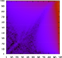
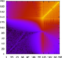
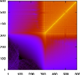
Figure 8: Density plot of matrix elements $\log_{10}|(AB^{T})_{nm}-\delta_{nm}|$ for different numbers of closed modes $N_{\rm c}$ = 1, 100 and 500, as indicated in the figure, at inner radius $q=0.2$ and $N_{\rm o}=100$ open modes. The labels on the abscissa and the ordinate are matrix indices $n$ and $m$, respectively.

The convergence proceeds by the standard scenario, where the agreement between $[AB^{T}]_{np}$ and $\delta_{np}$ propagates block-wise from low to higher indices with increasing $N$. The propagation is slow due to the triangular shaped area of high intensities in the closed-closed modes block of $A$ and $B$. The speed of propagation of accuracy to higher indices increases with increasing inner radius $q$.

The SVD decompositions [25] of matrices $A$ and $B$ is useful for improving and stabilising the scattering calculations and will be used in the next section. From definitions of transition matrices (60) and completeness of mode functions we obtain

$$(AA^{T})_{nn^{\prime}} =\left\langle u_{n},r\,u_{n^{\prime}}\right\rangle\>,\qquad(A^{T}A)_{pp^{\prime}} =(U_{p},r\,U_{p^{\prime}})\>,$$ (68)

$$(BB^{T})_{nn^{\prime}} =\left\langle u_{n},r^{-1}\,u_{n^{\prime}}\right\rangle\>,\qquad(B^{T}B)_{pp^{\prime}} =(U_{p},r^{-1}\,U_{p^{\prime}})\>.$$ (69)

which we use to bound the image

$$\frac{\|Aa\|_{2}}{\|a\|_{2}}\in[q^{1\over 2},1]\>,\quad\frac{\|Ba\|_{2}}{\|a\|_{2}}\in\left[1,q^{-{1\over 2}}\right]\quad\textrm{for}\quad\|a\|_{2}\neq 0\>.$$ (70)

These results together with $AB^{T}={\rm id}$ can be used to determine the form of the SVD decomposition

$$A=U\Sigma V^{T}\>,\quad B=U\Sigma^{-1}V^{T}\>,\quad\Sigma=\operatorname{diag}\left\{\sigma_{i}\in[\sqrt{q},1]\right\}_{i\in{\mathbb{N}}}\>,$$ (71)

where $U$ and $V$ are orthogonal matrices. We show here an example of the SVD decomposition of finite dimensional matrices $A$ and $B$ at $q=0.2$ and $N_{\rm o}=100$. In figure 9 we show singular values and in figure 10 we show density plots of the corresponding matrices $U$ and $V$, where the inner indices are ordered by decreasing magnitude of singular values.

Figure 9: Singular values of matrices $A$ (left) and $B$ (right) for different number of closed modes $N_{\rm c}$ = 100, 200, 300, 400 and 500 at $q$ =0.2 and $N_{\rm o}$ = 100.

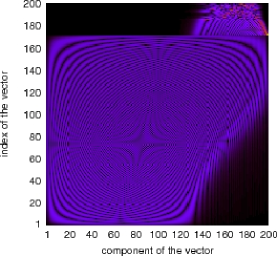
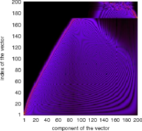
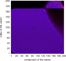
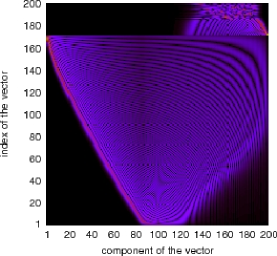
Figure 10: Density plots of matrix elements $|U_{nm}|$ (left) and $|V_{nm}|$ (right) of the SVD decomposition of matrices $A$ (top row) and $B$ (bottom row) at inner radius $q=0.2$ with $N_{\rm o}=100$ open and $N_{\rm c}=100$ closed modes. Labels on the abscissa and the ordinate are indices $n$ and $m$, respectively.

We see that the relative dimension of the space, which violates the bounds of the singular spectra (70), converges with increasing space dimension $N=N_{\rm o}+N_{\rm c}$, where $N_{\rm c}$ is the number of imaginary modes. In the presented case $q=0.2$ the relative dimension is around $20\%$. It is important to see that vectors in $V$ and $U$ corresponding to singular values, which violate the bounds, have non-zero components only at closed modes. We conclude that due to a finite dimensional representation of matrices $A$ and $B$ we have deviations from the infinitely dimensional case only at high laying decaying modes that span a space of almost fixed relative dimension for some value of $q$.

3 The scattering across a bend

In this section we solve the on-shell scattering of a non-relativistic particle across our open billiard using the modal approach, initiated in the introduction. The scattering is discussed at fixed wave-number $k$ and inner radius $q$. The control of the precision of scattering calculations is studied in detail. In the second part of this section we investigate some interesting physical scattering properties of the bend.

3.1 The scattering matrix of a bend

The scattering matrix $S$ [18] is a linear mapping between the incoming and outgoing “waves” with respect to our scatterer. We reorganise the expansion coefficients of the wave function over different regions (9), (10), (11) into the incoming contributions denoted as $v_{\rm in}=(a^{+}_{1},a^{+}_{2},\ldots,b^{-}_{1},b^{-}_{2},\ldots)$ and outgoing contributions $v_{\rm out}=(a^{-}_{1},a^{-}_{2},\ldots,b^{+}_{1},b^{+}_{2},\ldots)$. Then the scattering matrix $S$ can be defined as

$$Sv_{\rm in}=v_{\rm out}\>.$$ (72)

The S-matrix in our case has a simple symmetric block form

$$S={\left[\begin{array}[]{cc}R&T\cr T&R\end{array}\right]}\>,$$ (73)

with $R$ and $T$ being the reflection and the transmission matrix, respectively. By reordering of rows and columns in $S$ so that the matrix elements concerning open (subscript $\rm o$) and closed (subscript $\rm c$) modes are separated and grouped together we obtain the matrix ${\cal S}$, reading

$$S\to{\cal S}={\left[\begin{array}[]{cc}{\cal S}_{\rm oo}&{\cal S}_{\rm oc}\cr{\cal S}_{\rm co}&{\cal S}_{\rm cc}\end{array}\right]}\>.$$ (74)

We find that blocks of matrix ${\cal S}$ (74) obey the generalised unitarity [26] defined by the following relations

$${\cal S}_{\rm oo}{\cal S}_{\rm oo}^{\dagger} = {\cal S}_{\rm oo}^{\dagger}{\cal S}_{\rm oo}={\rm id}\>,$$ (75)

$${\rm i}\,{\cal S}_{\rm oo}{\cal S}_{\rm co}^{\dagger} = {\cal S}_{\rm oc}\>,$$ (76)

$${\rm i}\,{\cal S}_{\rm oc}^{\dagger}{\cal S}_{\rm oo} = {\cal S}_{\rm co}\>,$$ (77)

$${\rm i}\,{\cal S}_{\rm co}{\cal S}_{\rm co}^{\dagger} = {\rm i}\,{\cal S}_{\rm oc}^{\dagger}{\cal S}_{\rm oc}={\cal S}_{\rm cc}-{\cal S}^{\dagger}_{\rm cc}\>.$$ (78)

The relations (75 - 78) result from the probability current conservation, which is also equivalent to the condition $AB^{T}={\rm id}$. Due to the time-reversal symmetry of the physical problem the scattering matrices $S$ and ${\cal S}$ are symmetric

$$S^{T}=S\>,\qquad{\cal S}^{T}={\cal S}\>.$$ (79)

The block symmetry of the scattering matrix (73) simplifies its calculation. We may consider individual incoming waves $e_{n}^{+}$ represented by the following wave function ansatz

$$\psi({\bf r}) =e^{+}_{n}({\bf r})+\sum_{m}e^{-}_{m}({\bf r})\;R_{mn}\>,\qquad {\bf r}\in\Omega_{\rm A}\>,$$ (80)

$$\psi({\bf r}) =\sum_{p}f^{+}_{p}({\bf r})\;\Lambda^{+}_{pn}+f^{-}_{p}({\bf r})\;\Lambda^{-}_{pn}\>,\qquad {\bf r}\in\Omega_{\rm B}\>,$$ (81)

$$\psi({\bf r}) =\sum_{m}e^{+}_{m}({\bf r})\;T_{mn}\>.\qquad {\bf r}\in\Omega_{\rm C}\>,$$ (82)

The continuity of $\psi({\bf r})$ and its normal derivative on the connecting cross-sections between regions $\Omega_{\rm A,B,C}$ determines the matrix elements $R_{mn}$, $T_{mn}$ and $\Lambda^{\pm}_{pn}$ and yields the following system of matrix equations

$${\rm id}+R=M(\Lambda^{+}+\Lambda^{-})\>,\qquad T=M({\cal F}\Lambda^{+}+{\cal F}^{-1}\Lambda^{-})\>,$$ (83)

$${\rm id}-R=N(\Lambda^{+}-\Lambda^{-})\>,\qquad T=N({\cal F}\Lambda^{+}-{\cal F}^{-1}\Lambda^{-})\>,$$ (84)

$$M=G^{\frac{1}{2}}AV^{-\frac{1}{2}}\>,\qquad N=G^{-\frac{1}{2}}BV^{\frac{1}{2}}\>,$$ (85)

which we write using diagonal matrices $V=\operatorname{diag}\{\nu_{n}\}_{n\in{\mathbb{N}}}$, $G=\operatorname{diag}\{g_{n}\}_{n\in{\mathbb{N}}}$ and ${\cal F}=\exp({\rm i}V)$, and transition matrices $A$ and $B$ (60). The elimination of matrices $\Lambda^{\pm}$ from equations (83) and (84) yields the blocks of the scattering matrix $S$, reading

$$T=(C-{\cal F}DC^{-1}{\cal F}D)^{-1}{\cal F}(C-DC^{-1}D)\>,$$ (86)

$$R=(C-{\cal F}DC^{-1}{\cal F}D)^{-1}({\cal F}DC^{-1}{\cal F}C-D)\>,$$ (87)

that we express by using the following auxiliary matrices

$$C=M^{-1}+N^{-1}=V^{1\over 2}B^{T}G^{-{1\over 2}}+V^{-{1\over 2}}A^{T}G^{1\over 2}\>,$$ (88)

$$D=M^{-1}-N^{-1}=V^{1\over 2}B^{T}G^{-{1\over 2}}-V^{-{1\over 2}}A^{T}G^{1\over 2}\>,$$ (89)

where we take into account the relation $AB^{T}={\rm id}$. The presented form of the matrix $T$ (86) and $R$ (87) is chosen in order to increase its numerical stability i.e. minimising the use of inverses and avoiding direct computation of ${\cal F}^{-1}$.

3.2 Numerically stable scheme for scattering matrix calculation

A bend on a straight waveguide is a paradigmatic example for testing numerical schemes and ideas on how to accurately calculate the scattering matrix. In particular, the high curvature case $q\to 0$ turns to be highly non-trivial. Here we give a simple and stable procedure to obtain the scattering matrix with a clear precision control for practically all curvatures.

The scattering across a bend of angle $\beta$ and inner radius $q$ back to asymptotic region at some wavenumber $k$ is described by the scattering matrix $S(\beta)$ (73), which is composed of the reflection matrix $R(\beta)$ (87) and the transmission matrix $T(\beta)$ (86). In practice, we work with finite dimensional matrix approximations, denoted by

$$R_{N}(\beta),\;T_{N}(\beta)\in{\mathbb{C}}^{N\times N}\>,\quad S_{N}(\beta)\in{\mathbb{C}}^{2N\times 2N}\>,\quad A_{N},B_{N}\in{\mathbb{R}}^{N\times N}\>.$$ (90)

where $N\geq N_{\rm o}$ is the number of modes used in the asymptotic regions. The main objective is to construct these finite dimensional matrices $R_{N}(\beta)$ and $T_{N}(\beta)$ so that:

1. calculations are numerically stable and precise,

2. $S_{N}(\beta)$ satisfies the time reversal symmetry (79) and the generalised unitarity relation (75 - 77),

3. the sub-block of $R_{N}(\beta)$ and $T_{N}(\beta)$ of dimension $N^{\prime}\in(N_{\rm o},N]$ is calculated with controllable accuracy, where $N_{\rm o}=\lfloor ka/\pi\rfloor$ is the number of open modes in the asymptotic region.

The recipe to achieve these assumptions may be separated into two parts. In the first part we cure the numerical instability caused by the maximal element $r(\beta)=\exp(\beta\nu_{N})$ in ${\cal F}_{N}(\beta)$, which are exponentially diverging with increasing $N$. This is achieved by separating the bend into $2^{n_{0}}$ identical subsections of angle $\beta^{\prime}=2^{-n_{0}}\beta$ so that $r(\beta^{\prime})\varepsilon_{\rm num}\approx 1$, where $\varepsilon_{\rm num}$ is the numerical precision e.g. $\varepsilon_{\rm num}=2^{-52}$ in double precision floating point arithmetic. The number $n_{0}$ is calculated as

$$n_{0}=\max\left\{0,\;1+\left\lfloor\log_{2}\left(\frac{|\log\varepsilon_{\rm num}|}{\beta\nu_{N}}\right)\right\rfloor\right\}\>.$$ (91)

The scattering matrix $S_{N}(\beta^{\prime})$ of a small subsection of the bend can be calculated in a very stable way and up to a high precision. By concatenating scattering matrices of subsections together with the recursion

$$S_{N}(2^{-m+1}\beta)=S_{N}(2^{-m}\beta)\odot S_{N}(2^{-m}\beta)\>.$$ (92)

we obtain the scattering matrix of the whole bend $S_{N}(\beta)$. The symbol $\odot$ denotes the operation for concatenating scattering matrices associated to scatterers on the waveguide and is defined in C.

In the second part we are discussing the problem that $S_{N}(\beta^{\prime})$ diverges with increasing $N$, which is due to violation of the identity $AB^{T}={\rm id}$ (67) for finite truncated transition matrices $A_{N}$ and $B_{N}$. We eliminate the problem by deforming $A_{N}$ and $B_{N}$ so that they are non-singular and exactly fulfil the condition $A_{N}B_{N}^{T}={\rm id}$. We make the SVD decomposition of the truncated matrix $A_{N}=U_{N}\Sigma_{N}V^{T}_{N}$, modify its singular values $\Sigma_{N}=\operatorname{diag}\{\sigma_{i}\}_{i=1}^{N}$ to $\tilde{\Sigma}_{N}=\operatorname{diag}\{\tilde{\sigma}_{i}\}_{i=1}^{N}$ so that they fit in the bounds obtained for infinitely dimensional case (71)

$$\tilde{\sigma}_{i}=\left\{\begin{array}[]{lll}\sigma_{i}&:&\sigma_{i}\in[q^{1\over 2},1]\cr\sigma^{*}&:&{\rm otherwise}\end{array}\right.\>,$$ (93)

and again generate both matrices

$$\widetilde{A}_{N}=U_{N}\widetilde{\Sigma}_{N}V^{T}_{N}\>,\qquad\widetilde{B}_{N}=U_{N}\widetilde{\Sigma}_{N}^{-1}V^{T}_{N}\>.$$ (94)

The same procedure can also be done using SVD decomposition of the matrix $B_{N}$ as a base for generation of both deformed matrices $\widetilde{A}_{N}$ and $\widetilde{B}_{N}$. The value of $\sigma^{*}>0$ can be chosen arbitrarily, but the most elegant choice is $\sigma^{*}=1$. By using matrices $\widetilde{A}_{N}$ and $\widetilde{B}_{N}$ (94) instead of $A_{N}$ and $B_{N}$ in $S_{N}(\beta^{\prime})$ and consequently in $S_{N}(\beta)$ these become generalised unitary with a well behaved and physically precise limit $N\to\infty$ at least on the sub-space of dimension $N^{\prime}$. We first check this by discussing the precision of transition between the modes in the bend and in the straight waveguide on the sub-space of dimension $N^{\prime}<N$. The error of transition from the asymptotic region (infinite waveguide) into the bend is quantified by

$$\varepsilon_{{\rm s}\to{\rm b}}(N,N^{\prime})=\max_{n,m\in L}|\langle u_{n}|\left[\sum_{p=1}^{N}|U_{p})(U_{p}|-{\rm id}\right]|u_{m}\rangle|=\max_{n,m\in L}|\sum_{p=1}^{N}A_{np}B_{mp}-\delta_{nm}|\>,$$ (95)

and for transition in the opposite direction by

$$\varepsilon_{{\rm b}\to{\rm s}}(N,N^{\prime})=\max_{p,r\in L}|(U_{p}|\left[\sum_{n=1}^{N}|u_{n}\rangle\langle u_{n}|-{\rm id}\right]|U_{r})|=\max_{p,r\in L}|\sum_{n=1}^{N}A_{nr}B_{np}-\delta_{pr}|\>.$$ (96)

with $L=\{1,2,\ldots N^{\prime}\}$. The introduced transition errors (95) and (96) measure the violation of the identity $AB^{T}={\rm id}$ on the subspace $N^{\prime}$, when working with the finite number of modes $N$. It is expected and supported by our numerical studies that the errors vanish in the limit $N\to\infty$ at fixed $N^{\prime}$ and other parameters. In figure 11 we show transition errors as a function of $N$ at a fixed $N^{\prime}$ for two values of $N_{\rm o}$.

Figure 11: The transition errors $\varepsilon_{{\rm s}\to{\rm b}}(N_{\rm o}+N_{\rm c},N^{\prime})$ (top) and $\varepsilon_{{\rm b}\to{\rm s}}(N_{\rm o}+N_{\rm c},N^{\prime})$ (bottom) calculated on the sub-space of dimension $N^{\prime}=N_{\rm o}+10$ vs. the number of closed modes $N_{\rm c}$ for $N_{\rm o}=10,100$ (left, right).

The errors decrease with increasing $N_{\rm c}$ down to a certain plateau, which is determined by the precision of mode functions. The most problematic in the precision are the highest few open modes in the bend. A conservative estimate for the plateau is around $10^{-8}$. The transition errors (95) and (96) increase with decreasing $q$ indicating that we need more modes to achieve equally small error as for higher $q$. We did not find any analytic approximation for transition errors. Therefore we numerically estimate the minimal dimension of the functional space $N_{\rm t}=N_{\rm c}+N_{\rm o}$ needed for transition errors to be smaller than some $\varepsilon$, defined as

$$N_{\rm t}(N^{\prime},\varepsilon)=\min\{N:\varepsilon_{{\rm s}\to{\rm b}}(N,N^{\prime})<\varepsilon\textrm{ and }\varepsilon_{{\rm b}\to{\rm s}}(N,N^{\prime})<\varepsilon\}\>,$$ (97)

where $N^{\prime}=N_{\rm c}^{\prime}+N_{\rm o}$ is the dimension of the observed sub-space. In our numerical analysis we set $\varepsilon\approx 10^{-7}$. We check the convergence of $R_{N}(\beta)$ and $T_{N}(\beta)$ with increasing $N$ on some fixed sub-space of dimension $N^{\prime}<N$. The matrices $R_{N}$ and $T_{N}$ are calculated using the method of dividing the bend into sub-sections together with deforming the transition matrices. The convergence is measured through the relative difference of matrices at subsequent changes of the dimension $N$

$$\hskip 28.45274pt\varepsilon_{\rm R}(N,N^{\prime})=\frac{\|R_{N+1}(\beta)-R_{N}(\beta)\|_{N^{\prime}}}{\|R_{N}(\beta)\|_{N^{\prime}}}\>,\quad\varepsilon_{\rm T}(N,N^{\prime})=\frac{\|T_{N+1}(\beta)-T_{N}(\beta)\|_{N^{\prime}}}{\|T_{N}(\beta)\|_{N^{\prime}}}\>,$$ (98)

where we introduce a matrix norm $\|A\|_{M}=\max_{i,j\in[1,M]}|A_{ij}|$ on the sub-space of dimension $M$. The expressions (98) give upper bounds for the deviations of matrices from their asymptotic forms

$$\|R_{\infty}(\beta)-R_{N}(\beta)\|_{N^{\prime}}\leq C_{1}(N^{\prime})\sum_{M=N+1}^{\infty}\varepsilon_{\rm R}(M,N^{\prime})\>,$$ (99)

$$\|T_{\infty}(\beta)-T_{N}(\beta)\|_{N^{\prime}}\leq C_{2}(N^{\prime})\sum_{M=N+1}^{\infty}\varepsilon_{\rm T}(M,N^{\prime})\>,$$ (100)

with expressions $C_{1}(N^{\prime})=\max_{N\geq N^{\prime}}\|R_{N}(\beta)\|_{N^{\prime}}$ and $C_{2}(N^{\prime})=\max_{N\geq N^{\prime}}\|T_{N}(\beta)\|_{N^{\prime}}$, which are of the order of magnitude 1. We have numerically studied quantities $\varepsilon_{\rm R,T}(N,N^{\prime})$ as functions of $N$ at fixed $N^{\prime}$ and the results are shown in figure 12.

Figure 12: The measures of convergence $\varepsilon_{\rm R,T}(N_{\rm o}+N_{\rm c},N_{\rm o}+10)$ (top, bottom) as functions of $N_{\rm c}$ for $N_{\rm o}=10,100$ (left, right) at various inner radii $q$ as indicated in the figure. The bend is of angle $\beta=\pi$.

In the case $N=N^{\prime}=N_{\rm o}$ we are talking about the open-open block of the scattering matrix, which is sometimes called the semi-quantal approximation [27]. We see that $\varepsilon_{\rm R}$ and $\varepsilon_{\rm T}$ decrease with increasing total number of modes $N=N_{\rm o}+N_{\rm c}$ in a similar fashion as transition errors down to some plateau around $10^{-12}$. The plateau is almost equal to the machine precision, which is surprisingly better than the transition errors.

The presented method for the calculation of the scattering matrix and its accuracy control works well for all $q>0$. Nevertheless, a treatment of high curvature cases $q\to 0$ are difficult as we need to consider a large number of closed modes to reach a sufficient precision of the scattering matrix. However, this is feasible to achieve by our method in a stable and controlled way.

3.3 Quantum transport across the bend

The scattering matrix of the open billiard describes the stationary quantum transport of a particle over the bend. We discuss here the most important and obvious measures of the transport, which are the reflection probability and the Wigner-Smith delay time. Since the classical particle cannot scatter back [28] we are particularly interested in the reflection probability as a genuine quantum (wave) property. This is a measure of quantum tunnelling between the two classically invariant components of the phase space corresponding to right and left going waves. The scattering of an incoming Gaussian ray over the bend is illustrated in figure 13. The ray follows the classical trajectories, but as it is of finite width, its parts are scattered differently when hitting the curved wall. The parts of the ray travel different lengths and interfere among themselves.

$q=0.2$                                    $q=0.6$

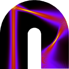
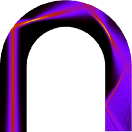
Figure 13: Scattering of an incoming ray of Gaussian shape with unit probability flux at wavenumber $k$, which supports 100 open modes, and for two inner radii $q$ = 0.2, 0.6 (left, right).

We are discussing the scattering over the bend at some fixed wavenumber $k$ and inner radius $q$. The scattering properties are contained in the transmission matrix $T$ (86) and the reflection matrix $R$ (87). The wavefunction over the asymptotic region is described in $N$ modes, where $N\geq N_{\rm o}=\lfloor ka/\pi\rfloor$. We consider an incoming wave coming to the bend from the left side written in the asymptotic region as

$$\psi_{\rm in}({\bf r})=\sum_{n=1}^{N}a_{n}e_{n}^{+}({\bf r})\>.$$ (101)

By introducing a vector of complex coefficients $a=\{a_{n}\}_{n=1}^{N_{\rm o}}$ we can write the transmitted and reflected probability flux, $j_{\rm T}$ and $j_{\rm R}$ respectively, in an elegant form

$$j_{\rm R}=a^{\dagger}\Pi a\>,\qquad j_{\rm T}=a^{\dagger}\Sigma a\>,\qquad j_{0}=a^{\dagger}a=j_{\rm R}+j_{\rm T}\>,$$ (102)

where we introduce matrices $\Pi$ and $\Sigma$ calculated from open-open mode blocks of $R$ and $T$:

$$\Pi=R_{\rm oo}^{\dagger}R_{\rm oo}\>,\quad\Sigma=T_{\rm oo}^{\dagger}T_{\rm oo}\>,\;\textrm{ where }\;\Pi+\Sigma={\rm id}\>.$$ (103)

The average transport properties are given by the first and the second moment of the probability currents $j_{\rm R,T}$ averaged over an ensemble of incoming states $a$. The ensemble represents states (vectors $a$) uniformly distributed over the 2N-dimensional sphere of radius $j_{0}$ [18, 29]. The average probability currents are given by

$${\cal R}=\frac{\left\langle j_{\rm R}\right\rangle_{\alpha}}{j_{0}}=\frac{1}{N_{\rm o}}\operatorname{tr}\{\Pi\}\>,\qquad{\cal T}=1-{\cal R}\>,$$ (104)

and the standard deviations of probability currents (giving fluctuations within an ensemble) are written as

$$\sigma^{2}_{\rm R}=\frac{\left\langle(j_{\rm R}-\left\langle j_{\rm R}\right\rangle_{\alpha})^{2}\right\rangle_{\alpha}}{j_{0}^{2}}=\frac{1}{N_{\rm o}+1}\left[\frac{\operatorname{tr}\{\Pi^{2}\}}{N_{\rm o}}-{\cal R}^{2}\right]=\sigma^{2}_{\rm T}\>.$$ (105)

In the following we thus discuss the average reflection $\cal R$ and the dispersion of reflection $\sigma^{2}_{\rm R}$. An approximation of the transmission matrix $T$ can be determined from the semi-classical calculations, whereas for the reflection matrix $R$ it can not, as the reflection in the bend is a purely quantum phenomenon. The gross structure of matrices $R$ and $T$, similarly as of matrices $A$ and $B$, does not change significantly with increasing wavenumber $k$. In figure 14 we show the density plot of matrices $R$ and $T$ with $N_{\rm o}=100$ open modes. The high probabilities in the matrix $T$ have a classical correspondence, which is revealed through the calculation of the classical scattering matrix $T_{\rm class}$ [30]. Both, the classical and the quantum transmission matrices feature similar patterns, but due to the quantum interference, we can not establish a clear correspondence. In the matrix $T$ we have a large area of high values so we can expect that transmission probability of individual modes should be high. It is important to notice the area in the reflection matrix of high intensity is concentrated around the last open mode with the index $N_{\rm o}$.

$R_{N}$                                      $T_{N}$                                           $T_{\rm class}$

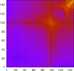
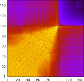
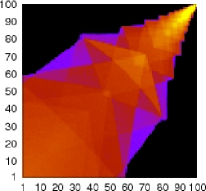
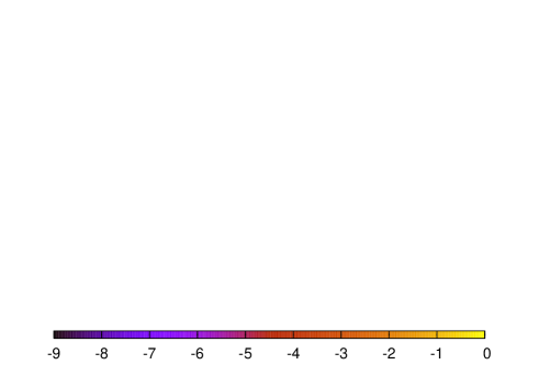
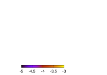
Figure 14: The density plot of the scattering matrices $\log_{10}|(R_{N})_{nm}|$ and $\log_{10}|(T_{N})_{nm}|$ and the classical analog of the later $\log_{10}|(T_{\rm class})_{nm}|$ calculated at inner radius $q=0.6$, wavenumber $k=100.5\frac{\pi}{a}$ and with the total number of modes $N=150$.

At the so called resonant wavenumbers $k_{m}=\frac{\pi}{a}m$ ($m\in{\mathbb{N}}$) a new open mode appears in the asymptotic region and causes a strong increase in the reflection matrix elements at open modes with high indices. This is demonstrated in figure 15, where we show the scattering matrices $R$ and $T$ around the highest open mode calculated calculated at $k\approx k_{100}$ and at $q=0.6$. The changes are centred around the index $N_{\rm o}$ and significantly influence the average transport.

before                        middle                        after

$R_{N}:$

  

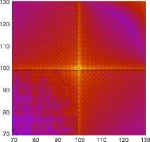
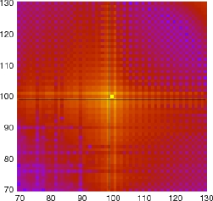
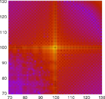
$T_{N}:$

  

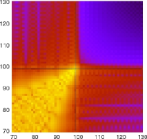
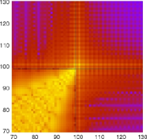
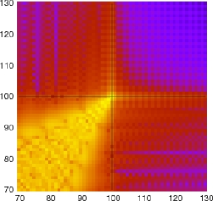
Figure 15: The density plots of the reflection matrix $\log_{10}|(R_{N})_{nm}|$ and the transmission matrix $\log_{10}|(T_{N})_{nm}|$ around the point $(n,m)=(N_{\rm o},N_{\rm o})$ at wavenumbers $k=(100-10^{-3})\frac{a}{\pi}$ (before), $k\doteq 100\frac{a}{\pi}$ (in the middle) and $k=(100+10^{-3})\frac{a}{\pi}$ (after the resonance). The solid lines denote indices $n=N_{\rm o}$ and $m=N_{\rm o}$.

In order to clarify the contributions to the total reflection we plot in figure 16 the reflection probability of individual modes $\Pi_{nn}$ for wavenumbers near and far from the resonance. We see that the highest open mode has the strongest reflection and the reflection probability of “all” modes increases at resonant wavenumbers $k=k_{N_{\rm o}}$. In particular the reflection of highest open mode is almost perfect $\Pi_{N_{\rm o},N_{\rm o}}\approx 1$. In the vicinity of the resonance we could effectively approximate the average reflection as ${\cal R}\approx\Pi_{N_{\rm o},N_{\rm o}}/N_{\rm o}$ (see figure 17).

Figure 16: The diagonal matrix elements $\Pi_{nn}$ at wave-numbers $k=r\frac{\pi}{a}$ as indicated in the figure, and fixed inner radius $q=0.6$. Note that $N_{\rm o}=\lfloor r\rfloor$.

The resonant wavenumbers $k_{N_{\rm o}}$ are important markers for anomalously strong reflection. This is illustrated in figure 17, where we plot the average reflection $\cal R$ as a function of the wave-number around $k=k_{100}$. We see the average reflection $\cal R$ has a strong sharp maximum at resonant wavenumbers and decreases in an irregular oscillating manner with increasing wavenumber until crossing the next resonant wavenumber. The frequency of irregular oscillations increases with increasing wavenumber. From numerical results we see that $\cal R$ decreases with increasing $q$. In narrow channels $a\to 0$ at large wave-numbers we showed with a perturbative approach (see D) that

$${\cal R}\sim\frac{a^{2}}{N_{\rm o}}\>,$$ (106)

which is confirmed numerically. The resonant behaviour around the resonant wavenumber can be partially explained by neglecting all open modes expect the one with the highest index $N_{\rm o}$. Such system can be treated as an independent 1d scatterer ($d=1$) with the reflection and transmission matrix elements reading

$$R_{\rm 1d}=-\frac{\sin(\beta\nu_{N_{\rm o}})}{\sin(\beta\nu_{N_{\rm o}}+{\rm i}\mu_{N_{\rm o}})}\>,\quad T_{\rm 1d}=\frac{\sin({\rm i}\mu_{N_{\rm o}})}{\sin(\beta\nu_{N_{\rm o}}+{\rm i}\mu_{N_{\rm o}})}\>,$$ (107)

with the phase shift

$$\mu_{N_{\rm o}}=2\operatorname{arctanh}\left(K_{N_{\rm o}}\right)\>,\quad K_{p}=\frac{g_{p}A_{p,p}}{\nu_{p}B_{p,p}}\in[0,1]\>.$$ (108)

At $k=k_{N_{\rm o}}$, the mode number $g_{N_{\rm o}}\sim\mu_{N_{\rm o}}$ and the phase shift $\mu_{N_{\rm o}}$ become zero yielding a perfect reflection in a 1d scattering model, $R_{\rm 1d}=-1$ and $T_{\rm 1d}=0$. This treatment is meaningful, because the matrices $A$ and $B$ are approximately diagonal at $(N_{\rm o},N_{\rm o})$ with an algebraic decay of matrix elements when we move away from the diagonal. If the modes were strictly independent we would have $\Pi_{N_{\rm o},N_{\rm o}}=\|R_{\rm 1d}\|^{2}$, but the algebraic tails in matrices $A$ and $B$ make this solution to hold only as a rough approximation as can be seen in figure 17.

(a) (b)

Figure 17: Reflection a bend of an angle $\beta=\pi$ as a function of the wavenumber $k$ in the region of a reflection resonance $k=101\frac{\pi}{a}$. In (a) we show the average reflection measure for different values of $q$ (indicated in the figure), while in (b) we show a zoom-in around the resonance and compare the average reflection and its standard deviation with the reflection in the last open mode (inset shows even a more very narrow region of the resonance).

In figure 18 we study measures of reflection $\cal R$ and $\sigma_{\rm R}$ over a larger range of wave-numbers $k$. From figure 18.a we see that $\cal R$ strongly oscillates with peaks at resonant wave-number $k_{n}$ and its upper bound decreases proportionally to $k^{-1}$, as predicted. The numerical results in figure 18.b indicate that $\sigma_{\rm R}<{\cal R}$ and ${\cal R}\sim\sigma_{\rm R}$ as $k$ goes to infinity.

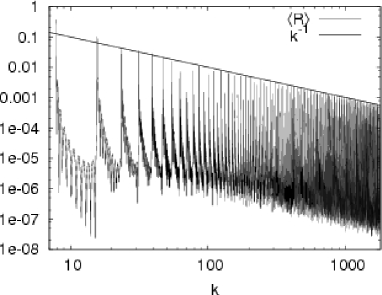
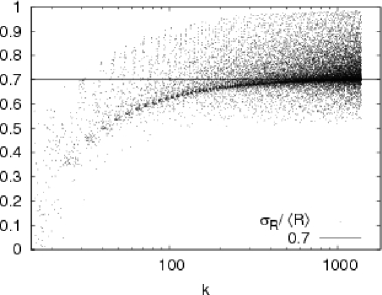
Figure 18: The average reflection $\cal R$ and the relative deviation of reflection $\sigma_{\rm R}$ over a larger interval of wave-numbers $k$ at $q=0.6$.

To get rid of oscillations and get an overall average behaviour of $\cal R$ and $\sigma_{\rm R}$ we calculate their cumulative integrals with respect to the wave-number. The results are shown in figure 19 and yield the following dependence

$$\int_{k_{0}}^{k}{\cal R}\,{\rm d}\kappa\propto\int_{k_{0}}^{k}\sigma_{\rm R}\,{\rm d}\kappa=O(\log(k))\>.$$ (109)

This indicates together with previous conclusions that the reflection measures, averaged over small wave-number ranges, indeed scale as

$${\cal R}\sim\sigma_{\rm R}=O(k^{-1})\>,\quad k\to\infty\>.$$ (110)

It seems that this relation (110) is valid for an arbitrary inner radius $q$ and represents a new and very useful information for the study of wave-guides and general billiards that include bends.

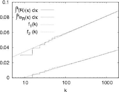
Figure 19: The integral of the average reflection $\cal R$ and deviation $\sigma_{\rm R}$ over larger interval of wave-numbers $k$ of a bend with a radius $q=0.6$ and an angle $\beta=\pi$. The inserted lines are $f_{1}(k)=0.01103+0.01022\log k$ and $f_{2}(k)=-0.01553+0.006924\log k$.

Another insight into the scattering properties gives the Wigner-Smith delay time $\tau_{\rm ws}$ [31, 32], which is the quantum analog of the geometric length travelled by a wave. In the semi-classical limit, where we could apply geometric optics, $\tau_{\rm ws}$ is equal to the average geometric length of classical trajectories over the open billiard. By using the hermitian variant of the lifetime matrix

$$Q=S_{\rm oo}^{\dagger}\frac{{\rm d}S_{\rm oo}}{{\rm d}{\rm i}k}\>,$$ (111)

the Wigner-Smith delay time is defined as

$$\tau_{\rm ws}=\frac{1}{2N_{\rm o}}\operatorname{tr}\{Q\}=\frac{1}{N_{\rm o}}\operatorname{tr}\left\{R_{\rm oo}^{\dagger}\frac{{\rm d}R_{\rm oo}}{{\rm d}{\rm i}k}\right\}+\frac{1}{N_{\rm o}}\operatorname{tr}\left\{T_{\rm oo}^{\dagger}\frac{{\rm d}T_{\rm oo}}{{\rm d}{\rm i}k}\right\}\>,$$ (112)

where we have used block symmetries of our matrix $S$ (73). $\tau_{\rm ws}$ can be thought of as an average delay time corresponding to particular modes, which are defined as

$$\tau^{n}_{\rm ws}=\frac{1}{N_{\rm o}}\sum_{m=1}^{N_{\rm o}}\Im\left\{\left[R_{\rm oo}^{\dagger}\right]_{nm}\left[R_{\rm oo}^{\prime}\right]_{mn}+\left[T_{\rm oo}^{\dagger}\right]_{nm}\left[T_{\rm oo}^{\prime}\right]_{mn}\right\}\>,$$ (113)

with derivative defined as $(\bullet)^{\prime}={\rm d}/{\rm d}k$. Numerical results shown in figure 20 point to a similar dependence of Wigner-Smith delay time $\tau_{\rm ws}$ on the wave-number $k$ as the average reflection $\cal R$, just the oscillations are smoothed out. The time $\tau_{\rm ws}$ strongly increases near the resonance wave-number $k=k_{N_{\rm o}}$ due to intense changes in the scattering matrices $R$ and $T$ in the area around the index of the newly open mode. Qualitatively we can explain the singular behaviour by treating the highest open mode in the resonance regions within 1d scattering model in which the delay time is given by

$$\tau^{\rm 1d}_{\rm ws}=\Im\left\{T_{\rm 1d}^{*}T_{\rm 1d}^{\prime}+R^{*}_{\rm 1d}R_{\rm 1d}^{\prime}\right\}=\frac{\beta\sinh(2\mu_{N_{\rm o}})\nu_{N_{\rm o}}^{\prime}-\sin(2\beta\nu_{N_{\rm o}})\mu_{N_{\rm o}}^{\prime}}{\cosh(2\mu_{N_{\rm o}})-\cos(2\beta\nu_{N_{\rm o}})}\>.$$ (114)

The first term in the numerator of equation (114) corresponds to the transmission and the second term to the reflection. By slowly increasing the wavenumber across the region of the resonance we can notice three different regimes: before, in the vicinity and after the resonant wave-number. Slightly before the resonance $k<k_{N_{\rm o}}$, a new real mode appears in the bend (see formula (121)) making the propagation across the bend very slow. From the formula (114) we learn that this results in a large transmission time and consequently in a large time delay $\tau^{\rm 1d}_{\rm ws}$. In the instance of crossing the reflection resonance a new mode appears in the straight wave-guide, which causes a square-root singularity $\tau^{\rm 1d}_{\rm ws}\sim(k-k_{N_{\rm o}})^{-{1\over 2}}$ for $k>k_{N_{\rm o}}$ and its sign is determined by $2\beta\nu_{N_{\rm o}}$. This reflection term has a short-scale influence to the behaviour of the time delay and can enhance or reduce its size. Obviously, this is a very non-classical situation. By going further away from the resonance wave-numbers the reflection contribution to the time delay is levelled by an increasing transmission term due to a very slow propagation of the mode in the asymptotic region, which again increases the transition time. So we can experience one or two peaks of the time delay in the vicinity of the reflection resonance. Away from the reflection resonance the time delay drops even below the classical time. The latter we assume is due to reflection phenomena which reduces the classically expected phase shift. The presented 1d scattering model has only an instructive purpose and does not represent any useful quantitative approximation, similarly as was the case in the discussion of the reflection.

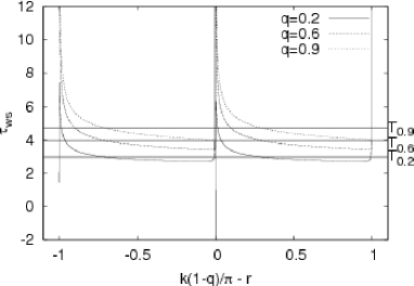
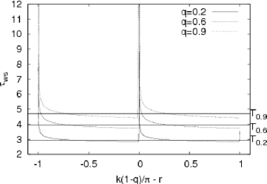
Figure 20: The Wigner-Smith delay time $\tau_{\rm ws}$ for the bend of angle $\beta=\pi$ around the reflection resonance at $r$ = 11, 101 (left,right). The solid horizontal lines with the labels $T_{0.2,0.6,0.9}$ represent the classical delay times at $q=0.2,0.6,0.9$, which are approximately given with the formula $T_{q}=2.45863+2.48696q$.

4 Conclusions

We present mathematical, numerical and physical background of the non-relativistic 2D scattering of a quantum particle on a circular bend connected to infinite straight waveguides. We discuss mathematical properties and derive numerical recipes for accurate and reliable calculation of the mode functions and the corresponding mode numbers in a bend. We take a special care of closed (evanescent) modes in the bend. The obtained modal structure and its properties are incorporated in a robust and stable numerical scheme for computing the scattering matrix with a controllable precision. Our numerical apparatus is applied to the study of transport properties. We focus mainly on the reflection, which is a purely quantum (wave) phenomenon since the back-reflection of classical rays is not possible. Our study is particularly focused on the possibility to investigate the (semi-classical) regime of very large wave-numbers. Some of the obtained physical properties of the scattering problem can be explained analytically. In addition, we present results on the Wigner-Smith delay in the bend. The obtained transport properties can be useful in discussing and predicting properties of open billiards (or wave guides) composed of arbitrary combination of bends and straight segments.

References

Appendix A The symmetry of mode numbers

We prove the symmetry (15), by changing the variable $r=e^{-x}$ and transforming the Bessel equation (3) and the corresponding boundary condition into the equation

$$\frac{{\rm d}^{2}Z}{{\rm d}x^{2}}+\left(k^{2}e^{-2x}-\nu^{2}\right)Z=0\>,\qquad Z|_{x=0,\log q}=0\>,$$ (115)

which can be interpreted as a one-dimensional quantum mechanical eigenvalue problem, with the Hamiltonian $\hat{H}$ and potential $V^{\prime}$:

$$\hat{H}Z=-\nu^{2}Z\>,\quad\hat{H}=-\frac{{\rm d}^{2}}{{\rm d}x^{2}}+V^{\prime}(x)\>,\quad V^{\prime}(x)=\left\{\begin{array}[]{lll}-k^{2}e^{-2x}&:&x\in[0,-\log q]\cr\infty&:&\textrm{elsewhere}\end{array}\right.\>.$$ (116)

Because the Hamiltonian $\hat{H}$ is a Hermitian operator, the eigenvalues are real $-\nu^{2}\in{\mathbb{R}}$ yielding $\nu\in{\mathbb{R}}\cup{\rm i}{\mathbb{R}}$. From the form of the potential $V^{\prime}(x)$, depicted in figure 21, we see that there are only finite number of real mode numbers $\nu^{2}>0$ and infinite number of imaginary mode numbers $\nu^{2}<0$. The independent solution of equation (116) are orthogonal with respect to the measure ${\rm d}x=r^{-1}\,{\rm d}r$ and so the weight function between mode functions $U_{p}(r)$ in the bend is $w(r)=r^{-1}$.

Figure 21: The analog of the quantum potential in the eigenvalue equation for the mode functions in the bend.

Appendix B The number of modes in the straight and the bent waveguide

We discuss the number of open modes $N_{\rm b}(k,q)=\operatorname{card}\Re\{{\cal M}_{k,q,+}\}$ in the bend and its deviation from the number of modes in the straight waveguide $N_{\rm s}=\lfloor ka/\pi\rfloor$. The mode numbers in ${\cal M}_{k,q,+}$ continuously slide with increasing $k$ and fixed $q$ from the imaginary to the real axis by crossing the point $\nu=0$. This dynamics is depicted in figure 2. This means that $N_{\rm b}(k,q)$ is equal to the number of zeros $x$ of $Z_{0,x}(q)$ up to the value $k$

$$N_{\rm b}(k,q)=\operatorname{card}\Re\{{\cal M}_{k,q,+}\}=\operatorname{card}\{x\leq k:Z_{0,x}(q)=0\}\>.$$ (117)

By using substitutions $U=r^{-{1\over 2}}\varphi$ and $r=q+ax$ the mode problem in the bend (5) is in the case $\nu=0$ transformed into a 1d stationary Schrödinger equation $(\gamma=q/(1-q))$

$$-\frac{{\rm d}^{2}\varphi}{{\rm d}x^{2}}+V(x)\varphi=e\varphi\>,\quad V(x)=-[2(x+\gamma)]^{-2}\>,\quad x\in[0,1]\>,$$ (118)

with the eigen-energy dentoed by $e=(ka)^{2}$. The discrete set of eigen-energies is ordered as $e_{n+1}>e_{n}$, $n\in{\mathbb{N}}$. By setting $V=0$ in expression (118) we obtain the mode problem for appropriately rescaled straight waveguide. In the eigen-energies in this case se $(\pi n)^{2}$, $n\in{\mathbb{N}}$. Then taking into account the (empirical) fact $e_{n}\leq(\pi n)^{2}<e_{n+1}$ we can conclude

$$0\leq N_{\rm b}(k,q)-N_{\rm s}(k,q)\leq 1\>,\qquad\forall q\in(0,1)\>.$$ (119)

This means that at certain $k$ and $q$ we can have in the bend one open mode more, but not less than in the straight waveguide. In the semi-classical limit $k\to\infty$ the eigen-energies $e_{n}$ can be obtained using the Debye approximation valid for $qk\gg 1$. In this way we get a relation between the eigenvalues $e$ and its counting number $N_{\rm b}$

$$2\pi N_{\rm b} = \left(4k^{2}+1\right)^{1\over 2}-\left(4(qk)^{2}+1\right)^{1\over 2}$$ (120)

$$- \operatorname{arctan}\left((4k^{2}+1)^{-{1\over 2}}\right)+\operatorname{arctan}\left((4(qk)^{2}+1)^{-{1\over 2}}\right)\>,$$

which yields with asymptotic expansion in $k$ the expression

$$N_{\rm b}(k,q)=\frac{ka}{\pi}+\frac{a}{8\pi kq}+\frac{a(1+q)}{64\pi(qk)^{2}}+O\left(a(qk)^{-3}\right)\>.$$ (121)

We see that $N_{\rm b}$ and $N_{\rm s}$ are close to each other for high wave-number and and not too small inner radius $q$.

Appendix C The method of concatenating scattering matrices

Here we outline a method to concatenate the scattering matrices [33] associated to scatterers on sectioned wave guides. Let us assume to have two scatterers labelled by A and B and with scattering matrices $S_{\rm A}$ and $S_{\rm B}$, respectively.

$$S_{\rm A,B}={\left[\begin{array}[]{cc}r_{\rm A,B}^{\rm L}&t_{\rm A,B}^{\rm R}\cr t_{\rm A,B}^{\rm L}&r_{\rm A,B}^{\rm R}\end{array}\right]}\in{\mathbb{C}}^{2N\times 2N}\>.$$ (122)

By combining both scatterers A and B in the order AB we build a “larger” scatterer with the scattering matrix $S$. The matrix $S$ is calculated from matrices $S_{\rm A,B}$ by a nonlinear operation $\odot:{\mathbb{C}}^{2N\times 2N}\times{\mathbb{C}}^{2N\times 2N}\to{\mathbb{C}}^{2N\times 2N}$ defined as

$$S=S_{\rm A}\odot S_{\rm B}={\left[\begin{array}[]{cc}r^{\rm L}&t^{\rm R}\cr t^{\rm L}&r^{\rm R}\end{array}\right]}\in{\mathbb{C}}^{2N\times 2N}\>,$$ (123)

which explicitly reads

$$r^{\rm L}=r_{\rm A}^{\rm L}+t_{\rm A}^{\rm R}r_{\rm B}^{\rm L}L^{-1}t_{\rm A}^{\rm L}\>,\quad t^{\rm L}=t_{\rm B}^{\rm L}L^{-1}t_{\rm A}^{\rm L}\>,$$ (124)

$$r^{\rm R}=r_{\rm A}^{\rm R}+t_{\rm A}^{\rm L}r_{\rm B}^{\rm R}{L^{\prime}}^{-1}t_{\rm A}^{\rm R}\>,\quad t^{\rm R}=t_{\rm B}^{\rm R}{L^{\prime}}^{-1}t_{\rm A}^{\rm R}\>,$$ (125)

where we define $L=1-r_{\rm A}^{\rm R}r_{\rm B}^{\rm L}$ and $L^{\prime}=1-r_{\rm B}^{\rm L}r_{\rm A}^{\rm R}$. Note that a bend on a straight waveguide can be treated as a scatterer. By combining bends of angles $\gamma^{\prime}$ and $\delta^{\prime}$ with scattering matrices $S(\gamma^{\prime})$ and $S(\delta^{\prime})$, respectively, we get a bend of angle $\gamma^{\prime}+\delta^{\prime}$ with the scattering matrix $S(\gamma^{\prime}+\delta^{\prime})$. The latter matrix can be obtained from matrices $S(\gamma^{\prime})$ and $S(\delta^{\prime})$ by the formula

$$S(\gamma^{\prime}+\delta^{\prime})=S(\gamma^{\prime})\odot S(\delta^{\prime})=S(\delta^{\prime})\odot S(\gamma^{\prime})\>.$$ (126)

Appendix D Perturbative calculation of the scattering matrix for narrow bent wave-guide

We present a semi-classical approximation, for $k\gg 1$, of a scattering matrix corresponding to a single bend on a straight wave-guide of width $a$, as one shown in figure 1. Here we are discussing only narrow channels $a\ll 1$, where the influence of closed modes on the scattering diminishes. Therefore closed modes are neglected in our calculations. We are working at wavenumbers $k$, where in all regions of the open-billiard the number of open modes is equal. This enables us to write the reflection and the transmission matrix in the following simpler form

$$R=-[C_{+}-{\rm i}S_{+}]^{-1}(C_{-}+{\rm i}S_{-})\>,\qquad T=2[C_{+}-{\rm i}S_{+}]^{-1}\>,$$ (127)

where we use the diagonal matrices ${\cal C}=\Re\{{\cal F}\}$, ${\cal S}=\Im\{{\cal F}\}$ and $G=\operatorname{diag}\{g_{n}\}_{n=1}^{N_{\rm o}}$ to express the introduced matrices

$$C_{\pm} = G^{1\over 2}A{\cal C}B^{T}G^{-{1\over 2}}\pm G^{-{1\over 2}}B{\cal C}A^{T}G^{1\over 2}\>,$$ (128)

$$S_{\pm} = G^{1\over 2}A{\cal S}A^{T}G^{1\over 2}\pm G^{-{1\over 2}}B{\cal S}B^{T}G^{-{1\over 2}}\>.$$ (129)

We proceed by rescaling the variables to dimensionless form by the following substitutions

$$\hskip 28.45274pty=a\xi\>,\quad r=q+a\xi\>,\quad\kappa=ak\>,\quad h_{n}=ag_{n}=\sqrt{\kappa^{2}-(\pi n)^{2}}\>,\quad\nu_{p}=\alpha v_{p}\>,$$ (130)

with a new transverse coordinate $\xi\in[0,1]$, and geometric properties being described by the parameter $\alpha=a/q\ll 1$. The transition matrices are then expressed as

$$A_{np}=q^{1\over 2}Q_{np}\>,\quad Q_{np}=\frac{\int_{0}^{1}{\rm d}\xi\;b_{n}(\xi)\phi_{p}(\xi)(1+\alpha\xi)^{-{1\over 2}}}{\sqrt{\int_{0}^{1}\phi_{p}(\xi)^{2}(1+\alpha\xi)^{-2}}}\>,$$ (131)

$$B_{np}=q^{-{1\over 2}}P_{np}\>,\quad P_{np}=\frac{\int_{0}^{1}{\rm d}\xi\;b_{n}(\xi)\phi_{p}(\xi)(1+\alpha\xi)^{-{3\over 2}}}{\sqrt{\int_{0}^{1}\phi_{p}(\xi)^{2}(1+\alpha\xi)^{-2}}}\>.$$ (132)

with $b_{n}(\xi)=\sqrt{2}\sin(\pi n\xi)$. The eigen-pairs $(v_{p},\phi_{p}(\xi))$ are defined by the following differential equation and the boundary condition:

$$\frac{{\rm d}^{2}\phi_{p}}{{\rm d}\xi^{2}}+\left(\kappa^{2}-\frac{v_{p}^{2}-\frac{\alpha^{2}}{4}}{(1+\alpha\xi)^{2}}\right)\phi_{p}=0\>,\qquad\phi_{p}(0)=\phi_{p}(1)=0\>.$$ (133)

We can easily recognize that the solutions of equation (133) converge in the limit $\alpha\to 0$ to $v_{p}=h_{p}$ and $\phi_{p}(\xi)=b_{p}(\xi)$. We assume that the solutions can be expanded in a power series of variable $\alpha$. The eigen-pairs can then be obtained using the standard perturbation theory with the perturbation parameter $\alpha$. The rescaled mode numbers are written as

$$v_{p}^{2}=h_{p}^{2}\left[1+\alpha+\alpha^{2}\left(\frac{1}{3}-\frac{1}{2(\pi p)^{2}}\right)\right]+\alpha^{2}\left(\frac{1}{4}+O(h_{p}^{4})\right)+O(\alpha^{3})\>,$$ (134)

and the rescaled mode functions read as

$$\phi_{p}(\xi)=\sum_{n}V_{np}\,b_{n}(\xi)\>,\quad V_{np}=\delta_{np}+\alpha\frac{8np\,h_{p}^{2}}{\pi^{4}(n^{2}-p^{2})^{3}}\delta_{n+p}^{\rm odd}+O(\alpha^{2})\>,$$ (135)

where we use the symbol $\delta_{n}^{\rm odd}=(1:n\textrm{ is odd};\;0:\textrm{otherwise})$. By plugging the mode functions $\phi_{p}(\xi)$ (134) into transition matrices $Q$ (131) and $P$ (132) we obtain

$$Q_{np}=\delta_{np}+\alpha\left(F_{np}+\frac{1}{4}\delta_{np}\right)+O(\alpha^{2})\>,$$ (136)

$$P_{np}=\delta_{np}-\alpha\left(F_{pn}+\frac{1}{4}\delta_{np}\right)+O(\alpha^{2})\>,$$ (137)

$$F_{np}=\frac{8np}{\pi^{2}(n^{2}-p^{2})^{2}}\left(\frac{h_{p}^{2}}{\pi^{2}(n^{2}-p^{2})}-\frac{1}{4}\right)\delta_{n+p}^{\rm odd}\>.$$ (138)

Note that the rescaled transition matrices $Q$ and $P$ satisfy the known identity $QP^{T}=PQ^{T}={\rm id}$. We insert the expressions for $Q$ (136) and $P$ (137) back into $S_{\pm}$ (129) and $C_{\pm}$ (128) and write the reflection and the transmission matrix as

$$R=-\frac{\alpha}{2}{\cal F}\left[H^{\frac{1}{2}}\left([F,{\cal C}]+{\rm i}(F{\cal S})^{\rm s}\right)H^{-\frac{1}{2}}+H^{-\frac{1}{2}}\left([F^{T},{\cal C}]+{\rm i}(F^{T}{\cal S})^{\rm s}\right)H^{\frac{1}{2}}\right]+O(\alpha^{2})\>,$$ (139)

$$T={\cal F}-\frac{\alpha}{2}\left(H^{\frac{1}{2}}[{\cal F},F]H^{-\frac{1}{2}}+H^{-\frac{1}{2}}[F,{\cal F}]H^{\frac{1}{2}}\right)+O(\alpha^{2})\>.$$ (140)

where we have introduced the symbol $(A)^{\rm s}=A+A^{T}$ and the diagonal matrix $H=\operatorname{diag}\{h_{n}\}_{n=1}^{N_{\rm o}}$. The approximations of the reflection matrix $R$ (139) and the transmission matrix $T$ (140) are valid far away from the resonant condition $ak=\pi n$, because we assumed that $|g_{m}|>\alpha$ for all $m\leq N_{\rm o}$. We conclude that the strength of reflection scales as ${\cal R}\sim\alpha^{2}$ and that narrow channels can be treated as perturbed straight wave-guides.

References

- [1] Strutt J W 1897 On the passage of electric waves through tubes or the vibrations of dielectric cylinders Phil. Mag. (Ser. 5) 53 125–132
- [2] Jensen H and Koppe H 1971 Quantum mechanics with constraints Ann. Phys. 63 586–91
- [3] Exner P and Seba P 1989 Bound states in curved quantum waveguides J. Math. Phys. 30 2574–80
- [4] Exner P 1993 Bound states in quantum waveguides of slowly decaying curvature J. Math. Phys. 34 23–28
- [5] Lin K and Jaffe R L 1996 Bound states and threshold resonances in quantum wires with circular bends Phys. Rev. B 54 5750–62
- [6] Londergan J T and Carini J Pand Murdock D P 1999 Binding and scattering in two-dimensional systems: application to quantum wires, waveguides and photonic crystals, Lecture Notes in Physics, volume 60 (Berlin [etc]: Springer Verlag)
- [7] Spivack M, Ogilvy J and Sillence C 2002 Electromagnetic propagation in the curved two-dimensional waveguide Waves Random Media 12 47–62
- [8] Lent C S 1990 Transmission through a bend in an electron waveguide Appl. Phys. Lett. 56 2554–6
- [9] Cochran J A and Pecina R G 1966 Mode propagation in continuously curved waveguides Radio science 1 679–96
- [10] Accation L and Bertin G 1990 Modal analysis of curved waveguides in Proc.20th Eur, Microwave Conf. Budapest sep. 1990
- [11] Sols F and Macucci M 1990 Circular bends in electron waveguides Phys. Rev. B 41 11887–91
- [12] Sprung D W L and Wu H 1992 Understanding quantum wires with circular bends J. Appl. Phys. 71 515–7
- [13] Rashid M A and Kodama M 2002 Analysis of propagation properties in junctions between straight and bend waveguides using cylindrical functions of complex orders in Proc. ITC-CSCC-2002 Conference July, 2002, Phuket, Thailand
- [14] Amari S and Bornemannm J 2000 Modelling of propagation and scattering in waveguide bends in Proc. 30th European Microwave Conf. Paris, France, Oct. 2000 Vol. 2 353–6
- [15] Cochran J A 1964 Remarks on the zeros of cross-product Bessel functions J. Soc. Indust. Appl. Math. 12 580–7
- [16] Cochran J A 1966 The analyticity of cross-product Bessel function zeros Proc. Camb. Phil. Soc 62 215–56
- [17] Cochran J A 1966 The asymptotic nature of zeros of cross-product Bessel function Quart. Journ. Mech. and Applied Math. 19 511–22
- [18] Newton R G 2002 Scattering Theory of Waves and Particles (Mineola, New York: Dover Publications, inc.)
- [19] Olver F W J 1972 Bessel functions of integer order in Handbook of Mathematical Functions 10th ed., eds. Abramowitz M and Stegun I A (New York: Dover) pp 355–389
- [20] Olver F W J 1962 Tables for Bessel functions of moderate or large orders in Mathematical Tables vol. 6 (Her Majesty’s Stationary office, London, England)
- [21] Morse P M and Feshbach H 1953 Methods of Theoretical physics, vol. 1 (New York: McGraw Hill)
- [22] Fong K W, Jefferson T H, Suyehiro T and Walton L 1993 SLATEC common mathematical library, version 4.1
- [23] Erdélyi A 1955 Higher transcendental functions, vol. II (New York, Toronto, London: McGraw-Hill)
- [24] Luke Y L 1962 Integrals of Bessel functions (New York, Toronto, London: McGraw-Hill, cop.)
- [25] Demmel J W 1997 Applied numerical linear algebra (SIAM)
- [26] Prosen T 1995 General quantum surface-of-section method J. Phys. A: Math. Gen 28 4133–55
- [27] Bogomolny E B 1992 Semiclassical quantization of multidimensional systems Nonlinarity 5 805–66
- [28] Horvat M and Prosen T 2004 Uni-directional transport properties of a serpent billiard J. Phys. A: Math. Gen 37 3133–3145 (Preprint nlin.CD/0601055)
- [29] Prosen T and Žnidarič M 2002 Stability of quantum motion and correlation decay J. Phys. A: Math. Gen. 35 1455–81
- [30] Méndez-Bermudéz J A e a 2002 Understanding quantum scattering properties in terms of purely classical dynamics: Two-dimensional open chaotic billiards Phys. Rev. E 66 046207
- [31] Wigner W P 1955 Lower limit for the energy derivative of the scattering phase shift Phys. Rev. 98 145–7
- [32] Smith F T 1960 Lifetime matrix and the collision theory Phys. Rev. 118 349–56
- [33] Mayer A and Vigneron J P 1999 Accuracy-control techniques applied to stable transfer-matrix computations Phys. Rev. E 59 4659–65